Activation of Shaker Potassium Channels

Abstract

The conformational changes associated with activation gating in Shaker potassium channels are functionally characterized in patch-clamp recordings made from Xenopus laevis oocytes expressing Shaker channels with fast inactivation removed. Estimates of the forward and backward rates for transitions are obtained by fitting exponentials to macroscopic ionic and gating current relaxations at voltage extremes, where we assume that transitions are unidirectional. The assignment of different rates is facilitated by using voltage protocols that incorporate prepulses to preload channels into different distributions of states, yielding test currents that reflect different subsets of transitions. These data yield direct estimates of the rate constants and partial charges associated with three forward and three backward transitions, as well as estimates of the partial charges associated with other transitions. The partial charges correspond to an average charge movement of 0.5 e₀ during each transition in the activation process. This value implies that activation gating involves a large number of transitions to account for the total gating charge displacement of 13 e₀. The characterization of the gating transitions here forms the basis for constraining a detailed gating model to be described in a subsequent paper of this series.

introduction

Voltage-gated sodium, calcium, and potassium channels underlie the electrical properties of excitable cells. Insights into the structural changes involved in the voltage-dependent opening of these channels first came from functional studies performed in the squid axon (Hodgkin and Huxley, 1952a , 1952b ). The steep voltage sensitivity of the observed potassium and sodium conductances suggested that the channel opening process involves the displacement of a large amount of charge across the cell membrane. The long delay in the time courses of activation implied that channel opening involves multiple kinetic steps. The structural origins of these functional properties are now becoming clear. The alpha subunits of voltage-gated sodium and calcium channels are each encoded by a single long transcript with four homologous regions (Noda et al., 1984; Tanabe et al., 1987), while voltage-gated potassium channels are encoded by a transcript that is approximately one-fourth as long (Tempel et al., 1987; Kamb et al., 1988), with a channel complex formed by four subunits (MacKinnon, 1991; Kavanaugh et al., 1992; Li et al., 1994). A requirement for separate activation of each of these units helps to explain the delay in channel activation. Each of the protomers or subunits of these channels contains a putative transmembrane segment S4 that has a number of conserved basic residues and is a candidate for the charged region of the channel that moves in response to voltage, leading to channel activation (Guy and Seetharamulu, 1986; Noda et al., 1986). Mutations in the S4 region yield large effects on the voltage dependence of activation (Stühmer et al., 1989; Liman et al., 1991; Lopez et al., 1991; McCormack et al., 1991; Papazian et al., 1991; Logothetis et al., 1992; summarized in Sigworth, 1994). Also, it has been shown recently that membrane potential changes cause changes in accessibility of S4 residues (Yang and Horn, 1995; Yang et al., 1996; Mannuzzu et al., 1996; Larsson et al., 1996), and that S4 charge changes cause changes in total gating charge movement (Aggarwal and MacKinnon, 1996; Seoh et al., 1996).

Insights into the mechanics of activation gating have also come from extensions of the functional studies that were first performed by Hodgkin and Huxley (1952a , 1952b ). In voltage-clamp measurements of macroscopic and single-channel ionic currents, various voltage protocols have been used to emphasize particular steps in the activation process (Cole and Moore, 1960). The voltage-dependent transitions among closed states have also been characterized from the time courses of gating currents, which are the direct electrical manifestation of the charge displacements associated with conformational changes (Armstrong and Bezanilla, 1973; Schneider and Chandler, 1973; Keynes and Rojas, 1974). Additionally, the fluctuations in the gating currents can provide information about the size of the charge displacements in single gating transitions (Conti and Stühmer, 1989; Crouzy and Sigworth, 1993; Sigg et al., 1994b ). Ultimately, the understanding of voltage gating in ion channels will require combining this detailed functional information with experiments that give more direct structural information.

Examples of the value of detailed functional studies are seen in the recent work on the Shaker potassium channel (Bezanilla et al., 1991; Stühmer et al., 1991; Schoppa et al., 1992; Bezanilla et al., 1994; Hoshi et al., 1994; McCormack et al., 1994; Perozo et al., 1994; Stefani et al., 1994; Zagotta et al., 1994 a, 1994b). Shaker channels have been a favorite in the study of activation gating for a variety of reasons. They can be made noninactivating through a NH₂-terminal truncation (Hoshi et al., 1990) and they express well in Xenopus oocytes, allowing the measurement of gating currents as well as ionic currents. Also, because they are tetramers, the presumed fourfold functional symmetry of Shaker channels can be exploited in developing simpler kinetic models. The major results from the recent studies on these channels may be summarized as follows.

(a) The total gating charge per channel is ∼13 e₀. This value was obtained from calibrated measurements of gating currents (Schoppa et al., 1992; Aggarwal and MacKinnon, 1996; Seoh et al., 1996), and corroborated by measurements of limiting voltage sensitivity (Zagotta et al., 1994 a; Seoh et al., 1996).

(b) Between the resting and the open state, the channel undergoes a minimum of five kinetic transitions, as estimated from the time course of channel opening in response to a voltage step (Zagotta et al., 1994 a).

(c) The time course of the “on” gating current induced by a step depolarization has a rising or plateau phase (Bezanilla et al., 1994), implying that the first kinetic steps in channel activation are slower or less voltage dependent than subsequent steps.

(d) After large depolarizations, the time course of the “off” gating current induced by a voltage step back to the holding potential has a rising phase (Bezanilla et al., 1991) and also decay kinetics that match the time course of channel deactivation (Zagotta et al., 1994 a). Thus, the first kinetic steps in channel deactivation are slower than subsequent steps.

(e) At intermediate voltages, the gating currents display a fast component that is followed by a slow exponential component that is correlated with channel opening (Bezanilla et al., 1994). Also, at these voltages, the ionic currents have a relatively short delay, followed by a very slow rise to the peak current (Zagotta et al., 1994 a). These phenomena imply that channel opening at these voltages is much slower than the rate that the channel traverses through early closed states.

(f) Shaker's voltage dependence of charge movement (Q-V) relation is shallow at hyperpolarized voltages but is steeper over the voltage range where channels open (Stefani et al., 1994; Bezanilla et al., 1994).

(g) Components of charge in the Q-V relation have been shown to be differentially affected by some mutations in the S4 region (Schoppa et al., 1992; Perozo et al., 1994) and also by drug binding (McCormack et al., 1994). The differential effects suggest the existence of different types of voltage-dependent conformational changes.

(h) Measurements of gating current fluctuations suggest that elementary charge movements are roughly 2 e₀ in size (Sigg et al., 1994b ; Sigworth, 1994).

(i) The distribution of channel open times is well described by a single exponential function (Hoshi et al., 1994), which is consistent with Shaker channels having a single open state. The single channel data also suggest the presence of closed states that are not in the main activation path (Hoshi et al., 1994).

Several kinetic models have been proposed that take into account subsets of these functional properties for Shaker channels (Schoppa et al., 1992; Tytgat and Hess, 1992; Bezanilla et al., 1994; McCormack et al., 1994; Zagotta et al., 1994 b). Interestingly, however, these models have little in common with each other, with different models explaining the same functional data through very different mechanisms. For example, the steep voltage dependence of charge movement and channel opening is explained in the model proposed by Bezanilla et al. (1994) by a transition with a large valence, while the model of Zagotta et al. (1994 b) achieves this through smaller charge movements but with a slow channel closing rate. The discrepancies between the models point to the need of further analysis of the activation properties of Shaker channels.

In this paper and the two papers that follow (Schoppa and Sigworth, 1998a , 1998b ), we present further functional studies on activation gating in Shaker potassium channels. Our general strategy is to perform a systematic study of the different gating steps in Shaker's activation process. This first paper will focus on measurements of macroscopic ionic and gating currents measured at extreme depolarizations and hyperpolarizations, which yield estimates of forward and backward rates. Some of the described experiments are similar to those that have been reported previously, but new insights into the activation gating process are gained by analyzing the data in new ways, and also by extending the voltage range of the current measurements. The channel studied, which has its NH₂ terminus truncated to remove fast inactivation, will be referred to as wild type (WT)¹ to distinguish it from a mutant channel (V2) that will be the focus of the second paper. The third paper will use results from both WT and V2 channels to develop a new kinetic model for Shaker channel activation.

methods

Channel Expression

The construction of noninactivating WT Shaker 29-4 cDNAs and in vitro synthesis of cRNA have been described previously (Iverson et al., 1990; Schoppa et al., 1992). Channels were expressed in Xenopus laevis oocytes injected with ∼3 ng cRNA for recordings of macroscopic ionic and gating currents, and 50–100-fold less cRNA for single channel recordings. Current measurements were made 4–21 d after injection with the patch-clamp technique (Hamill et al., 1981) using an EPC-9 patch clamp amplifier (HEKA Electronic, Lambrecht, Germany).

Measurements of Macroscopic Ionic and Gating Currents

Macroscopic ionic and gating currents were recorded in inside-out membrane patches using conventional oocyte macropatch techniques (Stühmer et al., 1991). Patch recordings used pipettes pulled from Kimax capillary tubes with tip diameters ranging from 3 to 10 μm (0.5–3.0 MΩ resistance). Voltage pulses were applied from a holding potential of −93 mV. Current signals were filtered (unless otherwise indicated) at 10 and 5 kHz (Bessel characteristic) for recordings of ionic and gating currents, respectively. Data were sampled at five to seven times the filtering frequency. For subtraction of linear leak and capacitive currents in recordings of macroscopic ionic currents, alternating positive and negative pulses of 20-mV amplitude from a −133-mV leak holding potential were applied, and the resulting current was scaled appropriately. For gating currents, a scaled current response induced by only a negative going voltage pulse from −133 to −153 was subtracted. This modification reduced the artifact in leak subtraction from charge movement at voltages positive to −133 mV (Stühmer et al., 1991). To increase the signal-to-noise ratio, 10–100 sweeps were averaged before the data were stored. The pulse frequency was set to be high (1–5 Hz) to allow rapid measurement of many sweeps, but we determined that the frequencies used did not induce rundown of the ionic or gating currents, arising from slow inactivation. Displayed gating current traces were sometimes additionally filtered with a Gaussian digital filter to 2.5–3.5 kHz.

Most of the ionic current measurements were made with pipettes filled with 140 mM N-methyl-d-glucamine (NMDG) aspartate (Asp), 1.8 mM CaCl₂, and 10 mM HEPES, and the bath solution contained 139 mM KAsp, 1 mM KCl, 1 mM EGTA, and 10 mM HEPES. Most of the gating current measurements were made with the same solutions, except with 2 μM charybdotoxin (CTx) added to the pipette solution to block ionic currents (Lucchesi et al., 1989). CTx did not appear to alter the properties of the charge movement, as the currents recorded in the presence of CTx were similar to those recorded in the absence of CTx but with NMDG⁺ replacing K⁺ in the bath to remove the ionic current. Membrane potential values were corrected for a liquid junction potential at the interface of the NMDG⁺ pipette and K⁺ bath solutions, which we estimated to be −13 mV (Neher, 1992). All experiments were done at room temperature. The bath chamber was not perfused in these experiments.

Voltage steps to very positive and negative voltages were kept short (≤5 ms at V > +100 mV and V < −120 mV) to reduce contamination of the recorded ionic currents by endogenous oocyte currents. Corresponding gating current recordings made in the presence of CTx showed little background current, suggesting that contamination of our ionic currents by endogenous currents is likely to be negligible.

The large pipette sizes used in recordings of gating currents encouraged the formation of membrane vesicles or partial vesicles when the patch was pulled off the oocyte. Gating current recordings were rejected if the measured on current did not show an instantaneous component of the rising phase: specifically, a component with amplitude at least 50% of the peak on current was expected to rise with the same time course as the measured step response of the recording system (see below). Further, recordings with very large ionic currents (>2.5 nA) were rejected to avoid errors due to series resistance.

To allow the interpretation of the rapid gating events reflected in the recordings of ionic tail currents and reactivation time courses, the step response of the recording system, including the filter, was determined by injecting a step of current into the patch clamp head stage using the test facility of the EPC-9 and measuring the current response. At the low gains at which the macroscopic ionic and gating currents were measured (500 MΩ feedback resistor), the response time, defined as the time required for the current to reach 50% of its peak in response to a step current input, was found to be 40 and 25 μs at the 10 and 15 kHz filtering bandwidths used for most ionic current measurements, respectively. Other delays in the stimulus and recording system were expected to be negligible: the stimulus filter risetime was set at 2 μs for measurements of tail currents and reactivation time courses, while the patch membrane charging time constant was expected to be below 1 μs. To account for the total delays, the recorded current traces were offset in time by three sample intervals. In the measured time course of the step response of the recording system, it was also determined that an additional approximately three sample intervals were required for the step response to settle to near its final level. Thus, an additional three sample intervals were always ignored in the fitting of exponentials to the tail current and reactivation time courses.

The time courses of the macroscopic ionic and gating currents were fitted to the sums of exponentials by least squares within the Igor data analysis program (WaveMetrics, Lake Oswego, OR). The derived parameter estimates were consistently independent of the initial guesses supplied.

In the text, errors in all measured quantities are given as the mean ± SEM.

Measurement of Single-Channel Ionic Currents

Single-channel recordings were made in inside-out patches in response to step depolarizations from a −93-mV holding potential. Patch pipettes were pulled from 7052 glass (Garner Glass, Claremont, CA) with 1–2-μm tip diameters (4–10 MΩ resistance). The recording solutions were identical to those used in the measurements of macroscopic ionic currents. Filtering and sampling frequencies were variable, appropriate for the amplitude of the single-channel activity at a given voltage. Leak subtraction was performed by subtracting an average of 8–20 of the nearest null traces. To allow the measurement of a large number of single channel sweeps, the pulse frequency was set to be high (1–5 Hz); however, there was no indication of slow inactivation, which would have caused a time-dependent increase in the number of null traces. The displayed single channel data are filtered at the frequencies used for the event detection, as described below.

The single-channel activity apparently arose from Shaker channels since (a) no such single channel activity was observed in patches in which CTx was included in the pipette, and (b) the ensemble averages of WT's single-channel current traces were kinetically identical to the macroscopic currents in patches from oocytes injected with 50–100-fold more cRNA. Infrequently, a patch would display other single-channel activity, but this activity was easily distinguishable from Shaker's in its voltage-dependence, kinetics, and conductance properties.

The analysis of the equilibrium single-channel closed and open times was performed with the TAC single-channel analysis program, which is based on THAC (Sigworth, 1983). Data were filtered with a digital Gaussian filter to achieve an appropriate signal-to-noise ratio, and event detection was performed using the standard half-amplitude threshold analysis (Colquhoun and Sigworth, 1995). Complicating the analysis of the single-channel events was the presence of apparent subconductance activity (Hoshi et al., 1994). The event detection for a given trace was stopped at the time point at which the channel first exhibited such behavior. Ignoring these data was unlikely to introduce a significant error in our results since subconductance activity was relatively infrequent: in one patch recording of 613 consecutive traces of single channel activity at +27 mV, the open channel spent only 14% of the total 16.6 s of recorded open time at a subconductance level. Here a subconductance level was defined to be an amplitude level smaller than 75% of the most common amplitude level.

For the construction of closed- and open-time histograms, the deadtime (T _d) for a given analysis filtering frequency f _c was taken to be T _d = 0.179/f _c and short-event durations were adjusted appropriately for Gaussian filtering as described (Colquhoun and Sigworth, 1995). Closed and open times were binned logarithmically and the square root of the number of events was plotted (Sigworth and Sine, 1987). The minimum-duration bin for each histogram was set to be the deadtime corresponding to the analysis filtering frequency used for the event detection. The event histograms were fitted to a mixture of exponential components with the amplitudes and time constants adjusted using the binned maximum likelihood method (Sigworth and Sine, 1987). The number of exponential components fitted to the histograms was determined by the likelihood ratio test for nested models (Horn and Lange, 1983), which can be applied to the problem of comparing fits with different numbers of exponentials (McManus and Magleby, 1988).

Accounting for Three Artifacts

In the following section, we describe how we accounted for three additional potential artifacts that could affect our interpretation of the data.

Effects of different recording solutions.

While most of the recordings were made with the bath and pipette solutions indicated above, different solutions were sometimes used to facilitate certain types of the measurements. For these instances, it was important to show that changing the recording solution had no effect on activation gating.

First, to allow the measurement of large inward ionic tail currents at very hyperpolarized voltages (see Fig. 7 A), measurements were routinely performed while replacing 14.3 mM of the NMDG⁺ in the pipette with an equimolar amount of K⁺. High concentrations of external K⁺ have been shown to alter the ionic tail currents for Shaker channels (Stefani et al., 1994), and, indeed, we found that 140 mM K⁺ in the pipette slowed the decay of the ionic tail currents by a factor of two and caused a −15-mV shift in the voltage dependence of P _o. However, tail-current recordings made at −93 mV in four patches with 14.3 mM external K⁺ had decay time constants identical to those measured in five patches with no K⁺ added to the pipette solution. In our analysis, we therefore assume that external K⁺ up to 14.3 mM has no effect on channel gating.

Figure 7.

Estimate of β_N. (A, top) Inward macroscopic ionic currents elicited by a fixed prepulse to +7 mV followed by test pulses to various hyperpolarizations between −93 and −193 mV. Filtering at 15 kHz. Patch w448. (bottom) A single exponential (dashed curves) poorly accounts for the decay of the tail currents at −153 and −193 mV. (B) An estimate of β_N was obtained from the faster time constant τ_f in fits of the tail currents at V ≤ −153 mV to the sum of two exponentials (Eq. 8). Values reflect five different experiments, and estimates for β_N(0) and q _βN were derived from each of the patches (solid lines). These estimates are similar to β_N (dashed line) derived from fits of Scheme SIII to the tail current and C_N-1 occupancies in Fig. 8. (C) Voltage dependence of the relative amplitude of the τ_f component in fits of the tail currents in the same five patches to Eq. 8. The superimposed dashed curve reflects the amplitude A _f(III) of the faster of two tail current relaxation components predicted by Scheme SIII, assuming values for β_N and β_N-1 derived from the fits in Fig. 8. For α_N–1 = 0, the amplitude is given by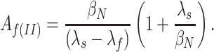 Here, λ_f is the faster relaxation eigenvalue that approaches −β_N at very negative voltages.

Secondly, some of the gating current measurements that we report were made with Cs⁺ replacing K⁺ in the bath. Cesium was originally used in many of our recordings since it is much less permeant in Shaker channels (Heginbotham and MacKinnon, 1993). However, Cs⁺ was observed to cause small changes in the properties of the gating currents at intermediate voltages (near −50 mV): Cs⁺ shifts, by −15 mV, the voltage range where a slow exponential component appears in the on gating current, and also shifts, by −15 mV, the prepulse voltages after which off gating currents begin to decay slowly. Since these phenomena are associated with channel opening (Bezanilla et al., 1991, 1994; Zagotta et al., 1994 a), we take these changes to mean that Cs⁺ alters some of Shaker's late gating transitions. Cs⁺, however, apparently does not alter the early gating transitions. Parallel measurements of gating currents made with bath K⁺ and Cs⁺ showed that gating currents induced by voltage pulses between −73 and −113 mV are unaffected by bath Cs⁺. Our analysis of gating currents at V ≤ −93 mV thus includes data obtained in Cs⁺ as well as K⁺ (Fig. 6 A). It should be noted that the liquid junction potential in the Cs⁺/NMDG⁺ solutions (−12 mV) was essentially the same as that for K⁺/NMDG⁺ solutions.

Figure 6.

Estimates of β₁ and β_d. (A) Gating currents elicited by voltage steps between −93 and −153 mV. The current recorded at −93 mV (top) reflects the on current measured after a voltage step from −133 mV; the currents recorded at the −153-, −133-, and −113-mV test voltages reflect the off current measured after voltage steps from −93 mV. Currents were fitted to a single exponential (smooth curves) to estimate a decay time constant τ. Patch w249. (B) To estimate β₁, the τ values derived from the currents in A were fitted to an exponential (solid curve), yielding β₁(0) = 200 s⁻¹ and q _β1 = −0.48 e₀. (C) The off gating current measured at −93 mV after a 2-ms depolarization to −33 mV was fitted to a single exponential with τ = 0.82 ms. This time constant is similar to the reciprocal of the value of β₁ at −93 mV (0.77 ms) estimated in B, consistent with β_d being similar to β₁ at −93 mV.

Nonstationarities in channel behavior.

Sigg et al. (1994a) have reported that the decay of Shaker's ionic tail currents recorded in excised membrane patches slows by a factor of ∼3 during the first several minutes after patch excision. We observed a similar time-dependent slowing in WT's tail currents. In eight patches, tail currents at −93 mV recorded at least 6 min after patch excision had decay time constants that were 2.9 ± 1.1-fold longer than tail currents recorded less than 1 min after patch excision. Time-dependent changes were also observed in the decay of WT's off gating currents after large depolarizations, which also reflect the kinetics of channel deactivation (Bezanilla et al., 1994; Zagotta et al., 1994 a). For the analysis of the macroscopic ionic tail currents and off gating currents, we therefore limited the analysis of tail currents to those measured at least 6 min after patch excision, when most of the time-dependent effects were apparently over. In seven patch recordings, in which tail currents were measured at different times up to 11 min or more after patch excision, the time-dependent slowing effect occurred with a time course that was approximated by a single exponential with τ = 6.2 ± 1.5 min.

No time-dependent effects were observed for any other macroscopic current properties. In three patches in which large changes in tail current decay rates occurred, the equilibrium voltage dependence of open probability never shifted by >3 mV and no significant changes in the measured activation time constants (at V ≥ −53 mV) were observed. We observed no nonstationary behavior in WT's single channel activity.

Slow inactivation.

A final potential problem for the interpretation of the macroscopic current time courses was slow-inactivation gating (Hoshi et al., 1991; Lopez-Barneo et al., 1993). In recordings made with 4–8-s voltage pulses to between −53 and +67 mV, macroscopic ionic currents decayed with voltage-independent kinetics that were fitted by the sum of two exponentials with time constants (at −13 mV) of 70 ± 13 and 870 ± 76 ms (n = 7); the 70-ms component comprised 26 ± 19% of the total amplitude. The slow inactivation time course was much slower than most, but not all, phenomena associated with activation gating. Thus, in the fits of exponentials to the channel opening time courses that are reported, an additional exponential component was always added that reflected the 70-ms component of the slow inactivation process.

results

The goal of this study is to identify kinetic transitions in activation gating and assign rate constants for the WT channel. Experiments were designed to isolate, as much as possible, the rates of individual steps in the activation process. In the first studies that we describe, we make use of data obtained at voltage extremes to study kinetic constants. We consider forward rates, assigning values and voltage dependences to the first forward rate α₁, the limiting rate at large positive potentials α_p, and the final opening rate α_N. An estimate for the voltage dependence q _αd of intermediate steps is also obtained. Similarly, the first and the last two backward rates β₁, β_N, and β_N-1 are determined, along with an estimate of the “average” rate of intermediate steps β_d. In the second group of studies, we characterize the transitions to several channel-closed states that are distinct from those traversed in the depolarization-induced activation process.

General Framework

We assume a discrete, homogenous Markov model for activation gating. Thus, activation is taken to involve transitions between discrete closed and open states separated by large energy barriers. For a sequential gating scheme, this framework can be depicted as

The forward and backward rates α_i and β_i are taken to be exponential functions of the membrane potential V, scaled by the partial charges q _αi and q _βi,

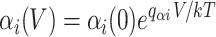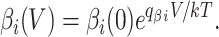1

(Terms with higher powers of V in the exponent are not included because any charge movement with the expected properties, if present, is very small; see Sigworth, 1994.) The gating charge movement accompanying a transition from state i − 1 to state i is then given from the partial charges as

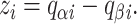2

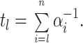
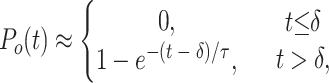
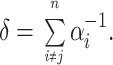
Within this framework, we estimate the forward and backward rate constants α_i and β_i for various gating transitions. Many of the current measurements were made at voltages where we could presume that either forward or backward rates predominate. Following Zagotta et al. (1994 a), we define three voltage ranges. Forward rates are presumed to predominate in the depolarized voltage range, where WT's equilibrium P _o and charge movement Q saturate. In WT's P _o − V and Q-V relations in Fig. 1, this appears to occur above −20 mV. (Although small changes in channel P _o continue at higher voltages, this property reflects the voltage dependence of a transition to a state that is not in the activation path and which carries only ∼0.3 e₀ of charge; Zagotta et al., 1994 a.) Backward rates are presumed to predominate at all voltages where most channels reside amongst the earliest closed states at equilibrium. These hyperpolarized voltages were taken to be V ≤ −90 mV because only 8% of WT's charge movement occurs negative to −90 mV. A third voltage range, activation voltages, between −90 and −20 mV, is the range in which WT's channel P _o and charge movement are undergoing most of their changes.

Figure 1.

Voltage dependence of relative channel open probability P _o and charge movement Q. Relative P _o estimates (▪) at V ≤ +67 mV were derived from measurements of ionic currents made using a double pulse protocol, in which currents were measured at a fixed amplitude voltage pulse (at −13 or +7 mV) that followed different test pulses. The values at +107 and +147 mV were obtained by measuring the magnitude of the current relaxation elicited by voltage jumps from +67 mV (in experiments similar to those illustrated in Fig. 12 A). Each plotted value reflects one to eight experiments. Relative Q estimates (○) were obtained as described previously (Schoppa et al., 1992), by numerically integrating the on gating current at each voltage. Each value reflects three to five experiments. The vertical dashed lines at −20 and −90 mV mark the boundaries of the defined hyperpolarized (V ≤ 90 mV), activation (−90 mV < V < −20 mV), and depolarized (V ≥ −20 mV) voltage ranges.

Given the special condition that all of the backward rates in Scheme SI are negligible, information about the forward rate constants in any sequential scheme can be obtained from a simple analysis of the time course of the open probability. At depolarized voltages, where we assume β_i → 0 for all i, the mean latency to arrive at the open state O _N is given by

3

Scheme I.

Now suppose that one of the rates, α_j, is much smaller than the others. Then the time course of channel activation can be approximated by the exponential function

4

with time constant τ = α_j ⁻¹ and with a time delay equal to the latency due to the other steps,

5

The approximate time course given by Eq. 4 has a mean latency that is equal to t _l; however, the time course is correct only as the limiting rate α_j becomes much smaller than the other rates. Useful estimates of the limiting rate and of δ can nevertheless be obtained from fits of Eq. 4 when the limiting rate differs little from the other rates. This is illustrated in Fig. 2, where fits were made to the “upper half” of the time course, starting at the time when P _o is equal to half of the final value. In Fig. 2 A, an “n ⁴” scheme where the next slowest rate is only twice that of the slowest one, the limiting rate is estimated with 11% error, while δ is estimated within 1%. Fig. 2 B demonstrates the worst case, in which no rate constant is smaller than the others. Here, the limiting rate is underestimated by a factor of two, while the error in δ is only 20%. Similar deviations between the measurements and theory are obtained from sequential schemes with more transitions. For an “n ⁸” scheme, the deviations in the measured and predicted τ⁻¹ and δ are only 13 and 1%, respectively; for eight equivalent rates, the deviations in τ⁻¹ and δ are 61 and 13%. These results suggest that fits of Eq. 4 to activation time courses for sequential models can yield reasonable first-pass estimates of the rate-limiting rate constant, though this rate will tend to be underestimated in cases where several rates are comparable in magnitude. Information about the other transitions is also obtained with surprisingly good accuracy from the delay value.

Figure 2.

Fits of a single exponential function and delay (Eq. 4) to the time course of open probability P _o predicted by different models. (A) Fits to the time course of P _o (solid curve) from the n ⁴ scheme Note that the order of rate constants in this scheme does not influence the time course. A fit of Eq. 4, taking only points where P _o ≥ 0.5, is shown as the dotted curve; it yields τ⁻¹ = 0.89 and δ = 1.09. The values expected from the approximate theory, τ⁻¹ = 1 and δ = 1.083, yield the dashed curve. (B) Fits to the time course from the same scheme but with all four rate constants equal to 1. The fit (dotted curve, fitted for P _o ≥ 0.5) yielded τ⁻¹ = 0.53 and δ = 2.45; the expected values are τ⁻¹ = 1 and δ = 3 (dashed curve). (C) Fits to the time course of P _o from Scheme SII, in which each of four independent subunits undergoes two transitions, with the forward rate constants a ₁ and a ₂ equal to 1 and 4, respectively. The fit (dotted curve, fitted for P _o ≥ 0.5) yielded τ⁻¹ = 0.89 and δ = 1.38. The expected values are τ⁻¹ = 1 and δ = 1.37 (dashed curve); these were obtained from the mean latency to opening t _l that was computed by use of a recursive subroutine as the expectation value over all possible paths in Scheme SII of the sum of dwell times in states in each path. (D) Fits to the time course from Scheme SII with a ₁ and a ₂ both equal to 1. The fit (dotted curve) yielded τ⁻¹ = 0.71 and δ = 2.38; the expected values are τ⁻¹ = 1 and δ = 2.55 (dashed curve).

The approximation of Eq. 4 can also be used to obtain a simple characterization of dwell times during activation in branched models. Consider a model like that of Zagotta et al. (1994 b) in which four independent subunits each undergo two steps,

When this scheme is expanded, it is seen that there are many distinct paths (14 in all) leading from closed state C₀ to the open state O₁₄.

The mean latency t _l can be computed as a weighted average of the time spent in each path, with the weights being the probabilities of the paths. The time spent in each path is the sum of the dwell times in each state of the path.

Fig. 2 C shows an example of fits to the time course for this scheme in the case where a ₁ = 1 and a ₂ = 4, yielding t _l = 2.369 time units. The simple theory predicts τ to be equal to the reciprocal of the slowest rate, and the delay parameter to be given by δ = t _l − τ. A single-exponential fit (dotted curve) yields a value for τ⁻¹ that differs by 11% from the slowest rate, and a value of δ that differs only 1% from the theoretical value. Fig. 2 D demonstrates the most difficult case, in which a ₁ = a ₂. As in the corresponding case of a sequential scheme (Fig. 2 B), the error in the time constant is moderate, ∼30%, but the error in δ is small, <1%. Thus, the parameters of a fitted single-exponential function give surprisingly good estimates for the aggregate dwell times in branched models as well as in linear models.

Estimates of Forward Rates

Estimates of α₁.

The forward rate constant α₁ for the first transition was evaluated from the time courses of ionic currents and gating currents at depolarizing voltages, as illustrated in Fig. 3. Fits of the single-exponential function (Eq. 4) to the ionic current from the 50% amplitude level to its final value yielded the “activation time constant” τ_a and the activation delay δ_a (Fig. 3 A). From the exponential decay of gating currents at depolarized voltages, the time constant τ_on was determined (Fig. 3 B).

Figure 3.

Estimate of α₁. (A) Macroscopic ionic currents at −13 and +37 mV were fitted to a single exponential (smooth curves) to estimate an activation time constant τ_a. Extrapolating the fitted exponential to zero current yielded an estimate of the activation delay δ_a. Patch w312. (B) The decay of WT's on gating currents at the same voltages was fitted to a single exponential (smooth curves) to estimate the decay time constant τ_on . Patch w212. For the fitting, a baseline was first calculated from the mean current measured at the end of the voltage pulse (horizontal lines); the fitting began at the time point at which the current had decayed by 20% from the peak value. (C) The values of τ_a (▪) and τ_on (○) derived from the fitting have nearly equal values at voltages between −13 and +67 mV. Each data point reflects the average from two to eight experiments. Superimposed curve reflects the average voltage dependence of α₁, obtained by fitting the τ_a values between −13 and +67 mV in seven different patches. (D) Exponential fits of the activation time courses and on gating currents for a five-state sequential scheme, as depicted in the legend for Fig. 2 A. For these simulations, the rates for all but one of the transitions was set to be 4; the slowest transition had a rate constant equal to 1. The position of the slowest transition was varied to yield the different curves. The activation time courses (top) were identical for each of the conditions; these were fitted to an exponential (dotted curve), yielding an activation time constant τ_a = 1.04. The gating current time courses for each of the conditions (bottom), however, differed. For C₁ → C₂, C₂ → C₃ = 1, the decay of the currents (dashed curves) was not well described by a single exponential. For C₃ → C₄ = 1, the decay of the current (solid curve) was well described by a single exponential (dotted curve), but the fitted time constant τ_on = 0.69 was faster than τ_a. For C₀ → C₁ = 1, the decay time constant τ_on = 1.09 was similar to τ_a . (E) Exponential fits of the activation time courses and on gating currents for Scheme SII, with the forward rate constants a ₁ and a ₂ equal to 1 and 4, respectively, or with a ₁ = 4 and a ₂ = 1. The two cases yielded identical activation time courses (top), which were fitted to an exponential with τ_a = 1.12 (dotted curve). The two cases, however, yielded different gating currents (bottom). The decay of the current for the case of a ₁ = 1 and a ₂ = 4 (solid curve) was well described by a single exponential with a time constant τ_on = 1.05, similar to τ_a. The case of a ₁ = 4 and a ₂ = 1, however, yielded a more complex gating current decay time course, which, when approximated by a single exponential (dotted curve), yielded a decay time constant τ_on = 0.51 that was much faster than τ_a. In all simulations, each transition carried an equivalent charge movement.

It has been shown previously that Shaker's on gating current displays a rising phase (Bezanilla et al., 1994), which implies that the forward rate of the first transition is slower than subsequent transitions or that the first transition has less associated charge movement. The additional observation that τ_a and τ_on have similar values at voltages near 0 mV (Fig. 3 C) suggests that the first step is the slowest at these voltages, being rate limiting for both channel opening and the movement of the charge.

The relationship between τ_a and τ_on is shown for a five-state sequential gating scheme in Fig. 3 D. In these simulations, we set the rates of all but one of the transitions to be equivalent and fast, and varied the position of the slow step. Only the case in which the slow step was the first step does the gating current decay with a single exponential with a time constant τ_on that is nearly identical to the activation time constant τ_a. We also show the relationship between τ_a and τ_on for the branched model in Fig. 3 E (bottom). For the case in which we made the rate a ₁ of the first “subunit transition” slow and rate limiting, the τ_a and τ_on values are nearly equivalent; however, for the case in which a ₂ is slow, the τ_a and τ_on values differ by a factor of 2. The results of these simulations suggest that it is reasonable to take the similarity between τ_a and τ_on for Shaker to mean that the first gating step is indeed the slowest. Activation at depolarized voltages then mirrors channel deactivation at hyperpolarized voltages, where the similar off gating current and tail current decay time courses imply that the first steps in channel closing are the slowest at these voltages (Bezanilla et al., 1991; Zagotta et al., 1994 a).

An estimate of the voltage dependence of the first forward rate α₁ can be obtained from the τ_a or the τ_on values at voltages up to +67 mV (Fig. 3 C). The reciprocal of the τ_a values derived from ionic currents measured between −13 and +67 mV in seven different patches yielded α₁(0) = 1,200 ± 90 s⁻¹ and q _α1 = 0.36 ± 0.02 e₀. As derived from τ_a, the value of α₁ might be underestimated if, as in the case illustrated in Fig. 2 B, other transitions have very similar rates. However, the close correspondence of τ_a and τ_on argues against the presence of this error.

Estimate of α_p.

If one or more transitions have forward rates with smaller voltage dependences than α₁, one of these should be rate limiting at sufficiently high voltages, and should be reflected in the voltage dependence of τ_a at very large positive voltages. Thus, we obtained current recordings at voltages up to +147 mV (Fig. 4 A). The analysis of the channel opening time course at high depolarized voltages is complicated by the fact that the rising phase of the current is usually not well fitted by a single exponential. After a rapid rise, a slow “creep” up to the final value is observed at these voltages. In a more complete discussion of this phenomenon below, we will show that this slow component reflects an alternate activation path that a small fraction of the channels enter before opening. Here, to estimate the kinetics of the main activation path, the currents were fitted to the sum of two exponentials,

6

Figure 4.

Estimate of α_p. (A) The upper half of the macroscopic ionic current time course at +87 and +147 mV was fitted to one or two exponentials (Eq. 6), respectively, to estimate τ_a and δ_a (smooth curves). Two exponentials were required at +147 mV to account for a slow relaxation that corresponds to an alternate activation path. Patch w312. (B) Voltage dependence of τ_a and δ_a taken from current measurements in two different patches (left and right). The τ_a values display shallower voltage sensitivities at high voltages. The voltage dependence of the rate α_p was estimated from the τ_a values at V ≥ +87 mV (solid lines at V ≥ +87 mV). The δ_a values between −13 and +147 mV also become less voltage sensitive at high voltages. Estimates of the charge q that determines the voltage sensitivity of the delay at low and high depolarized voltages, respectively, were obtained by fitting an exponential to the δ_a values at V ≤ +67 and ≥ +87 mV (dashed lines). These charge values will be used in a following paper (Schoppa and Sigworth, 1998b ).

τ_a was taken to be the time constant of the faster decay, whose amplitude A _f accounted for ∼90% of the total. The log-transformed values of τ_a up to +147 mV from two patches are plotted in Fig. 4 B. These plots do not show the linear dependence on voltage expected if a single transition is rate limiting at all of the voltages; instead, the dependence of τ_a on voltage becomes increasingly shallow at high voltages. Zagotta et al. (1994 a) made recordings of activation time courses only at voltages up to +50 mV, so these authors did not observe this deviation from simple behavior.

Estimates of the forward rate α_p of the rate-limiting step at high depolarized voltages were obtained as the reciprocals of τ_a values derived from the ionic current time courses measured between +87 and +147 mV, yielding α_p(0) = 2,100 ± 100 s⁻¹ (n = 6) and q _αp = 0.17 ± 0.02 e₀. It is not clear where in the sequence of gating steps this rate-limiting step occurs. The time course of gating currents at these high voltages could provide some information about this, but we did not record gating currents in this voltage range.

Estimate of α_N.

Macroscopic ionic currents were measured with one additional voltage protocol to attempt to estimate the forward rate α_N of the very last step in the activation path (Fig. 5). A sequence of three voltage pulses was applied (Fig. 5 A): an initial depolarization to +47 mV to open most of the channels, a second pulse to a hyperpolarized voltage V _h (−153 mV in this case) of duration t _h to close a fraction of the channels, and a third pulse to +47 mV to reopen the channels that closed during the second pulse. In principle, for small enough t _h, channels should not have time to close to states beyond the first closed state, and the kinetics of channel reactivation should reflect the forward rate of the last transition in the activation path. This time course will be distinctly faster if the forward rate of the last transition is faster than that of the earlier gating steps. Zagotta et al. (1994 a) measured currents using a similar voltage protocol with t _h as small as 1 ms, but we employed second-pulse hyperpolarizations that were much shorter, as short as 70 μs. In our experiments, briefer hyperpolarizing pulses make the reactivating currents much faster (Fig. 5, A and B). Compared with the 400-μs activation time constant τ_a taken from the reactivation time course after a relatively long t _h = 1 ms hyperpolarization, single exponential fits of the reactivation time courses for shorter t _h yielded τ_a values of 300, 170, and 110 μs for t _h = 300, 150, and 70 μs, respectively.

Figure 5.

Estimate of α_N from a fast reactivation component. (A, top) WT's macroscopic ionic currents elicited by a triple-pulse stimulus, using a pair of depolarizations to +47 mV separated by a voltage step to a hyperpolarized voltage V _h = −153 mV. The displayed currents correspond to different hyperpolarization durations t _h between 70 and 1,000 μs. Tail currents during the second pulse were inward since the pipette solution contained 14 mM K⁺. Data were filtered at 15 kHz. Patch w448. (bottom) The same traces are shown, but expanded and time shifted to align the start of the test pulses. The “upper half” of the reactivating current relaxations for t _h = 70 μs and 1 ms have been fitted to a single exponential to estimate τ_a (smooth curves). (B) The dependence of the derived values for τ_a on the hyperpolarization duration t _h, shown for different hyperpolarization amplitudes V _h. Note that for each V _h, the fastest τ_a values appear to approach 100 μs. All data reflect the patch in A. (C) To demonstrate that the fast reactivating component is not a recording artifact, we compare the apparent fast reactivating current in A for t _h = 100 μs with two different simulated current traces reflecting Eq. 7. The solid and dashed smooth curves, respectively, correspond to x(t) being a single exponential with a fast time constant τ = 100 μs (the good fit) or a slower τ = 430 μs (the poor fit). The total amplitude (−39 pA) associated with x(t) was constrained by fitting the tail current at −153 mV in the same patch to the sum of two exponentials and determining the amount of decrease in current by 100 μs after the beginning of the pulse. The impulse response h(i) was determined by differentiating the step response measured at the 15-kHz bandwidth (see methods). (D) The fast reactivation time constant (τ_f) values at different voltages were fitted to an exponential (solid curves) to estimate the voltage dependence of α_N, yielding estimates for α_N(0) and q _αN for each of three patches (α_N(0) = 7,600, 6,800, and 6,500 s⁻¹ and q _αN = 0.19, 0.16, and 0.18 e₀). For each patch, τ_f was obtained from currents measured after a 150-μs hyperpolarization to −153 mV. The reactivation time course for t _h = 150 μs includes a small slow component (accounting for, on average, 14% of the time course) as well as the dominant fast component; the τ_f values reflect the fast time constant in fits of the reactivation time course to the sum of two exponentials:

Several lines of evidence suggest that these fast relaxations reflect genuine current changes due to gating and are not artifacts of the recording system. First, the single-exponential fits just described were performed while ignoring the first 60 μs of the pulse, which at the 15-kHz bandwidth is longer than the settling time of the recording system (see methods). Second, the hyperpolarization to −153 mV produces a fast “instantaneous” current change reflecting the large change in the driving force between −153 and +47 mV. In the reactivation time course after a 1-ms hyperpolarization in Fig. 5 A, this current change is clearly complete within 40 μs and distinguishable from the slower kinetics of the current changes during the reactivating pulse. As a final check, we simulated reactivating current time courses I(t) by convolving theoretical functions x(t) reflecting current changes due to gating, with the impulse response of the recording system h(i):

7

The impulse response h(i) was obtained by differentiating the step response at the 15-kHz bandwidth at which these currents were measured (see methods) and was evaluated for n = 15 sample intervals. An additional constraint in this analysis was provided by the fact that an amplitude for x(t) can be predicted given the measured tail current time course during the preceding hyperpolarization. When it is assumed that x(t) is a single exponential with a time constant of 430 μs, which is the τ_a value taken from the activation time course during the first voltage pulse, I(t) poorly reproduces the data; but an exponential x(t) with a time constant of 100 μs accounts for the current time course very well (Fig. 5 C).

The 100-μs time constant at +47 mV is much faster than the reciprocal of the values that we calculate for both α₁ and α_p at +47 mV (430 and 400 μs, respectively) and thus reflects a distinct forward rate. It is difficult to prove that it is the very final step that is reflected by this time constant. More careful measurements using shorter hyperpolarizations might have revealed an even faster reactivation component associated with a later step. Nevertheless, consistent with the fast component reflecting the final step is that the effect of shortening t _h on the measured reactivation time constant appears to saturate at a value near 100 μs by the shortest −153-mV hyperpolarizations used (Fig. 5 B). The same saturating relationship between t _h and τ_a is observed when V _h is varied between −93 and −193 mV, which may be expected to produce varying occupancies in the closed states near the open state.

We define the activation time constant τ_a observed for the shortest hyperpolarization (t _h = 70 μs) to be the fast reactivation time constant τ_f reflecting the final forward rate α_N. The reciprocal of τ_f at +47 mV gives α_N(+47) = 9,100 s⁻¹. The voltage dependence of α_N was evaluated by varying the voltage of the test depolarization after a short duration hyperpolarization. From the voltage dependence of τ_f in this and two other patches (Fig. 5 D), we estimate α_N(0) = 7,000 ± 300 s⁻¹ and q _αN = 0.18 ± 0.01 e₀.

Estimate of q_αd.

The long delay in Shaker's channel opening time course (Zagotta et al., 1994 a) is expected to reflect the forward rates of a large number of transitions. While we were unable to determine directly the forward rates of most of the transitions that come between the very first and last transitions, information about the partial charges q _αd associated with the forward rates of these intermediate transitions is available from the voltage dependence of the delay δ_a in the channel opening time course (Fig. 4 B). The δ_a value represents the sum of contributions from multiple steps; its voltage dependence is not well fitted by a single exponential across the wide voltage range, which is consistent with transitions with forward rates with different voltage dependences predominating at different voltages. Nevertheless, to approximate the partial charges of a large number of these transitions here, the δ_a values between −13 and +147 mV were fitted to a single exponential (not shown), which yielded a charge estimate of 0.25 e₀ for q _αd.

Estimates of Backward Rates

Estimates of the voltage dependences of the backward rates of three transitions were obtained from the kinetics of macroscopic ionic and gating currents at hyperpolarized voltages.

Estimate of β₁.

The small fraction (<8%) of the total charge movement that occurs at voltages negative to −90 mV (Fig. 1) is consistent with the idea that at these voltages channels reside among the earliest closed states at equilibrium. If it is assumed that at −93 mV, most channels reside in either the first or second closed states, the off gating currents measured with voltage pulses from −93 mV to more hyperpolarized voltages will decay with a time course given by the backward rate β₁ of the first transition. Consistent with the expected two-state behavior, the measured currents (Fig. 6 A) rise instantaneously and have a single exponential decay that becomes faster at more hyperpolarized voltages. The time constants of the single exponentials fitted to these gating currents (Fig. 6 B) in three patches yielded an estimate for a backward rate of the earliest gating step β₁(0) = 190 ± 60 s⁻¹ and q _β1 = −0.53 ± 0.03 e₀. Numerous reports of Shaker's gating currents exist in the literature (Bezanilla et al., 1991, 1994; McCormack et al., 1994; Zagotta et al., 1994 a), but none of these include gating currents measured with voltage steps between different hyperpolarized voltages, which are required to estimate β₁.

The estimates of the backward rate β₁ obtained here and the forward rate α₁ obtained earlier can be compared with the Q-V relation. The charge of the first step z ₁ = q _α1 − q _β1 should match the steepness of the exponential Q-V relation at extreme negative voltages. Measurements of Q obtained between −133 and −83 mV were used, where Q/Q _max ≤ 0.13. Fitting the average data to an exponential function of voltage yielded an estimate of the first transition valence of z _Q = 1.1 e₀ (not shown). This z _Q estimate is similar to the estimate z ₁ = 0.9 e₀ obtained from the voltage dependences of the forward and backward rates.

Estimate of β_d(−93).

It has been previously shown that Shaker's off gating currents after large depolarizations have a rising phase and decay kinetics dominated by the slow kinetics of channel closing from the open state (Bezanilla et al., 1991; Zagotta et al., 1994 a). However, the off current kinetics after short depolarizations that fail to open channels are much more rapid, presumably reflecting the relatively rapid backward kinetics of the transitions that come before the last transition (Zagotta et al., 1994 a). We use this rapid off current time course here to obtain an approximate estimate β_d for the backward rate of intermediate transitions. Fig. 6 C illustrates the off current measured after a short 2-ms depolarization to −33 mV. From the time integral of the gating current at this voltage, we estimate that 80% of the total gating charge movement occurs by the end of the 2-ms depolarization, indicating that most channels reside in relatively late activation states; however, from the channel opening time course, we estimate that only 15% of the channels are open. Exponential fits of the off currents after the 2-ms depolarization to −33 mV in two patches yielded time constants of 0.82 and 0.62 ms.

The decay of this off current reflects the contribution of the backward rates of many transitions, including the transitions between intermediate states that are preferentially occupied at the end of the prepulse depolarization, and also β₁ of the first transition. The decay time constant of the current is in fact indistinguishable from the reciprocal of β₁ at −93 mV (0.77 ms), suggesting that the rate of the intermediate steps β_d is similar to β₁ at −93 mV. This analysis gives a rough estimate of β_d(−93 mV) = 1,300 s⁻¹.

Estimate of β_N.

Zagotta et al. (1994 a) made estimates of the channel closing rate β_N from macroscopic ionic tail currents measured between −60 and −140 mV. For our estimates of β_N, we chose to use tail currents measured at even more negative voltages. While the position of the Q-V relation on the voltage axis would suggest that most of the forward rates are negligible in the hyperpolarizing voltage range (≤−93 mV), it has been shown above that the forward rate of the last transition α_N is considerably faster than the forward rates of the preceding transitions, and could have values at voltages near −93 mV that are comparable to backward rates. Indeed, according to our fits, α_N(−93) = 3,600 s^{− 1} is greater than β₁(−93) = 1,300 s^{− 1}. Considering a partial scheme consisting of the last three states of Scheme SI,

the channel deactivation time course at these voltages might involve many reopenings from state C_N-1 before closing further to state C_N-2. The large forward rate of the last transition implies that estimates of β_N must be obtained from currents measured at voltages more negative than −93 mV.

Inward tail currents were measured between −153 and −203 mV using 14.3 mM external K⁺ (Fig. 7 A). One criterion to determine that the tail current time course entirely reflects the channel closing rate β_N is that it should be well fitted by a single exponential, but even at the most negative voltages, the tail currents were poorly fitted by a single exponential. Assuming that the complicated channel deactivation time course reflects channel reopenings from the last closed state in the activation path, as reflected in Scheme SIII, estimates of β_N could nevertheless be obtained by fitting the tail currents to the sum of two exponentials:

8

Scheme III.

with the faster time constant τ_f reflecting β_N at sufficiently negative voltages.

In practice, only tail currents at V ≤ −153 mV were considered in this analysis. At these voltages, τ_f displays the single-exponential dependence on voltage expected for β_N (Fig. 7 B). Additionally, the amplitude A _f (Fig. 7 C) of the fitted fast exponential increases monotonically below −153 mV, expected for a tail current time course that reflects channel reopenings from the last closed state in the activation path but reflecting increasingly fewer reopenings at more negative voltages. The reciprocal of the τ_f values at different voltages below −153 mV from five separate patches yielded estimates of β_N(0) = 290 ± 90 s⁻¹ and q _βN = −0.50 ± 0.04 e₀.

Estimate of β_N-1.

If WT's channel deactivation time course is determined at most voltages by the channel closing rate and by reopenings from the last closed state C_N-1, this time course provides one way to estimate the backward rate β_N-1 from the pentultimate state. A second measure of β_N-1 is provided by the reactivation time courses (Fig. 5 A). The amplitude of the fast reactivation component should reflect the occupancy in C_N-1 during the preceding hyperpolarization. The voltage dependences of the rates of the transitions out of C_N-1, including β_N-1, will determine the way in which this amplitude varies with the duration t _h and amplitude V _h of the preceding hyperpolarization.

Fig. 8 A illustrates the strategy we used to estimate the size of the fast component in the reactivation time course. In this analysis, we used an observation made in a different experiment, that changing the amplitude of a pre-pulse has a negligible effect on the kinetics of the final approach of the measured ionic current, estimated by τ_a. (These data are not shown here, but see Fig. 18 B in Schoppa and Sigworth, 1998b ). This result suggests that a reasonable approximation to the fast and slow components in the reactivation time course is the function

9

Figure 8.

Estimate of β_N-1. (A) Separation of the reactivation time course into fast and slow components. Selected current traces in Fig. 5 A are shown for t _h between 100 μs and 1 ms. The time course of the fast component, reflecting channels reopening from C_N-1, and the slow component, reflecting channels reopening from all closed states that precede C_N-1, were approximated by fits of Eq. 9 (smooth curves). In the fitting, the value for α_N was fixed to the mean value derived from the reactivation time courses in Fig. 5 D. From the slow component, we derived an estimate of the delay δ_a (shown for t _h = 1 ms; dashed curve). (B) The occupancies in C_N-1 derived from the reactivation time courses, as well as tail currents (C), were fitted to Scheme SIII (superimposed smooth curves) to obtain estimates of β_N-1 and β_N. The occupancy p _N-1 in C_N-1 for different amplitude V _h and duration t _h was obtained from fits of Eq. 9 to the reactivation time course as p _N−1 = A _f/ (I _inst + A _f + A _s); that is, taking A _f to reflect the amplitude of current due to the return of channels from C_N-1 to the open state. This expression for p _N-1 is approximate, but is expected to hold in this case. Each of the data points reflects one to four experiments. The parameter estimates obtained were: β_N(0) = 150 s⁻¹, q _αN = −0.57 e₀, and β_N-1 (0) = 320 s⁻¹, q _βN-1 = −0.30 e₀. In the fitting, α_N was fixed to mean estimate value for α_N (Fig. 5 D); all channels were assumed to reside in the open state at the beginning of the test pulse.

Varying the exponent r in the third term (while allowing it to take fractional values) yields an opening time course with varying amounts of delay, but with a nearly invariant final approach. The fits of Eq. 9 to the reactivation time courses in Fig. 8 A have been separated into the respective fast and slow components. Increasing t _h from 100 to 200 μs yields a larger fast current, but the magnitude of this current decreases with even longer t _h, reflecting channels entering closed states that precede C_N-1 during the hyperpolarization. For the slow component, increasing t _h produces a monotonic increase in amplitude, and also a longer delay, reflecting channels entering into relatively early closed states.

Estimates of β_N-1 were then obtained by simultaneously fitting the three-state Scheme SIII to the time course of occupancy in C_N-1 (Fig. 8 B), estimates of which were derived from the amplitude of the fast reactivation component, as well as to tail currents (Fig. 8 C). We restricted our analysis to voltages lower than −90 mV, where we assume that the tail current and occupancy time courses are functions of just α_N, β_N, and β_N-1; that is, we take the reverse rate β_N-2 to be much greater than the forward rate α_N-1, so that only reverse transitions occur out of C_N-2. In the fitting, α_N was fixed to the estimate obtained in Fig. 6, but β_N was allowed to vary along with β_N-1. Good fits of the tail current time courses and the derived occupancy estimates are obtained with the parameter estimates for β_N and β_N-1 indicated in the legend. The smaller estimate for the charge q _βN-1 compared with q _βN accounts for the relatively higher occupancies in C_N-1 at the most hyperpolarized voltages (Fig. 8 B). We note that the derived estimates for β_N-1(0) and q _βN-1 may be too large if the assumption that β_N-2 is much greater than α_N-1 at V ≤ −93 mV is not valid.

The fits of the data in Fig. 8 to Scheme SIII are expected to provide a more reliable estimate of β_N than that derived from fitting the tail currents to the sum of two exponentials in Fig. 7. However, the estimate for β_N derived from the fits of Scheme SIII is nearly identical to that derived directly from the tail currents (Fig. 7 B). Additionally, the fast tail current component predicted by Scheme SIII has approximately the same amplitude as the faster component in the two-exponential fits of the tail currents (Fig. 7 C). These observations confirm our direct estimates of β_N.

Estimate of q_βd.

A measure of the partial charge q _βd associated with the backward rates of intermediate transitions was obtained from measurements of macroscopic ionic currents, using a strategy that is analogous to that used above to estimate q _αd. In that case, the voltage dependence of the delay in channel activation gave a rough estimate of the voltage dependence of the underlying rate constants of intermediate transitions. Here we measure the activation delay as initial state occupancies are varied using repolarizing pulses of duration t _h and amplitude V _h that follow an initial depolarization that loads the channels into the open state. Let the initial occupancy of state i be p_i, and let α_i be the forward rate from state i to state i + 1. Then Eq. 5 can be generalized to give the delay with arbitrary occupancies,

10

where again we assume the unidirectional sequential Scheme SI and that rate α_j is rate limiting. The dependence of δ_a on t _h will reflect the time dependence of the occupancies during the hyperpolarizing pulse and therefore depend on the backward rates of the transitions that contribute to the delay. The dependence on V _h of this accumulation will be a function of the partial charges that determine these backward rates.

The analysis of the accumulation of the delay requires defining three parameters. The first is the delay δ_a derived by fitting a single exponential to the slow component in the reactivation time course (Fig. 8 A), which has been approximated by the second term in Eq. 9. The second parameter is τ_acc(V _h), which is the time constant of a single exponential fit to the dependence of δ_a on t _h at a given V _h (Fig. 9). The third parameter is the estimate of the charge q _acc that reflects the voltage dependence of the accumulation of the delay, obtained by fitting the τ_acc values to an exponential function of V _h (Fig. 9 B).

Figure 9.

Estimate of q _βd. (A) Values of δ_a taken from the slow component in the reactivation time courses (shown in Fig. 8 A), for hyperpolarizations of different amplitude V _h and duration t _h. For each V _h, the time course of the accumulation of the delay for increasing t _h was approximated by a fit of the δ_a values to a single exponential (solid curves), yielding τ_acc. The fitted exponential was constrained to begin at zero. The amplitude was fixed to have the value of δ_a measured from the current elicited by the first of the three voltage pulses in the triple pulse protocol (starting from a −93-mV holding potential). For V _h = −113, −153, and −193 mV, the amplitude was multiplied by a scaling factor to account for the fact that prepulses to voltages more negative than −93 mV yield a slightly longer delay in the channel opening time course. All data except for V _h = −93 mV come from the same patch (w448). (B) Values of τ_acc for different V _h were fitted to an exponential (solid curve) to estimate a charge q _βd = −0.24 e₀. Values reflect pooled measurements made in four different patches.

Changing the hyperpolarization voltage V _h from −93 to −193 mV (Fig. 9 A) causes the delay to accumulate more quickly, which is expected for backward rates with associated negative partial charges. Notably, however, the time course of the accumulation of the delay is only about twice as fast at −193 as at −93 mV, consistent with backward rates having only small partial charges. Evaluating reactivation time courses for various V _h and t _h in four patches, the τ_acc(V _h) values across the voltage range showed a voltage dependence corresponding to a charge of −0.24 e₀ (Fig. 9 B), which we take as an estimate of q _βd. Additionally, we can use this estimate of q _βd to derive an estimate of the rate β_d(0) at 0 mV, given the estimate of β_d(−93) = 1,300 s⁻¹ obtained above from gating currents. This gives β_d(0) = 540 s⁻¹.

Transitions to States that Are Not in the Activation Path

Up to this point, we have characterized the transitions that the Shaker channel undergoes in the depolarization-induced activation process. However, Hoshi et al. (1994) have shown from Shaker's single channel data that there are at least two additional closed states, called C_f and C_i, into which the channel enters only after it has opened. The state C_f corresponds to a predominant, fast 200–300-μs component in their single channel closed dwell-time histograms at depolarized voltages, and the other closed state C_i accounts for a voltage-independent, 1–2-ms component in the closed time histograms at depolarized voltages. In the following, we use a combination of single channel and macroscopic current measurements to further characterize the transitions to these additional states.

We begin by outlining the general properties observed in our single channel measurements at depolarized voltages. As was observed by Hoshi et al. (1994), we find that the channel opens quickly after the beginning of a voltage pulse (Fig. 10 A) and remains open for most of the trace, occasionally closing briefly into short-lived closed states. Infrequently, the channel displays longer closures (see the third trace at +67 mV). The closed time histograms constructed from our single channel activity are always fitted by a mixture of three exponentials (Fig. 10 B), including one large-amplitude component with a very fast (τ₁ = 40–100 μs) time constant, a second component with an intermediate amplitude and duration (τ₂ = 200–500 μs), and a third component with a 1–3-ms time constant (τ₃) and a very small amplitude (comprising ∼1% of the closures). Our fit of two exponentials to closures with durations of <500 μs differs from the single exponential fitted to these closures by Hoshi et al. (1994). It is difficult to interpret the voltage dependences of the two faster closed time components (Fig. 10 D), since the rapid closures are near the limit of time resolution and, additionally, the two rapid closed-time components are not well resolved from each other. The third, slowest component has a voltage-independent duration and corresponds to the C_i closures observed by Hoshi et al. (1994).

Figure 10.

Single channel activity at depolarized voltages. (A) Traces of single channel currents elicited by voltage pulses from −93 mV to different test voltages. The beginning of the voltage pulse is indicated by the vertical dashed line. Patches w265 and w276. (B) Closed dwell-time histograms from depolarizations in 40-mV increments between −13 and +147 mV. The histograms were fitted to the sum of three exponentials; dashed curves correspond to each of the fitted exponential components. The number of events in each histogram is ≥605. (C) The open dwell-time histograms at the same voltages were well fitted by a single exponential. (D) The time constants (τ₁, τ₂, and τ₃) of the fast, intermediate, and slow exponential components of the closed-time histograms have nearly voltage-independent values near 0.1, 0.3, and 2 ms. The τ₃ values were fitted to an exponential (solid line) to estimate the rate d from C_iN to the open state. Data points reflect pooled results from several patches. Time constant values from the fits of the histograms shown in B are indicated by the filled symbols. (E) The time constants τ₀ of the single exponentials fitted to the open times display little voltage dependence. Also, the large discrepancy between τ₀ and the reciprocal of the channel closing rate β_N (solid line) indicates that nearly all of the closures at depolarized voltages are to states that are not in the activation path. The τ₀ values from the fits of the histograms shown in C are indicated by the filled symbols. (F) An estimate for the rate c from the open state to C_iN was derived by fitting an exponential (solid curve) to estimates of the frequency of C_i closures, corresponding to the τ₃ component in the closed dwell-time distributions. Frequency estimates were obtained from the measured channel open times normalized by the relative contribution of the C_i closures to the total number of measured closures. Values obtained from the histograms in B and C are indicated by the filled symbols. For the closed dwell-time histograms shown in B, the relative amplitudes A ₁, A ₂, and A ₃ of the fast, intermediate, and slow exponential components are as follows: at −13 mV, 0.74, 0.24, and 0.02; at +27 mV, 0.83, 0.16, and 0.01; at +67 mV, 0.79, 0.20, 0.02; at +107 mV, 0.83, 0.16, and 0.01; and at +147 mV, 0.85, 0.14, and 0.01.

As shown previously (Hoshi et al., 1994), the open times (Fig. 10 C) are well fitted by a single exponential with time constants near 3 ms, consistent with the presence of a single open state. The measured open times display little voltage dependence (Fig. 10 E). No effort was made to correct the open times for missed fast closures because the missed event correction would rely on the amplitude and time constant estimates for the fastest closures, which are quite unreliable.

Characterization of the Transitions to C_i

The first new property that we assign to C_i is that it is a state that can be entered from not only the open state but also from closed states in the activation path. This property for C_i is required by the fact that C_i contributes to occasionally observed long first latencies to channel opening at depolarized voltages.

An instance in which the channel enters into a long-lived closed state before it opens is evident in the second trace at +67 mV in Fig. 10 A. Entries into long-lived closed states before first opening are also apparent in the shape of the cumulative first latency histogram (Fig. 11 A), which displays a gradual rise superimposed on the dominant faster component. The same slow component was also usually observed in the time course of macroscopic ionic currents at high depolarized voltages (V ≥ +67 mV; Fig. 4 A). While a single-exponential fit may account for the time course for even a complex gating scheme depending on the way that the fitting is performed, the observed deviation from a single-exponential time course in the final approach of the current in our fits is good evidence that individual channels are traversing different rate-limiting steps to opening. The observed two components in our time courses apparently are not, however, due to differences in the initial conditions for different channels, because the size of the slow component in the macroscopic current does not change with a very hyperpolarizing prepulse to −143 mV (in three patches; data not shown); this prepulse is expected to preload virtually all channels into the very first closed state. The slow component is also probably not due to modal gating, as it was found in one single channel patch recording that there was no apparent pulse–pulse correlation in the appearance of long first latency. Instead, we take the presence of two components in the final approach of the ionic current to imply that there are two pathways to channel opening; that is, a fraction of channels pass through closed states in a slow path that is distinct from the main activation path.

Figure 11.

C_i states can be entered from closed states in the activation path. (A) The upper half of the cumulative first latency histogram at +67 mV was fitted to the sum of two exponentials (Eq. 6; solid curve), yielding the indicated τ_a, τ_s, and relative A _s values. The dashed curve reflects just the fast component in Eq. 6. The difference in the amplitude of the two curves reflects A _s. Patch w265. (B) The time constants τ_s obtained in the fits of Eq. 6 to first latency distributions (▪) and macroscopic ionic currents (○) at V ≥ +67 mV have values of 1–3 ms. Only two of the single channel experiments had enough traces that a slow component could be convincingly discerned in the latency histogram. However, 21 of 28 relatively smooth macroscopic ionic current time courses at V ≥ +67 mV (measured in seven patches) displayed an unambiguous slow component. The τ_s values were fitted to single exponential (solid curve). The derived charge estimate q = −0.14 e₀ indicates that the time constant of the slow component is nearly voltage independent. (C) The relative magnitude of the slow exponential component A _s/(A _f + A _s) is also nearly voltage independent. These values were fitted to an exponential, yielding q = 0.07 e₀.

In fits of two single-channel first latency histograms at V ≥ +67 mV to the sum of two exponentials (Eq. 6), the fitted slow exponential had time constant τ_s values of 1.6 and 1.8 ms (Fig. 11, A and B), similar to the 1.9 ± 0.5-ms mean duration of the τ₃ component in the closed dwell-time histograms at the same voltages (n = 3; Fig. 10 D). Fits of 21 macroscopic ionic current time courses to Eq. 6 yielded τ_s = 1.5 ± 2 ms, also similar to τ₃. (The time course of the slow component in the macroscopic ionic current can be compared with τ₃ because backward rates at high voltages are negligible, making the ionic current have essentially the same time course as the cumulative first latency histogram; Hoshi et al., 1994.) We take the similarity in the latency time constant and τ₃ to imply that the long latencies to opening reflect sojourns in the same family of states as the C_i closures that follow the first opening, except these sojourns in C_i are made from closed states in the activation path. The experiments of Hoshi et al. (1994) were not able to discriminate transitions into C_i before opening because their single channel measurements were not made at sufficiently high voltages; at lower voltages, the kinetics of the transitions through this secondary activation path are not substantially slower than the kinetics of the main activation path.

The slow component accounts for on average ∼10% of the total current relaxation (Fig. 11 C), implying that an opening channel has a 10% chance of entering one of a family of C_i states from closed states in the activation path before opening. For example, in the following scheme,

the opening channel might move from the resting state C₀ into C_N-1, and then into C_iN-1 and C_iN, before reaching the open state O_N. From which particular set of closed states the channel can enter the C_i states remains unclear. Scheme SIV does not include transitions between C_iN and C_f, because we prefer a simple model for these states.

Scheme IV.

If it is assumed that most of the C_i closures observed at equilibrium at depolarized voltages correspond to sojourns in the state C_iN, which is entered directly from the open state, we can use the closed and open dwell-time histograms to assign estimates for the rates c and d of this transition. The values of the time constants fitted to the C_i closures at different voltages give an estimate for the rate d from C_iN to the open state (d(0) = 300 s⁻¹ and q _d = 0.07 e₀; Fig. 11 D). The open times and amplitude of the C_i closed time component (Fig. 10 F) give estimates for the rate c from the open state into C_iN (c(0) = 5 s⁻¹ and q _c = 0.09 e₀). This estimate for c is an upper limit, if some of the C_i closures observed under equilibrium conditions reflect sojourns in states entered from closed states in the activation path.

Evidence for C_f1 and C_f2

We next evaluate the transitions that correspond to the two rapid components of the closed-time histograms in Fig. 10 B. Since Hoshi et al. (1994) have shown that many of the rapid closures at depolarized voltages are to states that are not in the activation path, our starting hypothesis will be that the two rapid components correspond to two different such states: C_f1 and C_f2. The alternate possibility is that one of the components corresponds to closures in the activation path (e.g., to the last closed state C_N-1). We can address this second possibility by comparing the measured channel open times and the reciprocal of our estimated channel closing rate β_N (Fig. 10 E). At the most depolarized voltage where currents were measured (+147 mV), the measured channel open time (3 ms) is 60 times shorter than the expected value of 1/β_N = 180 ms at that voltage. (Were we to correct the open time for missed brief closures, the discrepancy with 1/β_N would be even larger.) This large difference implies that virtually all of the measured closures at this voltage reflect closures to states that are not in the activation path. Since the two rapid components of the closed time histograms at +147 mV comprise 73 and 25% of the total measured closures, both very much larger than the ∼2% component expected for closures to C_N-1, we take both components to reflect closures to states C_f1 and C_f2 not in the activation path.

While there are a number of different ways to model these two states, we suggest that C_f1 and C_f2 are states into which the open channel closes directly:

We cannot easily rule out alternative models (e.g., having channels in O_N close first into C_f2 and then into C_f1), but we choose Scheme SV because of its simplicity.

Scheme V.

Since the rapid closures in the single channel recordings are not well resolved, the parameter values derived from exponential fits to the histograms do not yield quantitatively reliable estimates of the rates associated with the transitions to C_f1 and C_f2. We nevertheless obtain rough estimates of these rates by using various strategies.

Estimating Rates for the Transition to C_f1

If the transition to either C_f1 or C_f2 carries any amount of charge, the rates for this transition can be estimated from the relaxation of macroscopic ionic currents that are elicited by a double pulse protocol. To achieve test currents that predominately reflect the transition to C_f1 or C_f2, prepulses are required that are large enough that virtually no channels reside in states in the activation path at the end of the prepulse. A comparison of the measured channel open times and the reciprocal of the closing rate β_N in Fig. 10 E indicates that at voltages ≥+7 mV, open times are approximately the same or shorter than 1/β_N; this would imply that much of the test current relaxation after prepulses above +7 mV reflects transitions to states outside the activation path.

Fig. 12 A illustrates an experiment in which we apply voltage steps from +7 to +127 mV, and also from +47 to +147 mV. These voltage jumps elicited small current relaxations with activation time constants of τ_r = 230 and 180 μs. The time course of the current relaxation at +147 mV (τ_r = 180 μs) is threefold slower than the fast reactivation time constant that corresponds to the last transition in the activation path (Fig. 5 D); this indicates that the observed current must reflect a transition that is distinct from the last activation transition. The observed relaxation also cannot reflect the transition to C_iN. Given the estimates for c and d assigned above, the transition to C_iN would contribute to a change in open probability ΔP _o << 1% during these voltage jumps, but the amplitudes of the relaxations correspond to ΔP _o ≥ 6% (see legend to Fig. 12). Thus, these relaxations almost certainly reflect transitions to C_f1 or C_f2, and we assign them to C_f1. Since these currents are recorded at depolarized voltages, we assume that the current time course mostly reflects the rate f ₁ from C_f1 to the open state, yielding estimates of f ₁(0) = 1,600 s⁻¹ and q _f1 = 0.2 e₀ (Fig. 12 B).

Figure 12.

Characterization of the transitions to C_f1 and C_f2. (A, top) Macroscopic ionic currents elicited by voltage steps between pairs of depolarized voltages. The smaller current (at both the prepulse and test voltages) reflects a voltage step from +7 to +127 mV, and the larger current reflects a voltage step from +47 to +147 mV. Data were filtered at 15 kHz. Patch w447. (bottom) The same traces are expanded to show just the current relaxation during the test pulse; zero time is the start of the test pulse. The current relaxations are fitted to a single exponential to estimate the time constant τ_r (solid curves). At +127 and +147 mV, the time constants are τ_r = 230 and 180 μs, respectively, and the amplitudes of the fitted exponentials are −32 and −21 pA. These amplitudes can be compared with the size of the rest of the test current (278 and 323 pA, respectively) to yield estimates of the change in P _o induced by these voltage steps (10 and 6%). (B) The rate f ₁ from C_f1 to the open state was estimated by fitting an exponential (solid curve) to the τ_r values (▪) taken from the current relaxations measured in the experiment in A and from similar measurements made in one other patch. (C) Estimates of absolute P _o at voltages between +47 and +147 mV were derived from the mean measured channel closed and open dwell times in the equilibrium single channel activity. The data points reflect measurements made in four patches. Absolute P _o apparently saturates near 0.9.

The value of the rate constant e ₁ for the entry into C_f1 can be determined using the amplitude of the current relaxation in the voltage jump experiment in Fig. 12 A. The 10% change in relative P _o induced by the voltage jump from +7 to +127 mV, together with the value for f ₁ derived above, gives e ₁ = 190 s⁻¹ at +7 mV (assuming that the transition to C_f1 is saturated at +127 mV). We assume that this transition is voltage independent.

The current relaxations in Fig. 12 A verify one feature of data presented earlier in this paper. In the voltage dependence of channel opening for Shaker (Fig. 1), P _o rises steeply to ∼80% of its maximal value, but displays a slow upward drift at higher voltages. The presence of the gradual rise, however, has been reported to be dependent on the method by which P _o is measured (Zagotta et al., 1994 a). The 12% change in relative P _o that we estimate to occur between +7 and +67 mV using the tail-current method for estimating relative P _o (described in the legend of Fig. 1) is, notably, similar to the 10% change in relative P _o induced by the voltage jump from +7 to +127 mV. In our modeling paper (Schoppa and Sigworth, 1998b ), we will use the shape of the P _o -V relation at depolarized voltages to help constrain the total charge associated with the transition to C_f1.

Estimating Rates of the Transition to C_f2

The relaxations of the macroscopic currents in Fig. 12 A that correspond to C_f1 → O have similar time-constant values as the intermediate duration τ₂ component of the single-channel closed dwell-time histograms at similar voltages (Fig. 10 D); at V > +100 mV, τ₂ is between 200 and 300 μs. If the transition from C_f1 corresponds roughly to the intermediate duration closures in the dwell-time histograms, the transition from C_f2 must correspond to the very rapid 40–100 μs closures. These closures are poorly resolved, but the short apparent time constant implies that the rate f ₂ from C_f2 to the open state is very rapid (near 10⁴ s⁻¹). Information about this transition can also be obtained from estimates of absolute P _o, which can be derived from the mean open and closed times in the single channel measurements (Fig. 12 C). From measurements obtained at voltages as large as +147 mV, the derived absolute P _o values apparently saturate near 0.9. The fact that P _o at very high voltages saturates at a value less than unity implies that the transition to C_f2 is nearly voltage independent (giving q _e2 + q _f2 ≈ 0.0). A saturating value of P _o = 0.9 implies a ratio of the two rates e ₂/f ₂ near 0.1, giving e ₂ ≈ 10³ s⁻¹.

discussion

In this and the following two papers (Schoppa and Sigworth, 1998a , 1998b ), we characterize activation gating for the normally activating Shaker channel (WT) and a mutant version of the channel to arrive at a relatively well-constrained activation gating model. In this first paper, we have undertaken a detailed analysis of the kinetics of WT's macroscopic ionic and gating currents and single channel currents in an effort to obtain estimates of several rate constants. Previous efforts at characterizing Shaker's activation gating process exploited experimental strategies that were similar to ours in order to isolate particular activation gating transitions (Hoshi et al., 1994; Zagotta et al., 1994 a; Bezanilla et al., 1994 a). However, we have gained new insights by analyzing the current time courses in novel ways and by extending the voltage range of the current measurements.

Estimates of Forward and Backward Rates for Transitions in the Activation Path

We have assumed that activation gating is described by a Markov process with transitions between discrete states separated by large energy barriers. Fits of exponentials to selected ionic and gating current time courses at extreme voltages yielded estimates of the rate constants depicted here.

For the forward rates, we have obtained estimates of the first forward rate α₁, the limiting rate at large positive potentials α_p, the final opening rate α_N, and an estimate of the partial charge q _αd that determines the voltage dependence of forward rates of intermediate steps. For backward rates, we have obtained estimates of the first and last two backward rates (β₁, β_N-1, and β_N), and an estimate of the backward rates of intermediate steps β_d. The values obtained are given in Table I. We have also extended on the work of Hoshi et al. (1994) by characterizing the transitions to several closed states that are not normally traversed before the channel opens. Hoshi et al. (1994) showed that there were at least two such states C_i and C_f; from an analysis of single channel data, we have shown that there are at least four such states. These results are summarized by Scheme SV above and the list of rate estimates in Table II.

Table I.

Estimates of Rate Constants for Transitions in the Activation Path

Rate (0 mV)		Partial charge
αl(0) = 1200 s−1		qαl = 0.36 e0
αp(0) = 2100 s−1		qαp = 0.17 e0
αN(0) = 7000 s−1		qαN = 0.18 e0
—		qαd = 0.25 e0
βl(0) = 190 s−1		qβl = −0.53 e0
βN(0) = 150 s−1		qβN = −0.57 e0
βN−1(0) = 320 s−1		qβN−1 = −0.30e0
βd(0) = 540 s−1		qβd = −0.24 e0

 

Table II.

Estimate of Rate Constants for Transitions to States Outside of the Activation Path

Rate (0 mV)		Partial charge
c ≤ 5 s−1		qc = 0.09 e0
d = 300 s−1		qd = 0.07 e0
e l ≈ 200 s−1		qe l ≈ 0
f l = 1600 s−1		qf l = 0.20 e0
e 2 ≈ 103 s−1		qe 2 − qf 2= 0
f 2 ≈ 104 s−1

 

It should be emphasized that the parameters q _αd, q _βd, and β_d(0) that we ascribe to intermediate transitions should be taken as quite rough approximations; these are shown in Scheme SVI with parentheses. The charge parameters q _αd and q _βd were derived from the delay in the channel opening time course, which reflects the composite properties of many transitions. These parameters are also somewhat difficult to interpret because transitions with the fastest forward rates contribute little to the delay. Thus, these charge parameters are not likely to reflect the partial charges associated with the most rapid transitions. However, the number of rates with partial charges similar to q _αd and q _βd is likely to be quite large. Zagotta et al. (1994 b) estimated that a minimum of five transitions are required to account for the delay in the ionic current time course; our own analysis gives a minimum estimate of seven transitions (Schoppa et al., 1998b), implying that at least six transitions contribute significantly to the delay.

Scheme VI.

Assumptions Used in the Derivation of Rate Constants

The accuracy of these rate estimates has relied on a number of assumptions, besides the assumption of a Markov process. The first of these is that our current measurements were made at sufficiently positive and negative voltages to yield unidirectional transitions, so that our current measurements reflect only a single microscopic rate constant. All but one of the forward rates were estimated from currents measured at V ≥ +67 mV, which is 80 mV higher than where the Q-V relation saturates, and all backward rates were estimated from currents measured at V ≤ −93 mV, where <8% of the charge movement occurs. While we cannot be certain that transitions are unidirectional at these voltages, our current measurements were made at more extreme voltages than those that have been published previously. Thus, for example, in the estimate of the channel closing rate β_N, our estimates are likely to be more reliable than those that have been reported previously.

The forward rate α₁ of the first transition was estimated from current measurements made at voltages between −13 and +67 mV. The reason for concern about voltage ranges for this estimate is the following. Whereas the equilibrium P _o -V and Q-V relations appear to saturate near 0 mV (Fig. 1), previous models for Shaker's gating (Bezanilla et al., 1994; Zagotta et al., 1994 b) have included at least one transition that has a relatively large backward rate at this voltage; the channel nevertheless opens due to the driving action of a later forward-biased transition. Thus, for example, nonnegligible backward rates at voltages near 0 mV will yield an estimate for α₁ from the final approach of the ionic current that is smaller than its actual value.

A second assumption that we have made for simplicity is that activation gating follows a linear sequence of transitions as in Scheme SVI. Many of the models that have been used to describe the activation gating process for Shaker channels, however, are branched models that reflect the tetrameric structure of the channels (McCormick et al., 1994; Zagotta et al., 1994 b); we also will propose branched models in a subsequent paper. The estimates for rate constants given here are likely to be valid for such branched models. Many of our rate estimates rely on fits of exponentials to macroscopic ionic current time courses yielding a time constant τ_a and a delay parameter δ_a. As we have shown in the simulations of branched models in Fig. 2, C and D, the rates of rate-limiting steps are estimated without large errors by this approach.

In this paper, we have considered evidence that activation gating for Shaker deviates from a sequential model in that there are three closed states (C_iN, C_f1, and C_f2) that the channel enters after the channel opens, and at least one additional closed state C_i that the channel can enter from closed states in the activation path. The transitions to the three states C_iN, C_f1, and C_f2 are problematic to our analysis because these transitions could affect the macroscopic tail current and reactivation time courses that yielded our estimates of α_N, β_N, and β_N-1. For example, channels undergoing slightly voltage-dependent transitions from the open state to C_iN or C_f1 could contribute to additional decay components in the tail current (Zagotta et al., 1994 a). However, these components are expected to be small due to the transitions' small voltage dependences; also, at hyperpolarized voltages (−193 mV), the rates of the transitions from the open state to C_iN and C_f1 (c = 3 s⁻¹ and e ₁ = 10³ s⁻¹) are much smaller than the rate of channel closing into the activation path (β_N(−193) = 11,400 s⁻¹). The additional states C_i entered from closed states in the activation path make a small contribution to the channel activation time course at high voltages, and thus could affect our estimate of the high voltage rate-limiting step α_p; however, we explicitly account for these transitions by fitting the ionic currents to the sum of two exponentials.

The best evidence that the simplified analysis of the Shaker's gating process in this paper is reasonable comes from comparing the first-pass estimates of various rates obtained here (in Tables I and II) with the results of the modeling in the third paper in this series (Schoppa and Sigworth, 1998b ). There, we consider a number of different branched models that are similar to Scheme SII. We derive starting rate estimates for the transitions in the models from each of the rate estimates obtained here; the rate values that then yield the best fits of the data are quite similar to these starting estimates, being at most a factor of 2–3 different.

Scheme II.

Activation Gating Involves Many Transitions with Small Valences

The characterization of the different activation gating transitions performed in this paper leads to a few general results about the activation gating process. The first is a rough estimate of the average amount of charge associated with each of the transitions. We use here the estimated partial charges (q _αd and q _βd) for the forward and backward rates, which were derived from the delay in the channel opening time courses. The derived q _αd and q _βd estimates (0.25 and −0.24 e₀) yield a single transition charge estimate (q _αd − q _βd) of 0.5 e₀. This estimate of the average amount of charge associated with each transition, in turn, leads to an estimate of the number of gating transitions n. If an activating Shaker channel moves a total charge of 13 e₀ (Schoppa et al., 1992; Aggarwal and MacKinnon, 1996; Seoh et al., 1996), our estimate of 0.5 e₀ for the transition charge implies that an opening channel undergoes n ≈ 26 gating transitions.

The value of 0.5 e₀ for the transition charge may be too small since, as described above, the delay does not provide a good measure of the transitions with the most rapid rates. Indeed, fluctuation analysis of gating currents at depolarized voltages (Sigg et al., 1994b ; 1996) suggests that there are some transitions that have valences near 2. These considerations also imply that the estimate of 26 transitions may be somewhat too large.

Activation Gating Involves at least Three Different Types of Gating Transitions

A second insight that we obtain here is an estimate of the number of different types of gating transitions. This is derived from the partial charges that define the voltage dependences of the different rates. The list in Table I includes q _α1 = 0.36 e₀, q _αN = 0.18 e₀, q _β1 = −0.53 e₀, q _βN-1 = −0.30 e₀, and q _βN = −0.57 e₀. From these estimates, two types of transitions can be distinguished by having different partial charges for their forward rates. These correspond to the very first and very last transitions, with charges q _α1 and q _αN. A third transition has a partial charge for its backward rate (q _βN-1 = −0.30 e₀) that is different from that for the backward rate of either the first or last transition (q _β1 = −0.53 e₀ and q _βN = −0.57 e₀). These considerations will be important in the discrimination between different models in the third paper in this series (Schoppa and Sigworth, 1998b ).

references

- Aggarwal SK, MacKinnon R. Contribution of the S4 segment to gating charge in the Shaker K+channel. Neuron. 1996;16:1169–1177. doi: 10.1016/s0896-6273(00)80143-9. [DOI] [PubMed] [Google Scholar]
- Armstrong CM, Bezanilla F. Currents related to the movement of the gating particles of the sodium channels. Nature. 1973;242:459–461. doi: 10.1038/242459a0. [DOI] [PubMed] [Google Scholar]
- Bezanilla F, Perozo E, Papazian DM, Stefani E. Molecular basis of gating charge immobilization in Shakerpotassium channels. Science. 1991;254:679–683. doi: 10.1126/science.1948047. [DOI] [PubMed] [Google Scholar]
- Bezanilla F, Perozo E, Stefani E. Gating of Shaker K+channels: II. The components of gating currents and a model of channel activation. Biophys J. 1994;66:1011–1021. doi: 10.1016/S0006-3495(94)80882-3. [DOI] [PMC free article] [PubMed] [Google Scholar]
- Cole KS, Moore JW. Potassium ion current in the squid giant axon: dynamic characteristic. Biophys J. 1960;1:1–14. doi: 10.1016/s0006-3495(60)86871-3. [DOI] [PMC free article] [PubMed] [Google Scholar]
- Colquhoun, D., and F.J. Sigworth. 1995. Fitting and statistical analysis of single-channel records. In Single-Channel Recording. 2nd ed. B. Sakmann and E. Neher, editors. Plenum Publications, Inc., New York. 483–588.
- Conti F, Stuhmer W. Quantal charge redistributions accompanying the structural transitions of sodium channels. Eur Biophys J. 1989;17:53–59. doi: 10.1007/BF00257102. [DOI] [PubMed] [Google Scholar]
- Crouzy SC, Sigworth FJ. Fluctuations in ion channel gating currents. Analysis of nonstationary shot noise. Biophys J. 1993;64:68–76. doi: 10.1016/S0006-3495(93)81341-9. [DOI] [PMC free article] [PubMed] [Google Scholar]
- Guy HR, Seetharamulu P. Molecular model of the action potential sodium channel. Proc Natl Acad Sci USA. 1986;83:508–512. doi: 10.1073/pnas.83.2.508. [DOI] [PMC free article] [PubMed] [Google Scholar]
- Hamill OP, Marty A, Neher E, Sakmann B, Sigworth FJ. Improved patch-clamp techniques for high-resolution current recording from cells and cell-free membrane patches. Pflügers Arch Eur J Physiol. 1981;391:85–100. doi: 10.1007/BF00656997. [DOI] [PubMed] [Google Scholar]
- Heginbotham L, MacKinnon R. Conduction properties of the cloned Shaker K+channel. Biophys J. 1993;65:2089–2096. doi: 10.1016/S0006-3495(93)81244-X. [DOI] [PMC free article] [PubMed] [Google Scholar]
- Hodgkin AL, Huxley AF. Currents carried by sodium and potassium ions through the membrane of the giant axon of Loligo. . J Physiol (Camb) 1952a;116:449–472. doi: 10.1113/jphysiol.1952.sp004717. [DOI] [PMC free article] [PubMed] [Google Scholar]
- Hodgkin AL, Huxley AF. A quantitative description of membrane current and its application to conduction and excitation in nerve. J Physiol (Camb) 1952b;117:500–544. doi: 10.1113/jphysiol.1952.sp004764. [DOI] [PMC free article] [PubMed] [Google Scholar]
- Horn R, Lange K. Estimating kinetic constants from single channel data. Biophys J. 1983;43:207–223. doi: 10.1016/S0006-3495(83)84341-0. [DOI] [PMC free article] [PubMed] [Google Scholar]
- Hoshi T, Zagotta WN, Aldrich RW. Biophysical and molecular mechanisms of Shakerpotassium channel inactivation. Science. 1990;250:533–538. doi: 10.1126/science.2122519. [DOI] [PubMed] [Google Scholar]
- Hoshi T, Zagotta WN, Aldrich RW. Two types of inactivation in Shaker K+channels: effects of alterations in the carboxy-terminal region. Neuron. 1991;7:547–556. doi: 10.1016/0896-6273(91)90367-9. [DOI] [PubMed] [Google Scholar]
- Hoshi T, Zagotta WN, Aldrich RW. Shakerpotassium channel gating I: transitions near the open state. J Gen Physiol. 1994;103:249–278. doi: 10.1085/jgp.103.2.249. [DOI] [PMC free article] [PubMed] [Google Scholar]
- Iverson LE, Rudy B. The role of divergent amino and carboxyl domains on the inactivation properties of potassium channels derived from the Shaker gene of Drosophila. . J Neurosci. 1990;10:2903–2916. doi: 10.1523/JNEUROSCI.10-09-02903.1990. [DOI] [PMC free article] [PubMed] [Google Scholar]
- Kamb A, Tseng-Crank J, Tanouye MA. Multiple products of the Drosophila Shakergene may contribute to potassium channel diversity. Neuron. 1988;1:421–430. doi: 10.1016/0896-6273(88)90192-4. [DOI] [PubMed] [Google Scholar]
- Kavanaugh MP, Hurst RS, Yakel J, Varnum MD, Adelman JP, North RA. Multiple subunits of a voltage-dependent potassium channel contribute to the binding site for tetraethylammonium. Neuron. 1992;8:493–497. doi: 10.1016/0896-6273(92)90277-k. [DOI] [PubMed] [Google Scholar]
- Keynes RD, Rojas E. Kinetics and steady state properties of the charged system controlling sodium conductance in the squid giant axon. J Physiol (Camb) 1974;233:393–434. doi: 10.1113/jphysiol.1974.sp010575. [DOI] [PMC free article] [PubMed] [Google Scholar]
- Larsson HP, Baker OS, Dhillon DS, Isacoff EY. Transmembrane movement of the Shaker K+channel S4. Neuron. 1996;16:387–397. doi: 10.1016/s0896-6273(00)80056-2. [DOI] [PubMed] [Google Scholar]
- Li M, Unwin N, Stauffer KA, Jan YN, Jan LY. Images of purified Shakerpotassium channels. Curr Biol. 1994;4:110–115. doi: 10.1016/s0960-9822(94)00026-6. [DOI] [PubMed] [Google Scholar]
- Liman ER, Hess P, Weaver F, Koren G. Voltage-sensing residues in the S4 region of a mammalian K+channel. Nature. 1991;353:752–756. doi: 10.1038/353752a0. [DOI] [PubMed] [Google Scholar]
- Logothetis DE, Movahedi S, Satler C, Lindpaintner K, Nadal-Ginard B. Incremental reductions of positive charge within the S4 region of a voltage-gated K+channel result in corresponding decreases in gating charge. Neuron. 1992;8:531–540. doi: 10.1016/0896-6273(92)90281-h. [DOI] [PubMed] [Google Scholar]
- Lopez GA, Jan YN, Jan LY. Hydrophobic substitution mutations in the S4 sequence alter voltage-dependent gating in Shaker K+channels. Neuron. 1991;7:327–336. doi: 10.1016/0896-6273(91)90271-z. [DOI] [PubMed] [Google Scholar]
- Lopez-Barneo J, Hoshi T, Heinemann SH, Aldrich RW. Effects of external cations and mutations in the pore region of K+channels. Receptors Channels. 1993;1:61–72. [PubMed] [Google Scholar]
- Lucchesi K, Ravindran A, Young H, Moczydlowski E. Analysis of the blocking activity of charybdotoxin homologs and iodinated derivatives against Ca2+–activated K+channels. J Membr Biol. 1989;109:269–281. doi: 10.1007/BF01870284. [DOI] [PubMed] [Google Scholar]
- MacKinnon R. Determination of the subunit stoichiometry of a voltage-activated potassium channel. Nature. 1991;350:232–235. doi: 10.1038/350232a0. [DOI] [PubMed] [Google Scholar]
- Mannuzzu LM, Moronne MM, Isacoff EY. Direct physical measure of conformational rearrangement underlying potassium channel gating. Science. 1996;271:213–216. doi: 10.1126/science.271.5246.213. [DOI] [PubMed] [Google Scholar]
- McCormack K, Joiner WJ, Heinemann SH. A characterization of the activating structural rearrangements in voltage-dependent Shaker K+channels. Neuron. 1994;12:301–315. doi: 10.1016/0896-6273(94)90273-9. [DOI] [PubMed] [Google Scholar]
- McCormack K, Tanouye MA, Iverson LE, Lin JW, Ramaswami M, McCormack T, Campanelli JT, Mathew MK, Rudy B. A role for hydrophobic residues in the voltage-dependent gating of Shaker K+channels. Proc Natl Acad Sci USA. 1991;88:2931–2935. doi: 10.1073/pnas.88.7.2931. [DOI] [PMC free article] [PubMed] [Google Scholar]
- McManus OB, Magleby KL. Kinetic states and modes of single large-conductance calcium-activated potassium channels in cultured rat skeletal muscle. J Physiol (Camb) 1988;402:79–120. doi: 10.1113/jphysiol.1988.sp017195. [DOI] [PMC free article] [PubMed] [Google Scholar]
- Neher E. Correction for liquid junction potentials in patch clamp experiments. Methods Enzymol. 1992;207:123–131. doi: 10.1016/0076-6879(92)07008-c. [DOI] [PubMed] [Google Scholar]
- Noda M, Ikeda T, Suzaki H, Takeshima H, Takahashi T, Kuno M, Numa S. Expression of functional sodium channels from cloned cDNA. Nature. 1986;322:826–828. doi: 10.1038/322826a0. [DOI] [PubMed] [Google Scholar]
- Noda M, Shimuzi S, Tanabe T, Takai T, Kayano T, Ikeda T, Takahashi H, Nakayama H, Kanaoka Y, Minamino N, et al. Primary structure of Electrophorus electricussodium channel deduced from cDNA sequence. Nature. 1984;312:121–125. doi: 10.1038/312121a0. [DOI] [PubMed] [Google Scholar]
- Papazian DM, Timpe LC, Jan YN, Jan LY. Alteration of voltage-dependence of Shakerpotassium channel by mutations in the S4 sequence. Nature. 1991;349:305–310. doi: 10.1038/349305a0. [DOI] [PubMed] [Google Scholar]
- Perozo E, Papazian DM, Weiss RE, Toro L, Stefani E, Bezanilla F. S4 mutations alter gating currents of Shaker K+channels. Biophys J. 1994;66:345–354. doi: 10.1016/s0006-3495(94)80783-0. [DOI] [PMC free article] [PubMed] [Google Scholar]
- Schneider MF, Chandler WK. Voltage-dependent charge movement in skeletal muscle: a possible step in excitation–contraction coupling. Nature. 1973;242:244–246. doi: 10.1038/242244a0. [DOI] [PubMed] [Google Scholar]
- Schoppa NE, McCormack K, Tanuoye MA, Sigworth FJ. Estimate of the total gating charge in Shakerpotassium channels. Science. 1992;255:1712–1715. doi: 10.1126/science.1553560. [DOI] [PubMed] [Google Scholar]
- Schoppa NE, Sigworth FJ. Activation of Shakerpotassium channels. II. Kinetics of the V2 mutant channel. J Gen Physiol. 1998a;111:295–311. doi: 10.1085/jgp.111.2.295. [DOI] [PMC free article] [PubMed] [Google Scholar]
- Schoppa NE, Sigworth FJ. Activation of Shakerpotassium channels. III. An activation gating model for wild-type and V2 mutant channels. J Gen Physiol. 1998b;111:313–342. doi: 10.1085/jgp.111.2.313. [DOI] [PMC free article] [PubMed] [Google Scholar]
- Seoh S-A, Sigg D, Bezanilla F. Voltage-sensing residues in the S2 and S4 segments of the Shaker K+channel. Neuron. 1996;16:1159–1167. doi: 10.1016/s0896-6273(00)80142-7. [DOI] [PubMed] [Google Scholar]
- Sigg D, Bezanilla F, Stefani E. Slowing of deactivation kinetics in ShakerB as seen in macropatch recordings of gating and ionic currents. Biophys J. 1994a;66:A439. . (Abstr.) [Google Scholar]
- Sigg D, Stefani E, Bezanilla F. Gating current noise produced by elementary transitions in Shakerpotassium channels. Science. 1994b;264:578–582. doi: 10.1126/science.8160016. [DOI] [PubMed] [Google Scholar]
- Sigg D, Stefani E, Qian H, Bezanilla F. Quasi-equilibrium noise analysis of Shaker K+channel gating currents. Biophys J. 1996;70:144a. . (Abstr.) [Google Scholar]
- Sigworth, F.J. 1983. An Example of analysis. In Single-Channel Recording. 1st ed. B. Sakmann and E. Neher, editors. Plenum Publications, Inc., New York. 301–322.
- Sigworth FJ. Voltage gating of ion channels. Q Rev Biophys. 1994;27:1–40. doi: 10.1017/s0033583500002894. [DOI] [PubMed] [Google Scholar]
- Sigworth FJ, Sine SM. Data transformations for improved display and fitting of single-channel dwell-time histograms. Biophys J. 1987;52:1047–1052. doi: 10.1016/S0006-3495(87)83298-8. [DOI] [PMC free article] [PubMed] [Google Scholar]
- Stefani E, Toro L, Perozo E, Bezanilla F. Gating of Shaker K+channels. I. Ionic and gating currents. Biophys J. 1994;66:996–1010. doi: 10.1016/S0006-3495(94)80881-1. [DOI] [PMC free article] [PubMed] [Google Scholar]
- Stühmer W, Conti F, Stocker M, Pongs O, Heinemann SH. Gating currents of inactivating and non-inactivating potassium channels expressed in Xenopusoocytes. Pflügers Arch Eur J Physiol. 1991;418:423–429. doi: 10.1007/BF00550881. [DOI] [PubMed] [Google Scholar]
- Stühmer W, Conti F, Suzuki H, Wang XD, Noda M, Yahagi N, Kubo H, Numa S. Structural parts involved in activation and inactivation of the sodium channel. Nature. 1989;339:597–603. doi: 10.1038/339597a0. [DOI] [PubMed] [Google Scholar]
- Tanabe T, Takeshima H, Mikami A, Flockerzi V, Takahashi H, Kangawa K, Kojima M, Matsuo H, Hirose T, Numa S. Primary structure of the receptor for calcium channel blockers from skeletal muscle. Nature. 1987;328:313–318. doi: 10.1038/328313a0. [DOI] [PubMed] [Google Scholar]
- Tempel BL, Papazian DM, Schwarz TL, Jan YN, Jan LY. Sequence of a probable potassium channel component encoded at the Shakerlocus of Drosophila. Science. 1987;237:770–775. doi: 10.1126/science.2441471. [DOI] [PubMed] [Google Scholar]
- Tytgat J, Hess P. Evidence for cooperative interactions in potassium channel gating. Nature. 1992;359:420–423. doi: 10.1038/359420a0. [DOI] [PubMed] [Google Scholar]
- Yang N, George ALJ, Horn R. Molecular basis of charge movement in voltage-gated sodium channels. Neuron. 1996;16:113–122. doi: 10.1016/s0896-6273(00)80028-8. [DOI] [PubMed] [Google Scholar]
- Yang N, Horn R. Evidence for voltage-dependent S4 movement in sodium channels. Neuron. 1995;15:213–218. doi: 10.1016/0896-6273(95)90078-0. [DOI] [PubMed] [Google Scholar]
- Zagotta WN, Hoshi T, Aldrich RW. b. Shakerpotassium channel gating. III. Evaluation of kinetic models for activation. J Gen Physiol. 1994;103:321–362. doi: 10.1085/jgp.103.2.321. [DOI] [PMC free article] [PubMed] [Google Scholar]
- Zagotta WN, Hoshi T, Dittman J, Aldrich RW. a. Shakerpotassium channel gating. II. Transitions in the activation pathway. J Gen Physiol. 1994;103:279–319. doi: 10.1085/jgp.103.2.279. [DOI] [PMC free article] [PubMed] [Google Scholar]