Cliques and duplication–divergence network growth

Abstract

A population of complete subgraphs or cliques in a protein network model is studied. The network evolves via duplication and divergence supplemented with linking a certain fraction of target–replica vertex pairs. We derive a clique population distribution, which scales linearly with the size of the network and is in a perfect agreement with numerical simulations. Fixing both parameters of the model so that the number of links and abundance of triangles are equal to those observed in the fruitfly protein-binding network, we precisely predict the 4- and 5-clique abundance. In addition, we show that such features as fat-tail degree distribution, various rates of average degree growth and nonaveraging, revealed recently for a particular case of a completely asymmetric divergence, are present in a general case of arbitrary divergence.

1. Introduction

The duplication–divergence mechanism [1, 2] of network growth is traditionally used to model protein networks: a duplication of a node is a consequence of the duplication of the corresponding gene, and a divergence or loss of redundant links or functions is a consequence of gene mutations [3]–[6]. General properties of the duplication–divergence growth have recently been studied in the extreme case of a fully asymmetric divergence, that is, when links are removed with a certain probability only from the replica node [7]. Even this simplest model exhibits a very rich phenomenology and reproduces surprisingly well the degree distribution observed in real protein–protein networks. Overall, when the link removal probability is small, the network growth is not self-averaging and an average vertex degree increases algebraically with the size of the network. For larger values of the link removal probability, the growth is self-averaging, the average degree increases very slowly or tends to a constant, and a degree distribution has a power-law tail.

A natural next step in exploring the properties of the duplication–divergence networks is to investigate their modular structure and distribution of various subgraphs or motifs. Small subgraphs are often considered to be building blocks of a network; densities of particular subgraphs may tell if a network belongs to a certain ‘superfamily’ [8] or performs specific functions [9]. Abundances of triangles and loops have been studied in the Internet, random and preferential attachment networks, and regular scale-free graphs [10]–[13]. Densities of small motifs and cycles centred on a vertex were considered as a function of the vertex degree and clustering coefficient in [14]. In protein–protein networks, highly interconnected subgraphs were found to be well-conserved in evolution [15] and to correspond to functional protein modules in living cells [16]. An extreme case of highly interconnected motifs are cliques, or completely connected subgraphs. Cliques have been found in higher than random abundances in protein–protein networks in yeast [16].

In this paper, we consider a generalization of the duplication–divergence network growth mechanism, duplication–divergence–heterodimerization. The heterodimerization, or linking a certain number of pairs of target and replica nodes, is essential for clustering and is observed in protein–protein networks [17]. We show that duplication–divergence–heterodimerization produces the cliques in the number, very similar to those observed in protein–protein networks.

As in our previous work [7], we again start with the simplest case of the completely asymmetric divergence. Yet in real protein networks, apart from special cases of partially asymmetric divergence [18], the divergence is believed to be close to symmetric [19]. It turns out that the asymmetric divergence results for the clique statistics as well as the previously obtained results for the network growth [7] are qualitatively similar to those in the arbitrary divergence case, where links are removed with given probabilities both from the target and replica nodes.

The outline of this paper is as follows. In the next section, we derive the clique abundance distribution for the completely asymmetric case and compare it to the simulation and experimental results. In section 3, we generalize these findings, as well as previous results about the network growth and degree distribution, to the case of arbitrary divergence. A discussion and conclusion in section 4 completes the paper.

2. Cliques

Protein–protein networks exhibit a distinct modular structure and contain densely linked neighbourhoods or complexes (see e.g., [16] and references therein). The extreme case of densely linked complexes are cliques or completely connected sub-graphs where each vertex is connected to all other subset members. Cliques of the sizes of up to 14 vertices were found in a much higher than ‘random’ abundance in the protein-binding network of yeast [16]. One should of course keep in mind that many large cliques observed in protein networks may be artifacts of specific experimental techniques or even of misinterpretation of the experimental data. For example, there is a strong evidence that all cliques of order higher than six in the yeast interaction network [21] considered in [16] result from the ‘matrix’ recording of the experimental data from mass-spectrometry experiments. In such experiments, an immunoprecipitation is used to isolate stable protein complexes. Usually, a single protein is used as a target for the antibody; binding of the antibody to this protein leads to an isolation of the entire complex. However, the precise pairwise binding between proteins in the complexes, strictly speaking, remains undefined if a complex contains more than two proteins. Yet, in the ‘matrix’ interpretation of the mass-spectrometry experiment, all possible pairwise interactions between proteins in the complex are usually recorded. A well-known example of such erroneous recording is the anaphase-promoting complex. It is reported as a 11-node clique in three different mass-spectrometry high-throughput interaction surveys of yeast genome and in the MIPS database [21]. The biggest reported clique in yeast network, SAGA/TFIID complex [16], is also the result of such a ‘matrix’ recording of the data from a co-immunoprecipitation experiment described in [20].

However, a two-hybrid method, used to determine the protein-binding network of fruitfly [22] (which is virtually free of subjective interference), also yields higher than ‘random’ number of cliques. Specifically, the fly dataset contains 1405 triads, 35 4-cliques and one 5-clique, while a randomly rewired graph of fly dataset contains only 1147 triads and eight 4-cliques [23]⁴. Here and below, the lower-order cliques that comprise the higher-order ones (each clique with j vertices or ‘j-clique’ contains j cliques with j – 1 vertices which can be obtained by eliminating one of the j vertices) are counted along with the non-trivial cliques. The number of only non-trivial cliques is slightly lower; the fly dataset contains 1297 non-trivial triads, 30 4-cliques and one 5-clique.

Is such a high concentration of large cliques, caused by an evolutionary pressure that specifically favours big cliques, or by some stochastic mechanism of network evolution? Evidently, a simple duplication–divergence network growth never produces even a single-triad as new duplicates are never linked to their ancestors [7]. Random mutations, or rewiring of some links will give rise to a certain number of cliques, yet their abundance will be much less than the experimentally observed one [16, 23]. However, in [17] it was concluded that links between paralogs (or recently duplicated pairs of proteins) are significantly more common than if such links appeared by random mutations. Most of these paralogous links are formed when a self-interacting protein or (homodimer) is duplicated [17], thus giving rise to a pair of interacting heterodimers. While after divergence, certain pairs of heterodimers loose their ability to interact, some paralogs retain their propensity to heterodimerize. In the following, we show that the simple duplication–divergence network growth complimented with heterodimerization of some pairs of duplicates does explain the observed abundance of cliques without invoking any evolutionary pressure.

The duplication–divergence–heterodimerization process is based on duplication–divergence [7] and heterodimerization.

• Duplication: a randomly chosen target node is duplicated, that is its replica is introduced and connected to each neighbour of the target node;

• Divergence: each link emanating from the replica is activated with probability σ (this mimics link disappearance during divergence);

• Heterodimerization: the target and replica nodes are linked with probability P. It mimics the probability that the target node is a dimer and the propensity for dimerization is preserved during divergence.

Similarly to the ‘pure’ duplication–divergence growth [7], the replica is preserved if at least one link is established; otherwise the attempt is considered as a failure and the network does not change.

Let us first consider an evolution of population of triads, or 3-cliques. Two processes that give rise to new triads are illustrated in figure 1 and figure 2. During the first process a target vertex 1, initially linked to the vertices 2 and 3, is duplicated to produce a new vertex 4. The resulting pair of duplicates 1 and 4 have a probability P to be linked. In addition, links 4-2 and 4-3 are inherited with the probability σ each. As a result of this process, two new triads 1-4-2 and 1-4-3 are formed, each with probability Pσ.

Figure 1.

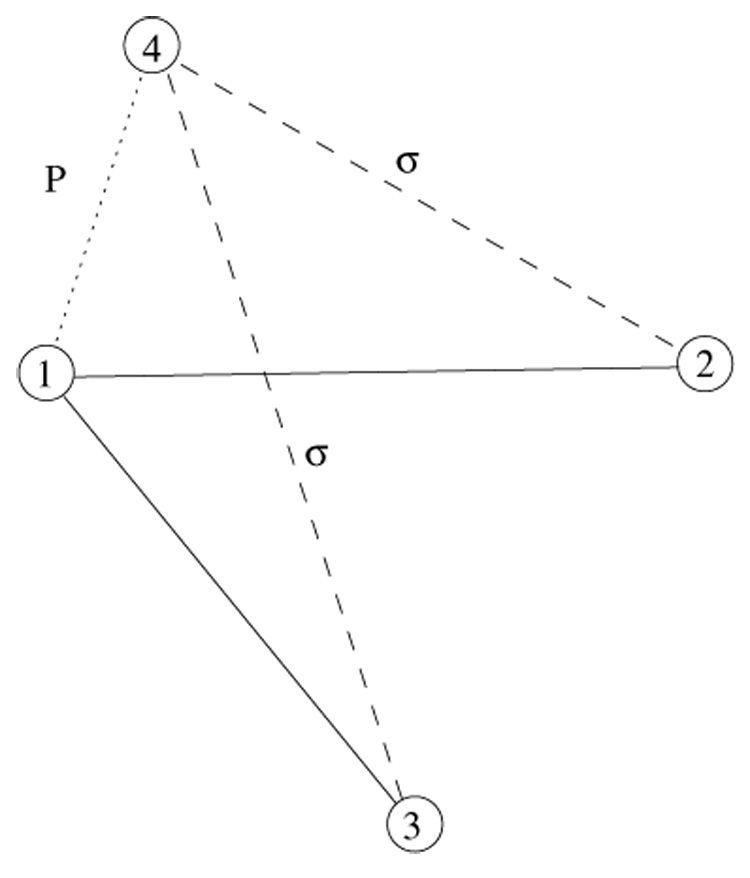
A sketch of duplication event, when a new triad is formed with a heterodimerization link. Solid lines correspond to the existing links, dotted line is a heterodimerization link, established with the probability P, and dashed lines denote the inherited with probability σ links.

Figure 2.

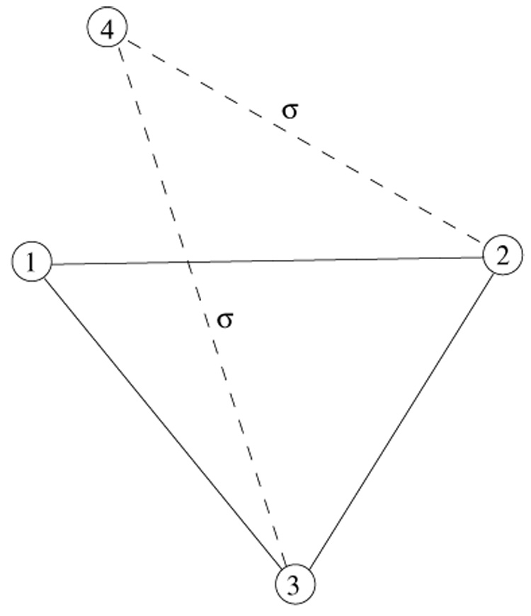
A sketch of duplication event when a new triad is formed by duplicating the existing one. Solid lines correspond to the existing links and dashed lines denote the links, each inherited with the probability σ.

In the second process (figure 2), a new triad is produced from the existing one when one of its vertices (vertex 1) is duplicated. The new triad is formed only if both links, 4-2 and 4-3 survive divergence, which happens with the probability σ². Correspondingly, a rate equation for the increase in the number of triads C₃ per duplication–divergence–heterodimerization step contains two terms,

$$\Delta C_3=\sigma P\frac{2L}{N}+{\sigma }^2\frac{3C_3}{N},$$ (1)

where L and N are the numbers of links and vertices in the network. The fraction 2L/N in the first term is an average number of links picked up for a potential triad (which is also equal to the average degree 〈d〉). The factor 3 in the second term indicates that each of the three vertices in the existing triad can be picked up as a target vertex for duplication.

Considering links as 2-cliques, the first term in equation (1) can be interpreted as describing a creation of 3-clique from a lower-order 2-clique. It is easy to see that with such an interpretation, equation (1) can be generalized to describe the evolution of population of cliques of an arbitrary order:

$$\frac{\Delta C_j}{\Delta N}=\frac{(j-1)C_{j-1}P{\sigma }^{j-2}}{\nu N}+\frac{j{C}_j{\sigma }^{j-1}}{\nu N}.$$ (2)

Here, ν ⩽ 1 is an increment in the number of vertices per duplication step. In the following, we focus on a biologically-relevant regime of 0 < σ < 1/2, where the average degree 〈d〉 is constant or almost constant [7]. In this regime ν = 2σ, and assuming the usual scaling for C_j, namely C_j ≡ Nc_j, one obtains a recurrent relation for the rescaled j-clique abundance:

$$c_j=\frac{(j-1)c_{j-1}{\sigma }^{j-3}P}{2-j{\sigma }^{j-2}}.$$ (3)

For large j, the second term in denominator becomes subdominant (jσ^j−2 ≪ 2), and therefore

$$c_j~(j-1)!{\sigma }^{(j-3)(j-2)/2}{(P/2)}^{j-2}.$$ (4)

Hence, the relative population of large cliques decays faster than exponentially. This renders large cliques highly improbable in networks of biologically relevant size of N ~ 10⁴.

To check the analytical prediction (3), and to see if the proposed duplication–divergence–heterodimerization model explains the observed population of cliques, we performed a numerical simulation. We fixed σ = 0.38 so that the average degree is equal to that of the fly dataset, where 〈d〉 ≈ 5.9 for N = 6954 proteins [22]. We selected P = 0.03, so that the number of triads in the simulated network is also similar to that in the fly dataset and count the number of 4- and 5-cliques in the resulting network. The theoretical predictions for C_j were computed from recurrence (3) by taking into account that c₂ ≡ 〈d〉/2. Results of simulations $C_j^s$ averaged over 2000 network realizations, the theoretical predictions $C_j^{th}$, and empirical results for the clique abundances in the fly dataset $C_j^{\mathit{\text{fly}}}$ are shown in table 1. The agreement between the experimental dataset, simulations, and equation (3) is surprisingly good, especially given the fact that for σ = 0.38, 〈d〉 = constant only approximately [7].

Table 1.

Number of j-cliques in networks with N = 6954 vertices and L = 20435 links for, $C_j^{\mathit{\text{fly}}}$—fruitfly protein–protein-binding network, $C_j^s$—simulations with σ = 0.38 and P = 0.03, and $C_j^{th}$—equation (3) prediction for the same σ and P.

j	$C_j^{\text{fly}}$	$C_j^s$	$C_j^{th}$
3	1405	1371 ± 9	1416
4	35	33 ± 1	34
5	1	0.37 ± 0.04	0.34
6	0	0.0025 ± 0.0016	0.0014

3. Arbitrary divergence

In this section, we extend the results obtained in [7] and above for the completely asymmetric divergence to the general situation. The arbitrary divergence model is defined as follows:

1. Duplication. A randomly chosen target node is duplicated, that is, its replica is introduced and connected to all neighbours of the target node.

2. Divergence. Each link emanating from either the target or the replica node is independently removed with probability 1 – σ₁ and 1 – σ2, respectively. This mimics disappearance of links during divergence from initially indistinguishable target and replica nodes. Vertices that have lost all their links during this process (this may include both the target and the replica vertices as well as their neighbours) are discarded.

The completely asymmetric version considered in [7] corresponds to σ₁ = 1, σ₂ = σ; the symmetric version (σ₁ = σ₂) of our model slightly differs from a model investigated by Vázquez and co-workers [4].

The existing links were never lost in completely asymmetric divergence, and the network remained connected if it were initially connected. When σ₁ < 1, however, the network does lose old links, which may result in splitting it into disconnected components which would never reconnect.

We ignore heterodimerization in the following discussion of the network growth and degree distribution (section 3.1 and section 3.2) since in the biologically interesting regime P ≪ σ₁, σ₂, and the total fraction of heterodimerization links is negligible. Naturally, in describing the clique generation (section 3.3) we will of course add heterodimerization.

3.1. Growth law

As in [7], an increment in the number of links L during a duplication step is

$$\frac{\Delta L}{\Delta N}=\frac{2L({\sigma }_1+{\sigma }_2-1)}{\nu N},$$ (5)

where N is the number of vertices, 2L/N ≡ 〈d〉 is the average number of neighbours or the average degree, and 0 < ν ⩽ 1 is an increment in the number of vertices per step. Assuming that for a large network, ν does not depend on the network size N, we obtain

$$L(N)~N^{2({\sigma }_1+{\sigma }_2-1)/\nu }.$$ (6)

There are three distinct regimes of network growth:

1. Since at a duplication step the number of vertices cannot increase by more than one, ν ⩽ 1, and therefore, for σ₁ + σ₂ > 3/2 the growth of L(N) is superliniear. The average degree grows as a power-law of a network size, and for sufficiently large networks the probability to eliminate all the links and therefore, not to add a vertex at a duplication step becomes negligible. Hence for large networks ν → 1 and

   $$L~N^{2({\sigma }_1+{\sigma }_2-1)}.$$ (7)

2. For σ₁ + σ₂ ⩽ 3/4 and ${\sigma }_1>{\sigma }_1^{*},{\sigma }_2>{\sigma }_2^{*}$ (where the lower bounds ${\sigma }_i^{*}$ will be determined below), we observe that the average degree increases logarithmically and L ~ N ln N.

3. Since only linked vertices are counted, the average degree cannot decrease below unity. Hence, even for small link retention probability, 1 < σ₁ + σ₂, and ${\sigma }_1<{\sigma }_1^{*},{\sigma }_2<{\sigma }_2^{*}$, the growth of L is linear, L ~ N and the average degree saturates to a constant.

When σ₁ + σ₂ < 1, the network loses links faster than it gains new links and quickly disappears (since vertices that lost all links are discarded).

3.2. Degree distribution

The degree distribution N_k evolves according to the following rate equation (see [7] for details of a similar derivation)

$$\nu \frac{\Delta N_k}{\Delta N}=\frac{N_{k/{\sigma }_1}}{N{\sigma }_1}+\frac{N_{k/{\sigma }_2}}{N{\sigma }_2}-\frac{N_k}{N}+({\sigma }_1+{\sigma }_2-1)\left[\frac{(k-1)N_{k-1}-k{N}_k}{N}\right].$$ (8)

Here, the first three terms describe the gain of two new degrees of the duplicated vertices and the loss of an old degree of the target vertex, while the fourth term accounts for a change in the number of degrees of a neighbour of a target vertex. Substituting N_k ∝ Nk^−γ and using ν = 2(σ₁ + σ₂ − 1)(which follows from (5)), we obtain

$${\sigma }_1^{\gamma -1}+{\sigma }_2^{\gamma -1}+({\sigma }_1+{\sigma }_2-1)(\gamma -1)+1-2({\sigma }_1+{\sigma }_2)=0.$$ (9)

This equation has a trivial solution γ′ = 2 and a non-trivial σ-dependent solution γ(σ₁, σ₂). These two solutions coincide along the line $({\sigma }_1^{*},{\sigma }_2^{*})$ in the (σ₁, σ₂) plane defined by the equation

$${\sigma }_1^{*}(\text{ln}{\sigma }_1^{*}+1)+{\sigma }_2^{*}(\text{ln}{\sigma }_2^{*}+1)=1.$$ (10)

An important example is the symmetric case, ${\sigma }_1^{*}={\sigma }_2^{*}\approx 0.72985$ in the completely asymmetric case, σ₁ ≡ 1 and ${\sigma }_2^{*}=1/e\approx 0.36879$.

A phase diagram in the (σ₁, σ₂) space that represents various regimes of the network growth is shown in figure 5. The exponent γ is plotted in figure 6 for the symmetric case σ₁ = σ₂ = σ. The measured in simulation degree distribution for 1/2 < σ < σ* does not contradict the predicted power-law asymptotics, figure 7.Yet the true asymptotic regime is reached for far larger networks than the biological protein–protein graphs [7], and the full functional form of the degree distribution or even the corrections to scaling remain unknown.

Figure 5.

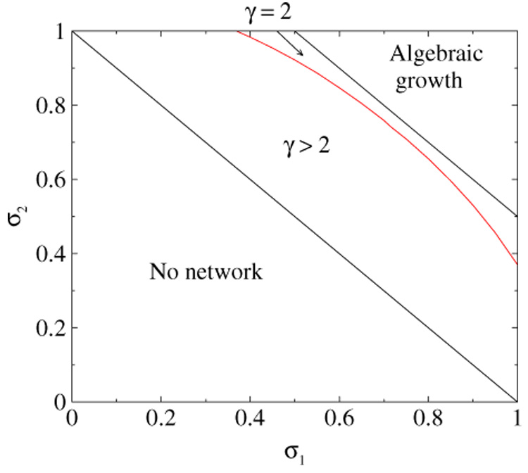
The curved line (10) and the straight line σ₁ + σ₂ = 3/2 separate qualitatively different network regimes. In the region denoted as ‘algebraic growth’ the average degree increases as 〈d〉 ~ N^{2(σ₁+σ₂−3/2)} and the degree distribution has a scaling form shown in figure 4.

Figure 6.

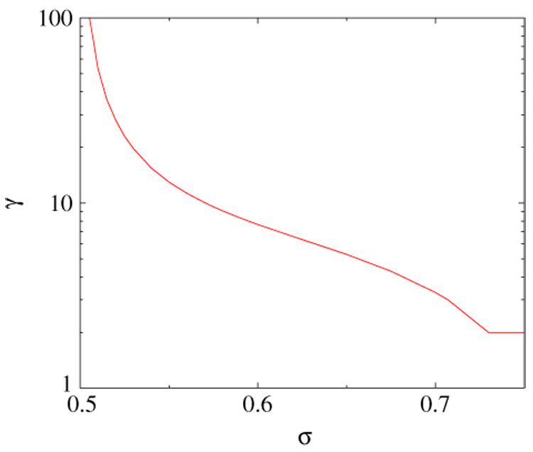
The degree distribution exponent γ(σ) for the symmetric divergence from equation (9), γ ≈ 1/(2σ − 1) for σ → 1/2 + 0.

Figure 7.

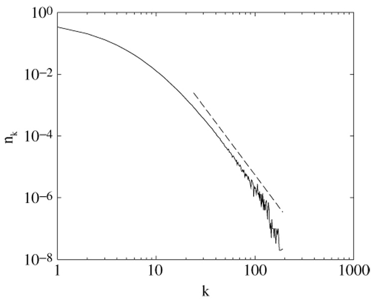
The degree distribution n_k for symmetric divergence, σ₁ = σ₂ = 0.675. A dashed line is the predicted power-law asymptotics with the exponent γ(0.675) ≈ 4.3.

A summary of results for the arbitrary symmetric duplication–divergence is presented in table 2.

Table 2.

The behaviour of the duplication–divergence network of arbitrary symmetry for different values of probabilities to preserve a link σ₁ and σ₂. Here, L(N) is the average number of links for a given number of nodes N, n_k the average fraction of nodes of degree k. ${\sigma }_i^{*}$, i = 1, 2 are the solutions of equation (5), γ(σ₁, σ₂) is given by equation (9).

σ	Self-averaging	L(N)	nk
σ1 = σ2 = 1	No	N(N + 1)/6	2(N − k)/[N(N − 1)]
3/2 < σ1 + σ2 < 1	No	~N2(σ1+σ2−1)	~N3−2σ1−2σ2F(k/N2σ1+2σ2−3)
σ1 + σ2 < 3/2, σi > ${\sigma }_i^{*}$, i = 1, 2	Yes	~N ln N	probably ~k−2
1/2 < σ1 + σ2, σi < ${\sigma }_i^{*}$, i = 1, 2	Yes	~N	~k−γ(σ1,σ2)

3.3. Cliques

Similarly to the completely asymmetric divergence considered above, to generate cliques one must add heterodimerization to the pure duplication and divergence. Hence, we assume that a target node and a replica node are linked with probability P.

A generalization of equation (2) reads

$$\frac{\Delta C_j}{\Delta N}=\frac{(j-1)C_{j-1}P{({\sigma }_1{\sigma }_2)}^{j-2}}{\nu N}+\frac{j{C}_j{({\sigma }_1{\sigma }_2)}^{j-1}}{\nu N}-\frac{j{C}_j(1-{\sigma }_1^{j-1})(1-{\sigma }_2^{j-1})}{\nu N}.$$ (11)

Since the creation of a new clique requires that all links emanating both from the target and replica vertices survive divergence, in the first two terms σ is replaced by σ₁σ₂. The third term accounts for the loss of j-cliques due to disappearance of at least one link both from the target and replica nodes. Following the procedure for the asymmetric case and taking into account that in the scaling regime where 1 < σ₁ + σ₂ < 3/2 an increment in the number of vertices per step is ν = 2(σ₁ + σ₂ − 1), we obtain the following recurrence analogous to equation (3):

$$c_j=\frac{(j-1)c_{j-1}{({\sigma }_1{\sigma }_2)}^{j-2}P}{2({\sigma }_1+{\sigma }_2-1)-j({\sigma }_1^{j-1}+{\sigma }_2^{j-1}-1)}.$$ (12)

We checked this prediction, in the symmetric case (σ₁ = σ₂ = σ) using the fly dataset [22] for reference. The correct average degree and number of triads are obtained when σ ≈ 0.725 and P ≈ 0.0475. The experimental, simulation, and theoretical results, shown in table 3, are again in very good agreement.

Table 3.

Number of j-cliques in networks with N = 6954 vertices and L = 20435 links for $C_j^{\mathit{\text{fly}}}$—fruitfly protein–protein-binding network, $C_j^s$—simulation of symmetric divergence with σ₁ = σ₂ = 0.725 and P = 0.0475, and $C_j^{th}$—equation (12) prediction for the same σ and P. Simulation results are averaged over 2000 network realizations.

j	$C_j^{\text{fly}}$	$C_j^s$	$C_j^{th}$
3	1405	1353 ± 9	1377
4	35	28 ± 1	28
5	1	0.24 ± 0.03	0.24
6	0	0.0025 ± 0.0016	0.0011

3.4. Integrity of the network

For symmetric divergence, we have measured the number of components and the size of the largest component for the networks grown with various σ₁ = σ₂ = σ. The results for the networks of the size of fruitfly dataset, N= 6954, are presented in table 4.

Table 4.

Number of components n_c and the number of vertices in the largest component normalized by the network size, N_L/N, in the duplication–symmetric-divergence networks for various σ₁ = σ₂ = σ. All networks are grown to the fly dataset size, N = 6954; the results are averaged over 1000 realizations.

σ	nc	NL/N
0.8	1.1 ± 0.01	99 ± 0.2%
0.725	8.4 ± 0.2	92 ± 0.4%
0.65	232 ± 1	33 ± 1%
0.6	835 ± 1.4	2.7 ± 0.03%

For 1/2 < σ ≲ σ* we have found that the grown network contains many fairly small components, while, for σ* < σ there is usually one or a few large components and several small ones. Intuitively, it is clear that if the average degree grows, even slowly, the probability to split the network into many parts becomes small.

A theoretical prediction for the size of the giant component exists only for the Erdős–Rényi random graph [24]: when the average degree scales logarithmically with the number of vertices, i.e., 〈d〉 = p ln N, the total number of vertices that do not belong to the giant component scales as N^1−p for p < 1, while for p > 1 the giant component engulfs the entire system. It turns out that for the same number of vertices and links, the completely random linking of the Erdős–Rényi graph keeps more vertices in a giant component than the corresponding duplication–symmetric-divergence network. Indeed, for the parameters corresponding to the fly dataset, σ₁ = σ₂ = 0.725, N = 6954, 〈d〉 ≈ 5.9, and accordingly p= 0.667. The number of vertices not belonging to the giant component is 6954 × 0.08 ≈ 556 (see table 4), while the random graph with the same number of vertices and links has about 69540^0.333 ≈ 19 vertices disconnected from the giant component. This happens mainly because in our duplication–divergence growth model, once a component splits from the giant component, it never reconnects. If such separation happens at an early stage of the network growth, the separated component may grow to a significant size, thus leaving many vertices outside of the giant component. On contrary, at each step of the Erdős–Rényi growth, any two components can be united with a random link. This makes the co-existence of two or more large components very improbable.

4. Discussion and conclusion

In the previous sections, we obtained the following results for the clique abundance and growth laws of the duplication–divergence–heterodimerization networks:

• For the duplication–divergence network growth model with completely asymmetric divergence [7], complimented with heterodimerization links between duplicates, we computed the clique population distribution and found that it agrees well with empirical data.

• Generalizing results obtained for the completely asymmetric divergence, we demonstrated that similar regimes, such as presence and lack of self-averaging, growth and saturation of the average degree, scaling and fat-tail in the degree distribution, exist in the general duplication–divergence case. We also computed the clique population distribution for the arbitrary divergence scenario.

The heterodimerization links are not taken into account in our description of the network growth and degree distribution. Despite their crucial role in the network topology and clique formation, they constitute only about 1% of all links and do not contribute significantly to the degrees of most of the vertices. For link inheritance and heterodimerization probabilities σ and P, corresponding to the fly dataset, the resulting number of heterodimeric links in a network of the size of the fly dataset is L_hd ≈ PN/(2 σ) ≈ 270. This is somewhat higher than the observed number of links between the pairs of recently duplicated (paralogous) proteins $L_{hd}^{\mathit{\text{fly}}}=142$ [17]. The main reason for this discrepancy is that in our simulation, all heterodimeric links are counted, while in the real protein network one can reliably identify only the pairs of recently duplicated proteins. Another reason may be in the ‘mean-field’ character of our model: while we chose the target–replica pairs for heterodimerization at random, in reality, a propensity for dimerization is often inherited. Thus, in real networks a community of descendants of a dimer may have a higher than average concentration of heterodimers. Such local enhancement of heterodimerization can produce more cliques per heterodimer link than in our ‘uniform’ heterodimerization case.

In the case of not completely asymmetric divergence, when links can disappear both from the target and replica nodes, a network may fragment into several components. Yet the biological protein networks are believed to be connected to ensure their functionality. Hence, during in vivo divergence, the steps that lead to breaking the network into isolated components are excluded due to evolutionary pressure. Our probabilistic network growth model does not take any evolutionary pressure into account. However, since for sufficiently high link retention probabilities the resulting network consists of one or very few large components, the number of link eliminations that have to be evolutionary overridden is small. Hence, most of the properties of the probabilistically grown graphs should be similar to those of the realistic evolutionary single-component networks. As the link inheritance probabilities σ_i decrease and the number of network components grow, the number of link removal steps that have to be evolutionary overridden becomes large. Consequently, the probabilistic multi-component network becomes less similar to the real single-components one.

As we mentioned in the section 2, an example of the fly dataset was selected as being the most non-subjective one. Yet, we believe that the proposed network growth mechanism is biologically justified and with a proper choice of parameters, it should correctly predict clique abundance in any protein–protein network. However, other currently known protein–protein networks, such as for yeast, worm, and human, do contain parts of data that are results of the ‘matrix’ recording of the experimental data from the immunoprecipitation experiments. These datasets contain a higher number of large cliques, which can be attributed to this data interpretation and in reality are tightly, but not completely, linked protein complexes. In principle, the clique population distribution derived here can be used to verify and filter the experimental datasets, revealing the erroneously recordered large cliques.

In a recent publication, Middendorf et al [25] compared topological properties of the fly dataset to those of the networks grown by several mechanisms such as different versions of duplication–mutation model and preferential attachment. It was found that the abundance of many types of small subgraphs, including, but by far not limited to cliques, ‘duplication–mutation–complementation’ networks provide the best fit to the fly dataset. The duplication–mutation–complementation network growth model is very close to the duplication–divergence–heterodimerization model studies here. ‘Conjoining’ in [25] is equivalent to heterodimerization in our model, the only difference between the two models is in the way the links are deleted during divergence (or mutation): unlike our model, in [25] each neighbour remains connected to at least one of the two duplicates. Thus, our works confirm the conclusions made in [25] that the majority of considered properties of protein–protein networks are very well described by the duplication–divergence–heterodimerization model.

And finally, a few words on the importance of heterodimerization links in clique formation. An alternative to the heterodimerization way of connecting paralogs is to link them randomly by ‘mutation’links. In this case, the probability to establish a heterodimeric link P has to be replaced by a probability that a mutation link, emanating from a target node, selects the replica node out of N network nodes. This probability is equal to M/N, where M is the number of mutation links established at each duplication step. In the example of the fruitfly dataset, where P = 0.03 and N = 6954, one needs M = NP = 209 random links at each step to form the correct number of triads and higher cliques. Obviously, the mutation scenario which requires so many additional links is completely ruled out due to, for example, the average degree constraint.

Figure 3.

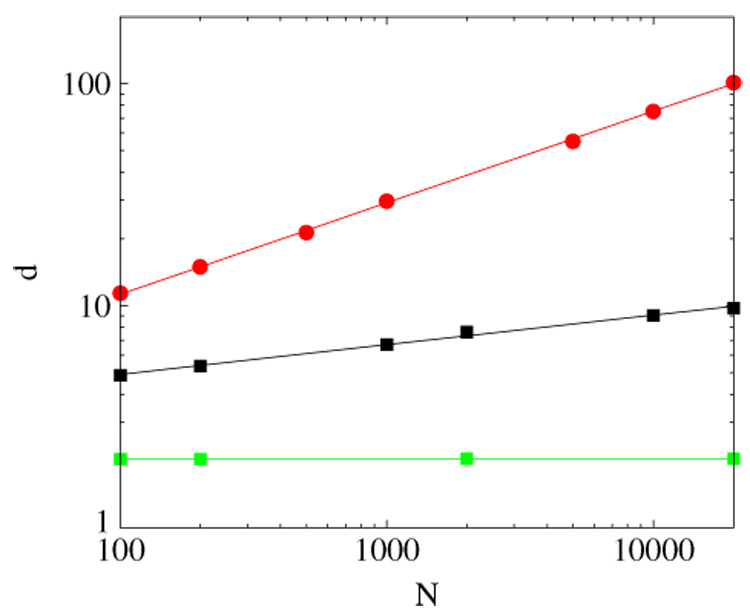
The average node degree 〈d〉 versus N for (bottom to top) the completely symmetric network growth, σ₁ = σ₂ = 0.6, 0.75, 0.85. Solid lines are the corresponding best fits, 〈d〉 = constant for σ₁ = σ₂ = 0.6, 〈d〉 ~ N^0.14 or 〈d〉 ~ ln N for σ₁ = σ₂ = 3/4, and 〈d〉 ~ N^0.14 for σ₁ = σ₂ = 0.85 (〈d〉 ~ N^0.4 follows from equation (7)).The results are averaged over 100 network realizations.

Figure 4.

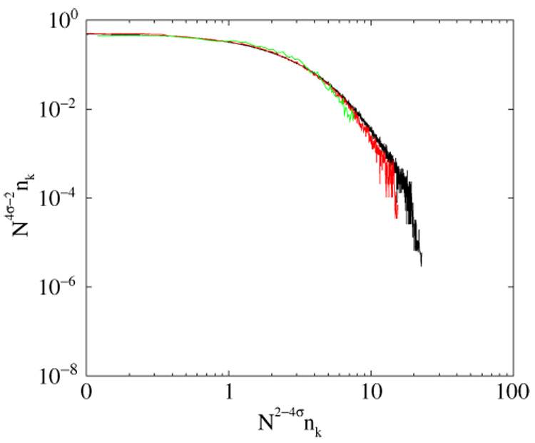
Scaling of the degree distribution in the networks of N = 200, N = 2000, and N= 20 000 nodes with σ₁ = σ₂ = 0.85.

References

- 1.Ohno S. Evolution by Gene Duplication. New York: Springer; 1970. [Google Scholar]
- 2.Taylor JS, Raes J. Annu. Rev. Genet. 2004;9:615–643. doi: 10.1146/annurev.genet.38.072902.092831. [DOI] [PubMed] [Google Scholar]
- 3.Solé RV, Pastor-Satorras R, Smith ED, Kepler T. Adv. Complex Syst. 2002;5:43. [Google Scholar]
- 4.Vázquez A, Flammini A, Maritan A, Vespignani A. ComPlexUs. 2003;1:38–44. [Google Scholar]
- 5.Kim J, Krapivsky PL, Kahng B, Redner S. Phys. Rev. E. 2002;66:055101. doi: 10.1103/PhysRevE.66.055101. [DOI] [PubMed] [Google Scholar]
- 6.Dokholyan NV, Shakhnovich B, Shakhnovich EI. Proc. Natl Acad. Sci. USA. 2002;99:14132–14136. doi: 10.1073/pnas.202497999. [DOI] [PMC free article] [PubMed] [Google Scholar]
- 7.Ispolatov I, Krapivsky PL, Yuryev A. 2004 Preprint q-bio.MN/0411052. [Google Scholar]
- 8.Milo R, Itzkovitz S, Kashtan N, Levitt R, Shen-Orr S, Ayzenshtat I, Sheffer M, Alon U. Science. 2004;303:1538. doi: 10.1126/science.1089167. [DOI] [PubMed] [Google Scholar]
- 9.Milo R, Shen-Orr S, Itzkovitz S, Kashtan N, Chklovskii D, Alon U. Science. 2002;298:824. doi: 10.1126/science.298.5594.824. [DOI] [PubMed] [Google Scholar]
- 10.Bianconi G, Caldarelli G, Capocci A. 2003 Preprint cond-mat/0310339. [Google Scholar]; Bianconi G, Caldarelli G, Capocci A. 2004 Preprint cond-mat/0408349. [Google Scholar]
- 11.Rozenfeld HD, Kirk JE, Bollt EM, ben-Avraham D. 2004 Preprint cond-mat/0403536. [Google Scholar]
- 12.Sergi D. 2004 Preprint cond-mat/0412472. [Google Scholar]
- 13.Collet P, Eckmann JP. J. Stat. Phys. 2002;109:923. [Google Scholar]
- 14.Vazquez A, Oliveira JG, Barabasi AL. 2005 Preprint cond-mat/0501399. [Google Scholar]
- 15.Wuchty S, Oltvai ZN, Barabasi AL. Nat Genet. 2003;35:118. doi: 10.1038/ng1242. [DOI] [PubMed] [Google Scholar]
- 16.Spirin V, Mirny LA. Proc. Natl Acad. Sci. USA. 2003;100:12123. doi: 10.1073/pnas.2032324100. [DOI] [PMC free article] [PubMed] [Google Scholar]
- 17.Ispolatov I, Yuryev A, Mazo I, Maslov S. 2005 doi: 10.1093/nar/gki678. Preprint q-bio.GN/0501004. [DOI] [PMC free article] [PubMed] [Google Scholar]
- 18.Conant GC, Wagner A. Genome Res. 2003;13:2052. doi: 10.1101/gr.1252603. [DOI] [PMC free article] [PubMed] [Google Scholar]
- 19.Kondrashov FA, Rogozin IB, Wolf YI, Koonin EV. Genome Biol. 2002;2:Res.0008. doi: 10.1186/gb-2002-3-2-research0008. [DOI] [PMC free article] [PubMed] [Google Scholar]
- 20.Grant PA, Schieltz D, Pray-Grant MG, Yates JR, III, Workman JL. Mol. Cell. 1998;6:863. doi: 10.1016/s1097-2765(00)80300-7. [DOI] [PubMed] [Google Scholar]
- 21.Bader GD, Hogue CWV. Nat. Biotech. 2002;20:991. doi: 10.1038/nbt1002-991. [DOI] [PubMed] [Google Scholar]
- 22.Giot L, et al. Science. 2003;302:1727. doi: 10.1126/science.1090289. [DOI] [PubMed] [Google Scholar]
- 23.Maslov S, Sneppen K. Science. 2002;296:910. doi: 10.1126/science.1065103. [DOI] [PubMed] [Google Scholar]
- 24.Janson S, Luczak T, Rucinski A. Random Graphs. New York: Wiley; 2000. [Google Scholar]
- 25.Middendorf M, Ziv E, Wiggins C. Proc. Natl Acad. Sci. USA. 2005;102:3192. doi: 10.1073/pnas.0409515102. [DOI] [PMC free article] [PubMed] [Google Scholar]