Image description with generalized pseudo-Zernike moments

Abstract

A new set of orthogonal moment functions for describing images is proposed. It is based on the generalized pseudo-Zernike polynomials that are orthogonal on the unit circle. The generalized pseudo-Zernike polynomials are scaled to ensure the numerical stability, and some properties are discussed. The performance of the proposed moments is analyzed in terms of image reconstruction capability and invariant character recognition accuracy. Experimental results demonstrate the superiority of generalized pseudo-Zernike moments compared with pseudo-Zernike and Chebyshev-Fourier moments in both noise-free and noisy conditions.

1. Introduction

In the past decades, various moment functions due to their abilities to represent the image features have been proposed for describing images.^1–10 In 1962, Hu² first derived a set of moment invariants, which are position, size and orientation independent. These moment invariants have been successfully used in the field of pattern recognition.^3–5 However, geometric moments are not orthogonal and as a consequence, reconstructing the image from the moments is deemed to be a difficult task. Based on the theory of orthogonal polynomials, Teague⁶ has shown that the image can be easily reconstructed from a set of orthogonal moments, such as Legendre moments and Zernike moments. Teh and Chin⁷ evaluated various types of image moments in terms of noise sensitivity, information redundancy and image description capability, they found that pseudo-Zernike moments (PZMs) have the best overall performance.

Recently, Ping et al.⁸ introduced Chebyshev-Fourier moments (CHFMs) for describing image. By analyzing the image-reconstruction error and image distortion invariance of the CHFMs, they concluded that CHFMs perform better than the orthogonal Fourier-Mellin moments (OFMMs), which was proposed by Sheng and Shen⁹ in 1994. Both CHFMs and OFMMs are orthogonal and invariant under image rotation.

In this paper, we propose a new kind of orthogonal moments, known as generalized pseudo-Zernike moments (GPZMs), for image description. The GPZMs are defined in terms of the generalized pseudo-Zernike polynomials (GPZPs) that are an expansion of the classical pseudo-Zernike polynomials. The two-dimensional (2D) GPZPs, $V_{pq}^{\alpha }(z,z^{\ast })$, are orthogonal on the unit circle with weights (1 − (zz*)^l/2)^α where α > −1 is a free parameter. The location of the zero points of real-valued radial GPZPs depends on the parameter α, so it is possible to choose appropriate values of α for different kinds of images. Experimental results demonstrate that the proposed moments perform better than the conventional PZMs and CHFMs in terms of image reconstruction capability and invariant pattern recognition accuracy in both noise-free and noisy conditions.

The paper is organized as follows. In Section 2, we first give a brief outline of PZMs. The definition of GPZPs, the corresponding weighted polynomials and the GPZMs is also presented in this section. Experimental results are provided to validate the proposed moments and the comparison analysis with previous works is given in Section 3. Section 4 concludes the paper.

2. Generalized pseudo-Zernike moments

In this section, we first give a brief outline of PZMs, they will also serve as a reference to compare the performance of GPZMs. We then present the GPZPs and establish some useful properties of them in the second subsection. The definition of GPZMs is given in the last subsection.

A. Pseudo-Zernike moments

The 2D pseudo-Zernike moment (PZMs), Z_pq, of order p with repetition q is defined using polar coordinates (r, θ) inside the unit circle as^10,

$$Z_{pq}=\frac{p+1}{\pi }\underset{0}{\overset{2\pi }{\int }}\underset{0}{\overset{1}{\int }}{V}_{pq}^{\ast }(r,\theta )f(r,\theta )\mathit{rdrd}\theta ,\mathrm{\hspace{0.17em} }\mathrm{\hspace{0.17em} }\mathrm{\hspace{0.17em} }p=0,\hspace{0.17em}1,\hspace{0.17em}2,\hspace{0.17em}\dots ,\hspace{0.17em}\infty ;0\le \mid q\mid \le p.$$ (1)

where * denotes the complex conjugate, and V_pq(r, θ) is the pseudo-Zernike polynomial given by

$$V_{pq}(r,\theta )=R_{pq}(r)exp(jq\theta )$$ (2)

Here R_pq (r) is the real-valued radial polynomial defined as

$$R_{pq}(r)=\sum _{s=0}^{p-\mid q\mid }\frac{{(-1)}^k(2p+1-s)!}{s!(p-\mid q\mid -s)!(p+\mid q\mid +1-s)!}{r}^{p-s}$$ (3)

The pseudo-Zernike polynomials satisfy the following orthogonality property

$$\underset{0}{\overset{2\pi }{\int }}\underset{0}{\overset{1}{\int }}{V}_{pq}(r,\theta )·V_{lk}^{\ast }(r,\theta )\mathit{rdrd}\theta =\frac{\pi }{(p+1)}{\delta }_{pl}{\delta }_{qk}$$ (4)

where δ_nm denotes the Kronecker symbol.

B. Generalized pseudo-Zernike polynomials

Wünsche¹¹ recently presented the notion of generalized Zernike polynomials in the mathematical domain. Enlightened by the research work of Wünsche, we introduce generalized pseudo-Zernike polynomials with the notation $V_{pq}^{\alpha }(z,z^{\ast })$ in representation by a pair of complex conjugate variables (z = x + jy = r exp(jθ) and z* = x − jy = r exp(−jθ)) and with real parameter α > −1 by the following definition

$$\begin{array}{l}{V}_{pq}^{\alpha }(z,z^{\ast })\equiv z^{(\mid q\mid +q)/2}{(z^{\ast })}^{(\mid q\mid -q)/2}{P}_{p-\mid q\mid }^{(\alpha ,2\mid q\mid +1)}(2{(z{z}^{\ast })}^{1/2}-1)\\ =z^{(p+q)/2}{(z^{\ast })}^{(p-q)/2}·\frac{{(\alpha +1)}_{p-\mid q\mid }}{(p-\mid q\mid )!}{{}_{2}F}_1(-p+\mid q\mid ,-p-\mid q\mid -1;\alpha +1;1-\frac{1}{{(z{z}^{\ast })}^{1/2}})\end{array}$$ (5)

where $P_n^{(\alpha ,\beta )}(u)$ denotes the Jacobi polynomials and ₂F₁ (a, b; c; x) is the hypergeometric function given by¹²

$${{}_{2}F}_1(a,b;c;x)=\sum _{k=0}^{\infty }\frac{{(a)}_k{(b)}_k}{{(c)}_k}\frac{x^k}{k!}$$ (6)

Here (a)_k is the Pochhammer symbol defined as

$${(a)}_k=a(a+1)(a+2)\dots (a+k-1)\hspace{0.17em}\hspace{0.17em}\hspace{0.17em}\text{with\hspace{0.17em}}(a_0)=1$$ (7)

Using Eqs. (6) and (7), we obtain the following basic representation of GPZPs

$$V_{pq}^{\alpha }(z,z^{\ast })=\frac{(p+\mid q\mid +1)!}{{(\alpha +1)}_{p+\mid q\mid +1}}\sum _{s=0}^{p-\mid q\mid }\frac{{(-1)}^s{(\alpha +1)}_{2p+1-s}}{s!(p-\mid q\mid -s)!(p+\mid q\mid +1-s)!}{z}^{(p+q-s)/2}{(z^{\ast })}^{(p-q-s)/2}$$ (8)

In polar coordinate system (r, θ), Eq. (8) can be expressed as

$$V_{pq}^{\alpha }(r,\theta )\equiv V_{pq}^{\alpha }(rexp(j\theta ),rexp(-j\theta ))=R_{pq}^{\alpha }(r)exp(jq\theta )$$ (9)

where the real-valued radial polynomials $R_{pq}^{\alpha }(r)$ are given by

$$R_{pq}^{\alpha }(r)=\frac{(p+\mid q\mid +1)!}{{(\alpha +1)}_{p+\mid q\mid +1}}\sum _{s=0}^{p-\mid q\mid }\frac{{(-1)}^s{(\alpha +1)}_{2p+1-s}}{s!(p-\mid q\mid -s)!(p+\mid q\mid +1-s)!}{r}^{p-s}$$ (10)

Comparing Eq. (3) with Eq. (10), it is obvious that

$$R_{pq}(r)=R_{pq}^0(r)=r^{\mid q\mid }{P}_{p-\mid q\mid }^{(0,2\mid q\mid +1)}(2r-1)$$ (11)

Eq. (11) shows that the conventional pseudo-Zernike polynomials are a particular case of GPZPs with α = 0.

We now give some useful properties of radial polynomials $R_{pq}^{\alpha }(r)$.

a. Recurrence relations

The recurrence relations can be effectively used to compute the polynomial values. For radial polynomials given by Eq. (10), we derive the following three-term recurrence relations

$$R_{pq}^{\alpha }(r)=(M_{1}r+M_2)R_{p-1,q}^{\alpha }(r)+M_3{R}_{p-2,q}^{\alpha }(r),\mathrm{\hspace{0.17em} }\mathrm{\hspace{0.17em} }\mathrm{\hspace{0.17em} }\text{for\hspace{0.17em}}p-q\ge 2$$ (12)

where

$$M_1=\frac{(2p+1+\alpha )(2p+\alpha )}{(p+q+1+\alpha )(p-q)}$$ (13)

$$M_2=-\frac{(p+q+1)(\alpha +2p)}{p+q+\alpha +1}+M_1\frac{(p+q)(p-q-1)}{(2p-1+\alpha )}$$ (14)

$$\begin{array}{l}{M}_3=\frac{(p+q)(p+q+1)(2p-2+\alpha )(2p-1+\alpha )}{2(p+q+\alpha +1)(p+q+\alpha )}+M_2\frac{(p+q)(2p-2+\alpha )}{p+q+\alpha }\\ -M_1\frac{(p+q)(p+q-1)(p-q-2)}{2(p+q+\alpha )}\end{array}$$ (15)

For the cases where p = q or p = q+ 1, we have

$$R_{qq}^{\alpha }(r)=r^q$$ (16)

$$R_{q+1,q}^{\alpha }(r)=(\alpha +3+2q)r^{q+1}-2(q+1)r^q$$ (17)

Note that the real-valued radial polynomials $R_{pq}^{\alpha }(r)$ satisfy the symmetry property about the index q, i.e., $R_{pq}^{\alpha }(r)=R_{p,-q}^{\alpha }(r)$, so that only the case where q ≥ 0 needs to be considered.

The use of recurrence relations does not need to compute the factorial function involved in the definition of radial polynomials given by Eq. (10), thus decreasing the computational complexity and avoiding large variation in the dynamic range of polynomial values for higher order of p.

b. Orthogonality

The radial polynomials $R_{pq}^{\alpha }(r)$ satisfy the following orthogonality over the unit circle

$$\underset{0}{\overset{1}{\int }}{R}_{pq}^{\alpha }(r)R_{lq}^{\alpha }(r){(1-r)}^{\alpha }\mathit{rdr}=\frac{{(p-\mid q\mid +1)}_{2\mid q\mid +1}}{(2p+\alpha +2){(\alpha +1+p-\mid q\mid )}_{2\mid q\mid +1}}{\delta }_{pl}$$ (18)

Eq. (18) leads to the following orthogonality of the GPZPs

$$\underset{0}{\overset{1}{\int }}\underset{0}{\overset{2\pi }{\int }}{V}_{pq}^{\alpha }(r,\theta ){\left[V_{mn}^{\alpha }(r,\theta )\right]}^{\ast }{(1-r)}^{\alpha }\mathit{rdrd}\theta =\frac{2\pi {(p-\mid q\mid +1)}_{2\mid q\mid +1}}{(2p+\alpha +2){(\alpha +1+p-\mid q\mid )}_{2\mid q\mid +1}}{\delta }_{pm}{\delta }_{qn}$$ (19)

The above equation shows that (1 − r)^α is the weight function of the orthogonal relation on the unit circle, the integrals with such weight functions over polynomials within the unit circle converge in usual sense only for α > −1.

A usual way to avoid the numerical fluctuation in moment computation is by means of normalization by the norm. According to Eq. (18), we define the normalized radial polynomials as follows

$${\stackrel{\sim }{R}}_{pq}^{\alpha }(r)=R_{pq}^{\alpha }(r)\sqrt{\frac{(2p+\alpha +2){(\alpha +1+p-\mid q\mid )}_{2\mid q\mid +1}}{2\pi {(p-\mid q\mid +1)}_{2\mid q\mid +1}}}$$ (20)

Fig. 1 shows the plots of ${\stackrel{\sim }{R}}_{pq}^{\alpha }(r)$ with q = 10 and p varying from 10 to 14 for α being 0, 1 and 2, respectively. It can be observed that the set of radial polynomials ${\stackrel{\sim }{R}}_{pq}^{\alpha }(r)$ is not suitable for defining moments because the range of values of the polynomials expands rapidly with a slight increase of the order. This may cause some numerical problems in the computation of moments, and therefore affects the extracted features from moments. To remedy this problem, we define the weighted generalized pseudo-Zernike radial polynomials by further introducing the square root of the weight as a scaling factor as

Fig. 1. The plots of normalized radial polynomials ${\overline{R}}_{pq}^{\alpha }(r)$.

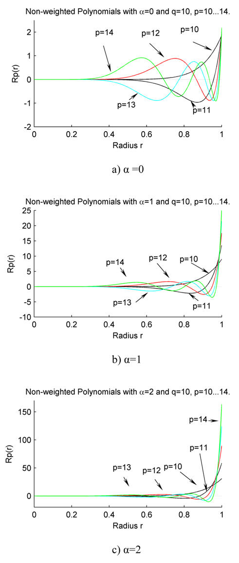
Fig. 1. a) α = 0;

Fig. 1. b) α = 1;

Fig. 1. c) α = 2.

$${\overline{R}}_{pq}^{\alpha }(r)=R_{pq}^{\alpha }(r)\sqrt{\frac{(2p+\alpha +2){(\alpha +1+p-\mid q\mid )}_{2\mid q\mid +1}}{2\pi {(p-\mid q\mid +1)}_{2\mid q\mid +1}}}{(1-r)}^{\alpha /2}$$ (21)

Fig. 2 shows the plots of weighted radial polynomials ${\overline{R}}_{pq}^{\alpha }(r)$ for some given orders with different values of α. It can be seen that the values of the functions for various orders are nearly the same. This property is good for describing an image because there are no dominant orders in the set of functions ${\overline{V}}_{pq}^{\alpha }(r,\theta )$ that will be defined below, therefore, each order of the proposed moments makes an independent contribution to the reconstruction of the image. Table 1 shows the zero point values of some weighted polynomials. It can be seen that the first zero point is shifted to small value of r as α increases. Moreover, the distribution of zero points for α between 10 and 30 is more uniform than α = 0. These properties could be useful for image description and pattern recognition tasks.

Fig. 2. The plots of weighted radial polynomials ${\overline{R}}_{pq}^{\alpha }(r)$ and their zero distributions with different values of α.

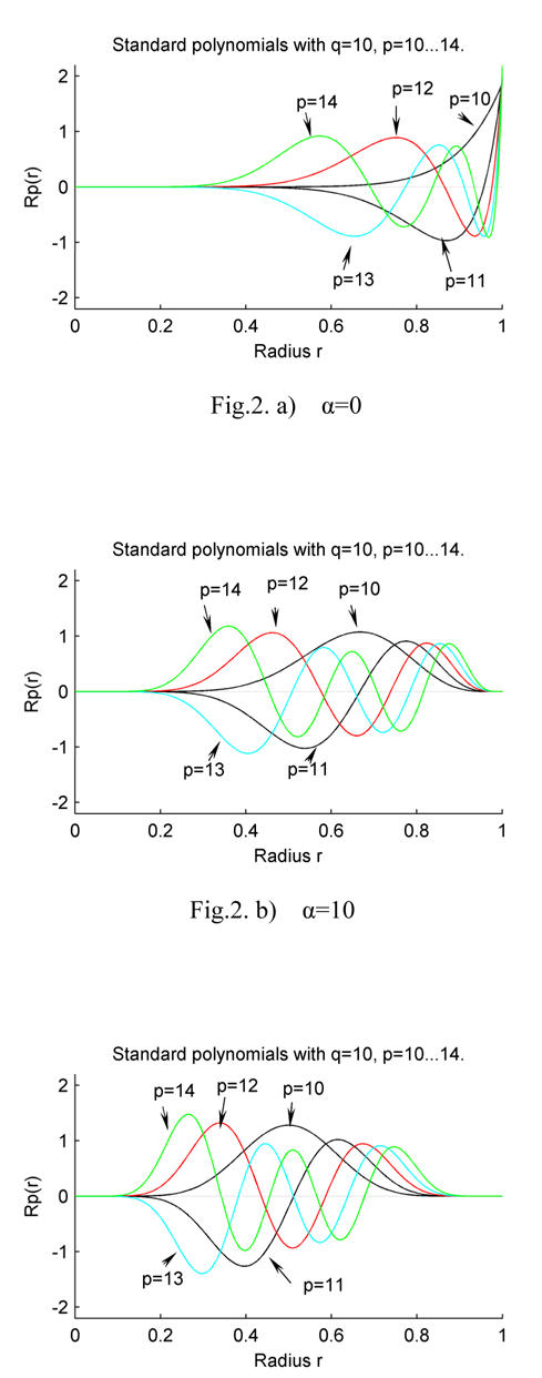
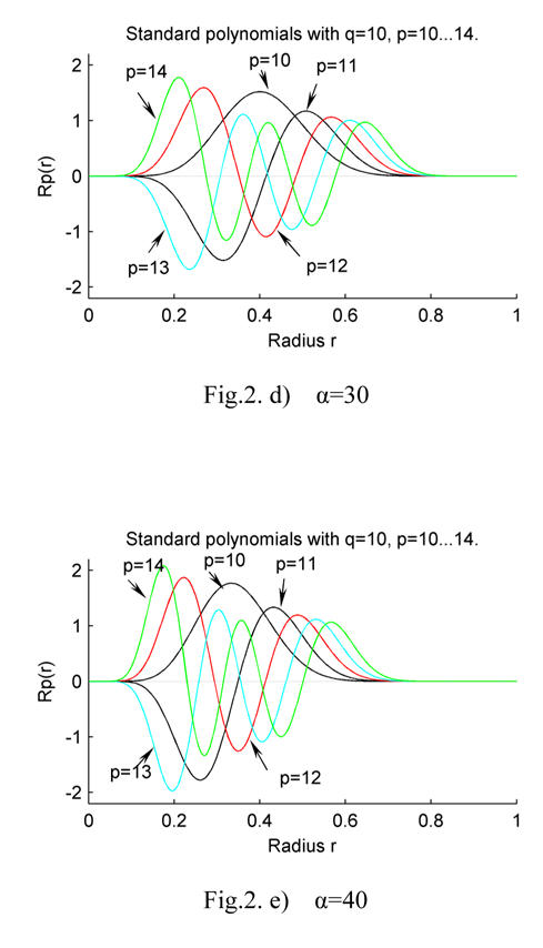
Fig. 2. a) α = 0;

Fig. 2. b) α = 10;

Fig. 2. c) α = 20;

Fig. 2. d) α = 30;

Fig. 2. e) α = 40.

Table 1.

Comparison of positions of the radial real-valued GPZP zeros with different α

The value of p (q = 10)	α=0	α =10	α =20	α =30	α =40
10	-	-	-	-	-
11	0.956563	0.666563	0.511562	0.415312	0.349063
12	0.864688	0.575938	0.435937	0.350937	0.294063
	0.975313	0.738438	0.586562	0.485312	0.413438
13	0.772813	0.508125	0.382812	0.307813	0.257188
	0.910313	0.654375	0.510937	0.419063	0.355312
	0.983438	0.783438	0.638125	0.53625	0.461875
14	0.690313	0.45375	0.341562	0.274688	0.229688
	0.836563	0.587813	0.455937	0.372188	0.315000
	0.93375	0.706563	0.565313	0.470625	0.402813
	0.987188	0.815625	0.677813	0.577187	0.501563

Let

$${\overline{V}}_{pq}^{\alpha }(r,\theta )={\overline{R}}_{pq}^{\alpha }(r)exp(jq\theta )$$ (22)

we have

$$\underset{0}{\overset{2\pi }{\int }}\underset{0}{\overset{1}{\int }}{\overline{V}}_{pq}^{\alpha }(r,\theta ){[{\overline{V}}_{nm}^{\alpha }(r,\theta )]}^{\ast }\mathit{rdrd}\theta ={\delta }_{pn}{\delta }_{qm}$$ (23)

C. Generalized pseudo-Zernike moments

The 2D GPZMs ${\overline{Z}}_{pq}^{\alpha }$ of order p with repetition q are defined as

$${\overline{Z}}_{pq}^{\alpha }=\underset{0}{\overset{2\pi }{\int }}\underset{0}{\overset{1}{\int }}{[{\overline{V}}_{pq}^{\alpha }(r,\theta )]}^{\ast }f(r,\theta )\mathit{rdrd}\theta$$ (24)

The corresponding inverse transform is

$$f(r,\theta )=\sum _{p=0}^{\infty }\sum _q{\overline{Z}}_{pq}^{\alpha }{\overline{V}}_{pq}^{\alpha }(r,\theta )$$ (25)

If only the moments of order up to M are available, Eq. (25) is usually approximated by

$$\stackrel{\sim }{f}(r,\theta )=\sum _{p=0}^M\left\{{\overline{Z}}_{p0}^{{\alpha }^{(c)}}{\overline{R}}_{p0}^{\alpha }(r)+2\sum _{q>0}[{\overline{Z}}_{pq}^{{\alpha }^{(c)}}cos(q\theta )+\sum _{q>0}{\overline{Z}}_{pq}^{{\alpha }^{(s)}}sin(q\theta )]{\overline{R}}_{pq}^{\alpha }(r)\right\}$$ (26)

where

$$\begin{array}{l}{\overline{Z}}_{pq}^{{\alpha }^{(c)}}=\underset{0}{\overset{2\pi }{\int }}\underset{0}{\overset{1}{\int }}{\overline{R}}_{pq}^{\alpha }(r)f(r,\theta )cos(q\theta )·\mathit{rdrd}\theta ,\hfill \\ {\overline{Z}}_{pq}^{{\alpha }^{(s)}}=-\underset{0}{\overset{2\pi }{\int }}\underset{0}{\overset{1}{\int }}{\overline{R}}_{pq}^{\alpha }(r)f(r,\theta )sin(q\theta )·\mathit{rdrd}\theta \hfill \end{array}\mathrm{\hspace{0.17em} }\mathrm{\hspace{0.17em} }\mathrm{\hspace{0.17em} }q\ge 0,$$ (27)

For a digital image of size N × N, Eq. (24) is approximated by^13,14

$${\overline{Z}}_{pq}^{\alpha }=\frac{2}{{(N-1)}^2}\sum _{s=0}^{N-1}\sum _{t=0}^{N-1}{\overline{R}}_{pq}^{\alpha }(r_{st})exp(-jq{\theta }_{st})f(s,t)$$ (28)

where the image coordinate transformation to the interior of the unit circle is given by

$$r_{st}=\sqrt{{(c_{1}s+c_2)}^2+{(c_{1}t+c_2)}^2},{\theta }_{st}={tan}^{-1}\left(\frac{c_{1}t+c_2}{c_{1}s+c_2}\right),\hspace{0.17em}{c}_1=\frac{\sqrt{2}}{N-1},\hspace{0.17em}{c}_2=-\frac{1}{\sqrt{2}}$$ (29)

3. Experimental results

In this section, we evaluate the performance of the proposed moments. Firstly, we address the problem of reconstruction capability of the proposed method, and compare it with that of CHFM. The recognition accuracy of GPZMs is then tested and compared with CHFM.

A. Image reconstruction

In this subsection, the image representation capability of GPZMs is first tested using a set of binary images. The GPZMs are computed with Eq. (28) and the image representation power is verified by reconstructing the image using the inverse transform (26). An objective measure is used to quantify the error between the original image f(x, y) and the reconstructed image f̂(x, y), and it is defined as

$$\epsilon =\sum _{x=0}^{N-1}\sum _{y=0}^{N-1}\mid f(x,y)-T(\widehat{f}(x,y))\mid$$ (30)

where T(.) is the threshold operator

$$T(u)=\{\begin{array}{ll}1\hfill & u\ge 0.5\hfill \\ 0\hfill & u<0.5\hfill \end{array}$$ (31)

The uppercase English letter “E” of size 31 × 31 and a Chinese character of size 63 × 63 are first used as test images. Tables 2 and 3 show the reconstructed images as well as the relative errors for GPZMs with α = 0, 4, 8, 12, and CHFMs respectively. Other values of α have also been tested in this experiment, the detail reconstruction errors for GPZMs with α = 0, 10, 20, and CHFMs are shown in Figs. 3 and 4, respectively. As can be seen from the figures, the reconstruction error decreases for the same order of moment when the value of α increases. It can also be observed that the GPZMs (except for α = 0) perform better than the CHFMs, and the difference becomes more important when higher order of moments is used.

Table 2.

Image Reconstruction of the letter “E” of size 31×31 without noises

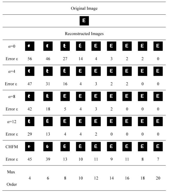Table 3.

Image Reconstruction of a Chinese character of size 63 × 63 without noise

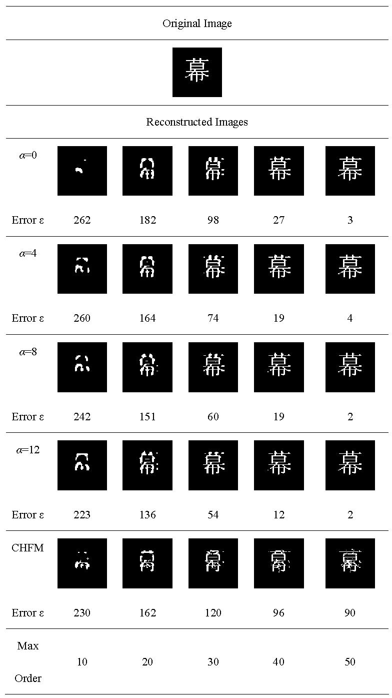Fig. 3.

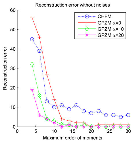
Plot of reconstruction error for “E” without noise

Fig. 4.

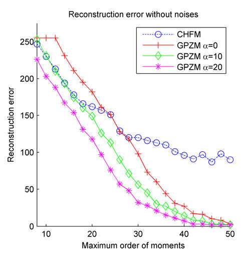
Plot of reconstruction error for the Chinese character without noise

We then test the robustness of GPZMs in the presence of noise. To do this, we add respectively 5% and 10% of salt-and-pepper noise to the original image “E”, as shown in Figs. 5 and 6. The reconstruction errors for these two cases are shown in Figs. 7 and 8, respectively. The results show that the GPZMs with larger value of α produce less error when the maximum order of moments M is relative lower. Conversely, when the maximum order of moments used in the reconstruction is higher, the reconstruction error re-increases for larger value of α. This may be because the term (1 − r)^α/2 appeared in the weighted radial polynomials is more sensitive to noise for large value of α. Another phenomenon that can be observed from these figures is that for a fixed value of α, the reconstruction error increases when the maximum order of moments M is higher. This is consistent with the conclusion made in the papers by Pawlak et al.^{15, 16} The reason is that higher order moments contribute to noise reconstruction rather than to the image.

Fig. 5.

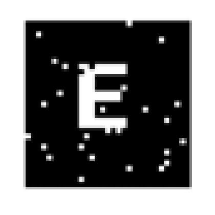
“E” added with 5% salt and pepper noises

Fig. 6.

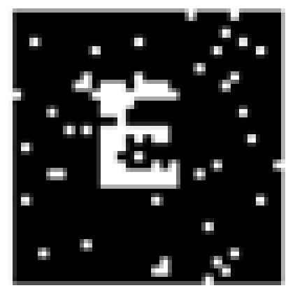
“E” added with 10% salt and pepper noises

Fig. 7.

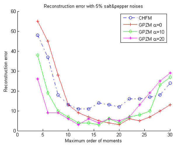
Reconstruction error for “E” with 5% salt and pepper noises

Fig. 8.

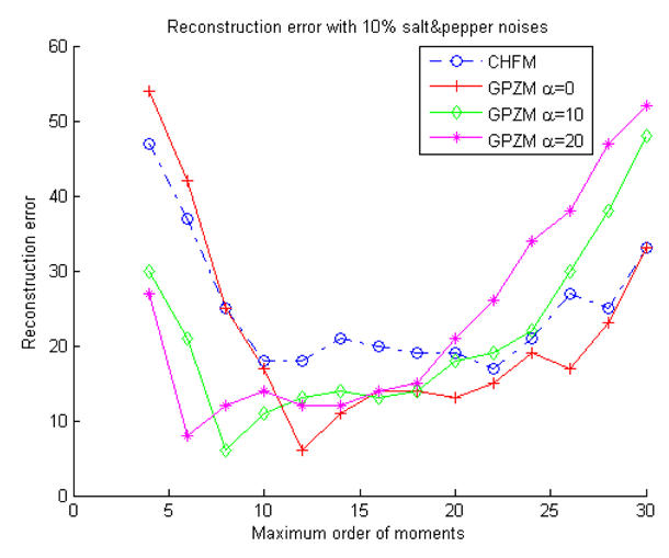
Reconstruction error for “E” with 10% salt and pepper noises

B. Invariant pattern recognition

This subsection provides the experimental study on the recognition accuracy of GPZMs in both noise-free and noisy conditions. From the definition of the GPZMs, it is obvious that the magnitude of GPZMs remains invariant under image rotation, thus they are useful features for rotation-invariant pattern recognition. Since the scale and translation invariance of image can be achieved by normalization method, we do not consider them in this paper. Note that it is also possible to construct the rotation moment invariants that are derived from a product of appropriate powers of GPZMs¹⁷. However, the moment invariants constructed in such a way will have a large dynamic range, this may cause problem in pattern classification. In our recognition task, we have decided to use the following feature vector taken into account the symmetry property of radial polynomials ${\overline{R}}_{pq}^{\alpha }(r)$

$$\mathbf{V}=[\mid {\overline{Z}}_{20}^{\alpha }\mid ,\mid {\overline{Z}}_{21}^{\alpha }\mid ,\mid {\overline{Z}}_{22}^{\alpha }\mid ,\mid {\overline{Z}}_{30}^{\alpha }\mid ,\mid {\overline{Z}}_{31}^{\alpha }\mid ,\mid {\overline{Z}}_{32}^{\alpha }\mid ,\mid {\overline{Z}}_{33}^{\alpha }\mid ]$$ (32)

where ${\overline{Z}}_{pq}^{\alpha }$ are the weighted GPZMs defined by Eq. (24). The Euclidean distance is utilized as the classification measure

$$d({\mathbf{V}}_{\mathbf{s}},{{\mathbf{V}}_{\mathbf{t}}}^{(\mathbf{k})})=\sum _{j=1}^T{(v_{sj}-{v_{tj}}^{(k)})}^2$$ (33)

where V_s is the T-dimensional feature vector of unknown sample, and V_t^(k) is the training vector of class k. The minimum distance classifier is used to classify the images. We define the recognition accuracy η as ¹⁸

$$\eta =\frac{\text{Number\hspace{0.17em}of\hspace{0.17em}correctly\hspace{0.17em}classified\hspace{0.17em}images}}{\text{The\hspace{0.17em}total\hspace{0.17em}number\hspace{0.17em}of\hspace{0.17em}images\hspace{0.17em}used\hspace{0.17em}in}\hspace{0.17em}\text{the\hspace{0.17em}test}}\times 100\%$$ (34)

Two experiments are carried out. In the first experiment, a set of similar binary Chinese characters shown in Fig. 9 is used as the training set. Six testing sets are used, each with different densities of salt-and-pepper noises added to the rotational version of each character. Each testing set consists of 120 images, which are generated by rotating the training images every 15 degrees in the range [0, 360) and then by adding different densities of noises. Fig. 10 shows some of the testing images. The feature vector based on the weighted GPZMs with different values of parameter α is used to classify these images and the corresponding recognition accuracy is compared. The results of the classification are depicted in Table 4. One can see from this table that 100% recognition results are obtained, with α being 18 or 20, for noise-free images. Note that the recognition accuracy decreases when the noise is high. Table 4 shows that the better recognition accuracy can be achieved for α between 20 to 30, and the corresponding results are much better than those with CHFMs.

Fig. 9.

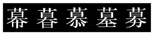
Binary images as training set for rotation invariant character recognition in the first experiment

Fig. 10.

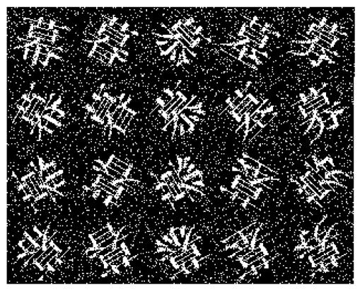
Part of the images of the testing set with 15% salt and pepper noises in the first experiment

Table 4.

Classification results of the first experiment

Parameter α for GPZMs	Recognition accuracy (%) under different salt and pepper noises
	noise free	5%	9%	10%	15%	18%
0	93.3333	60.8333	48.3333	41.6667	41.6667	36.6667
2	93.3333	86.6667	55.83333	50.8333	31.6667	30.8333
4	93.3333	59.1667	25.83333	23.3333	20.0000	20.0000
6	96.6667	55.0000	29.1667	25.0000	20.0000	20.0000
8	96.6667	59.1667	25.0000	24.1667	20.0000	20.0000
10	96.6667	94.1667	81.6667	66.6667	33.3333	30.0000
12	96.6667	85.8333	57.5000	48.3333	38.3333	36.6667
14	93.3333	75.8333	32.5000	30.8333	22.5000	20.0000
16	96.6667	81.6667	45.0000	37.5000	25.0000	20.8333
18	100	85.0000	69.1667	59.1667	42.5000	27.5000
20	100	86.6667	79.1667	67.5000	55.0000	45.0000
22	96.6667	88.3333	80.8333	71.6667	60.8000	50.8333
24	96.6667	91.6667	87.5000	75.0000	67.5000	58.3333
26	96.6667	91.6667	90.8333	79.1667	71.6667	60.8333
28	96.6667	90.8333	91.6667	78.3333	70.0000	62.5000
30	93.3333	85.0000	84.1667	74.1667	70.0000	59.1667
CHFMs	100	60	40	60	40	40

In the second experiment, we use a set of grayscale images composed of some Arab numbers and uppercase English characters {0, 1, 2, 5, I, O, Q, U, V} as training set (see Fig. 11). The reason for choosing such a character set is that the elements in subset {0, O, Q}, {2, 5}, {1, I} and {U, V} can be easily misclassified due to the similarity. Five testing sets are used, which are generated by adding different densities of Gaussian white noises to the rotational version of images in the training set. Each testing set is composed of 216 images. Fig. 12 shows some of the testing images, and the classification results are depicted in Table 5. Table 5 shows that the better results are obtained with α varying from 24 to 30.

Fig. 11.

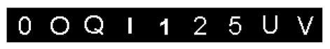
Grayscale Images of the training set used in the second experiment

Fig. 12.

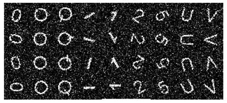
Part of the images of the testing set with σ² = 0.10 Gaussian white noises in the second experiment

Table 5.

Classification results of the second experiment

Parameter α for GPZMs	Recognition accuracy (%) under different σ2 Gaussian white noises
	noise free	0.01	0.03	0.05	0.10
0	100	83.7963	62.0370	44.4444	22.2222
2	100	99.0741	90.2778	77.7778	46.7593
4	100	96.7593	52.3148	31.4815	21.7593
6	100	94.9074	30.0926	6.94444	0
8	100	93.0556	32.8704	17.5926	12.5
10	100	99.5370	57.4074	33.7963	13.8889
12	100	100	74.5370	43.5185	23.1481
14	100	100	87.0370	66.2037	43.0556
16	100	100	95.8333	62.5000	46.2963
18	100	100	96.7593	84.2593	67.5926
20	100	100	98.1481	93.5185	65.2778
22	100	100	99.5370	96.7593	68.0556
24	100	100	100	96.2963	70.3704
26	100	100	100	97.2222	73.1481
28	100	100	100	98.6111	77.7778
30	100	100	100	98.6111	81.4815
CHFMs	100	100	77.7778	55.5556	22.2222

4. Conclusion

We have presented a new type of orthogonal moments based on the generalized pseudo-Zernike polynomials for image description. We showed that the proposed moments are an extension of the conventional pseudo-Zernike moments, and are more suitable for image analysis. Experimental results demonstrated that the generalized pseudo-Zernike moments perform better than the traditional pseudo-Zernike moments and Chebyshev-Fourier moments in terms of rotation invariant pattern recognition accuracy and image reconstruction error in both noise-free and noisy conditions. Therefore, GPZMs could be useful as new image descriptors.

References

- 1.Prokop RJ, Reeves AP. A survey of moment-based techniques for unoccluded object representation and recognition. Comput Vision Graph Image Process. 1992;54:438–460. [Google Scholar]
- 2.Hu MK. Visual pattern recognition by moment invariants. IRE Trans Inf Theory. 1962;IT-8:179–187. [Google Scholar]
- 3.Dudani S, Breeding K, McGhee R. Aircraft identification by moment invariants. IEEE Trans Comput. 1977;26:39–45. [Google Scholar]
- 4.Belkasim SO, Shridhar M, Ahmadi M. Pattern recognition with moment invariants: A comparative study and new results. Pattern Recognit. 1991;24:1117–1138. [Google Scholar]
- 5.Markandey V, Figueiredo RJP. Robot sensing techniques based on high dimensional moment invariants and tensor. IEEE Trans Robot Automat. 1992;8:186–195. [Google Scholar]
- 6.Teague MR. Image analysis via the general theory of moments. J Opt Soc Am. 1980;70:920–930. [Google Scholar]
- 7.Teh CH, Chin RT. On image analysis by the methods of moments. IEEE Trans Pattern Anal Mach Intell. 1988;10:496–513. [Google Scholar]
- 8.Ping ZL, Wu RG, Sheng YL. Image description with Chebyshev-Fourier moments. J Opt Soc Am A. 2002;19:1748–1754. doi: 10.1364/josaa.19.001748. [DOI] [PubMed] [Google Scholar]
- 9.Sheng YL, Shen LX. Orthogonal Fourier-Mellin moments for invariant pattern recognition. J Opt Soc Am A. 1994;11:1748–1757. [Google Scholar]
- 10.Mukundan R, Ramakrishnan KR. Moment Functions in Image Analysis-Theory and Application. World Scientific; Singapore: 1998. [Google Scholar]
- 11.Wünsche A. Generalized Zernike or disc polynomials. J Comp App Math. 2005;174:135–163. [Google Scholar]
- 12.Dunkl CF, Xu Y. Orthogonal polynomials of several variables. Cambridge University Press; Cambridge: 2001. [Google Scholar]
- 13.Chong CW, Raveendran P, Mukundan R. The scale invariants of pseudo-Zernike moments. Pattern Anal Appl. 2003;6:176–184. [Google Scholar]
- 14.Chong CW, Raveendran P, Mukundan R. A comparative analysis of algorithms for fast computation of Zernike moments. Pattern Recognit. 2003;36:731–742. [Google Scholar]
- 15.Liao SX, Pawlak M. On image analysis by Moments. IEEE Trans Pattern Anal Mach Intell. 1996;18:254–266. [Google Scholar]
- 16.Liao SX, Pawlak M. On the accuracy of Zernike Moments for Image Analysis. IEEE Trans Pattern Anal Mach Intell. 1998;20:1358–1364. [Google Scholar]
- 17.Flusser J. On the independence of rotation moment invariants. Pattern Recognit. 2000;33:1405–1410. [Google Scholar]
- 18.Yap PT, Raveendran P, Ong SH. Image analysis by Krawtchouk moments. IEEE Trans Image Process. 2003;12:1367–1377. doi: 10.1109/TIP.2003.818019. [DOI] [PubMed] [Google Scholar]