How long to scan? The relationship between fMRI temporal signal to noise and necessary scan duration

Abstract

Recent advances in MRI receiver and coil technologies have significantly improved image signal-to-noise ratios (SNR) and thus temporal SNR (TSNR). These gains in SNR and TSNR have allowed the detection of fMRI signal changes at higher spatial resolution and therefore have increased the potential to localize small brain structures such as cortical layers and columns. The majority of current fMRI processing strategies employ multi-subject averaging and therefore require spatial smoothing and normalization, effectively negating these gains in spatial resolution higher than about 10mm³. Reliable detection of activation in single subjects at high resolution is becoming a more common desire among fMRI researchers who are interested in comparing individuals rather than populations. Since TSNR decreases with voxel volume, detection of activation at higher resolutions requires longer scan durations. The relationship between TSNR, voxel volume and detectability is highly non-linear. In this study, the relationship between TSNR and the necessary fMRI scan duration required to obtain significant results at varying P values is determined both experimentally and theoretically. The results demonstrate that, with a TSNR of 50, detection of activation of above 2% requires at most 350 scan volumes (when steps are taken to remove the influence of physiological noise from the data). Importantly, these results also demonstrate that, for activation magnitude on the order of 1%, the scan duration required is more sensitive to the TSNR level than at 2%. This study showed that with voxel volumes of ~10mm³ at 3T, and a corresponding TSNR of ~50, the required number of time points that guarantees detection of signal changes of 1% is about 860, but if TSNR increases by only 20%, the time for detection decreases by more than 30%. More than just being an exercise in numbers, these results imply that imaging of columnar resolution (effect size = 1% and assuming a TR of 1sec) at 3T will require either 10 minutes for a TSNR of 60 or 40 minutes for a TSNR of 30. The implication is that at these resolutions, TSNR is likely to be critical for determining success or failure of an experiment.

Introduction

Functional magnetic resonance imaging (fMRI) has advanced the field of brain research by enabling imaging of brain function with relatively high spatial resolution and speed. Noise in the data necessitates signal averaging to extract functional information, which is manifest as signal changes on the order of a few percent. A natural development in fMRI is towards high spatial resolution, which presents unique opportunities as well as challenges.

Regarding opportunities, studies have demonstrated that distinctive functional information is present at a resolution on the order of 1.5mm³ (Cheng et al., 2001; Hyde et al., 2001; Kim et al., 2000; Logothetis et al., 2002; Menon et al., 1997). This functional information has been shown to correspond to functional units on the scale of cortical columns and appears to give, within the spatial pattern of activation, a unique insight into how the brain processes information. Accurate detection of activation in a single subject at high-resolution has significant promise and could play a critical role in a clinical setting for pre-surgical mapping and diagnosis where individual differences in brain function are crucial. Advances in the study of smaller structures in the brain such as columns and layers will help our understanding of the organization of neuronal populations and their interactions with each other. Recent techniques in fMRI that examine patterns of activation (Beauchamp et al., 2004; Haxby et al., 2001; Haynes and Rees, 2005; Kamitani and Tong, 2005; Kriegeskorte et al., 2006) should also benefit from reliable high-resolution single subject activation maps. Higher resolution is also desirable for practical reasons such as the reduction in signal dropout due to less macroscopic, susceptibility related intra-voxel dephasing and for the purposes of brain segmentation (Bellgowan et al., 2006; Bodurka et al., 2006).

Regarding challenges of high-resolution imaging, the process of spatial normalization and intrasubject spatial averaging reduces spatial resolution to the order of 10mm³, therefore imaging at high spatial resolution is currently only performed in a single subject basis. Second, but most important since MRI signal to noise (SNR) is directly proportional to voxel volume (Edelstein et al., 1986), fMRI detection power decreases as voxel volume decreases. Therefore, improvements in spatial resolution require either higher SNR or longer scan time. In this study, a framework for working within practical limits established by SNR, resolution and scanning time, is determined.

Noise present in fMRI time course data has physiological, thermal and scanner-related or system contributions (Kruger and Glover, 2001) and is a major obstacle to detecting activation in a single time series. In the context of MRI, Signal-to-Noise Ratio (SNR) reflects static or single image MRI signal ratio over the noise present in the absence of signal. However, it does not provide insight into the temporal noise characteristics of fMRI time courses. A useful measure of image time course stability is the Temporal Signal-to-Noise Ratio (TSNR) calculated by dividing the mean of a time series by its standard deviation. The non-linear relationship between TSNR and SNR in gradient recalled EPI BOLD data has been experimentally shown and a physiological noise model in oxygenation-sensitive fMRI has been introduced (Kruger and Glover, 2001; Kruger et al., 2001). The relative fraction of physiologic noise increases linearly as a function of SNR, hence the Krueger and Glover noise model predicts that as image SNR increases, TSNR in oxygenation-sensitive MRI BOLD signal saturates. Recently, Bodurka and colleagues, taking advantage of a substantial 3-fold SNR increase offered by a multi-channel MRI receiver and a sensitive 16-element brain surface coils array, demonstrated this asymptotic behavior at 3 Tesla (Bodurka et al., 2005). Both these results and those of Krueger and Glover derive TSNR limits of 78–90, 110–160 and 47–55 for physiological noise contributions at 3T for gray matter (GM), white matter (WM) and cerebral-spinal fluid (CSF) respectively (Bodurka et al., 2004; Bodurka et al., 2005; Kruger and Glover, 2001). Figure 1 shows a schematic of the relationship between SNR and TSNR in gray matter using this limit. Estimates of SNR derived from values reported by Triantafyllou and colleagues for 1.5T, 3T and 7T scanners (equipped with standard head coils) at resolutions of 1mm³, 8mm³ and 27mm³ are also shown.

Figure 1.

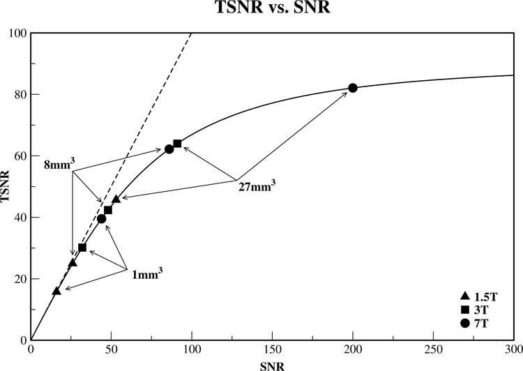
A schematic of the relationship between TSNR and SNR in gray matter is shown. The dashed line represents this relationship in the absence of physiological noise. In vivo, gains in TSNR are limited by physiological noise as SNR is increased and this relationship is displayed with the solid line. For gray matter, the TSNR limit is approximately 87 (Bodurka et al., 2005). Using values derived from those reported by Triantafyllou and colleagues (Triantafyllou et al., 2005), estimates of SNR for 1.5T, 3T and 7T scanners equipped with standard head coils are shown for voxel sizes of 1×1×1mm³ = 1mm³, 2×2×2mm³ = 8mm³ and 3×3×3mm³ = 27mm³.

The presence of noise in fMRI data necessities the use of statistical measures to determine levels of brain activation. To achieve the required statistical power, tasks are repeated, efficient experimental designs are utilized and large groups of subjects are typically averaged together in normalized space. The issue of optimizing these parameter has been approached in several studies: the number of subjects required (Desmond and Glover, 2002; Friston et al., 1999; Murphy and Garavan, 2004), the effects of experimental design on detection and response estimation (Birn et al., 2002; Liu et al., 2001) and the number of blocks/events required (Huettel and McCarthy, 2001; Murphy and Garavan, 2005; Saad et al., 2003). Detection of activation in a single time series poses unique problems with the need for statistical power to be increased by other means. For example, it has been shown that activation detection is optimized using a 50% duty cycle and a block design works best (Birn et al., 2002; Liu et al., 2001). Saad and colleagues have shown that when multiple scans of block design are averaged together, there is a monotonic increase in statistical significance as the number of scans increases (Saad et al., 2003). This, in effect, is similar to increasing TSNR in a time series since the effects of noise are reduced by the temporal averaging method used. This is particularly relevant at higher spatial resolution, as discussed above, where physiological noise contribution decreases and the relationship between TSNR and SNR becomes more linear (Bodurka et al., 2005; Kruger and Glover, 2001; Triantafyllou et al., 2005). This suggests that increasing SNR, and thus TSNR, by utilizing hardware improvements will improve the ability to detect activation in a single time series at higher spatial resolutions. However, for a given scanner hardware and MRI signal reception setup, the only remaining option to improve statistical power in a high-resolution activated fMRI voxel is to increase the length of the time series.

To investigate small-scale structures of ~1mm size that exist in the brain, detection of activation in high-resolution single voxel time series is required. This study, through theory, simulated and experimental data, characterizes the relationship between TSNR and the necessary scan duration to reliably detect activation in a single voxel with a given fractional signal change. With a measure of TSNR and the expected fractional signal change with activation, an experimenter can use derived relationship from this paper to determine the scan duration required to yield sufficient power to detect that activity in high-resolution fMRI images.

Theory

What follows is the derivation of an equation that relates TSNR to scan duration, measured in number of time points N, taking into account the size of the effect, eff, and the significance to which we would like to detect it, P. The temporal signal-to-noise ratio, TSNR, of a time series x_i is defined by:

$$\mathit{\text{TSNR}}=\frac{\mu }{\sigma }=\frac{\mu }{\sqrt{\raisebox{1ex}{$1$}\!\left/ \!\raisebox{-1ex}{$N$}\right.{\displaystyle \sum _{i=1}^N{(x_i-\mu )}^2}}}$$ (1)

where N is the number of time points, µ is the mean of the time series and σ is its standard deviation. The correlation coefficient is defined as:

$$\mathit{\text{cc}}=\frac{{\displaystyle \sum _{\mathrm{i}=1}^{\mathrm{N}}{x}_i{y}_i-N{\mu }_x{\mu }_y}}{\sqrt{\left[{\displaystyle \sum _{\mathrm{i}=1}^{\mathrm{N}}{(x_{\mathrm{i}}-{\mu }_x)}^2}\right]\hspace{0.17em}\left[{\displaystyle \sum _{\mathrm{i}=1}^{\mathrm{N}}{(y_{\mathrm{i}}-{\mu }_y)}^2}\right]}}$$ (2)

where x_i represents the measured time series in a voxel, y_i is the reference or ideal time series, i = 1, 2, … N where N is the number of time points, µ_x and µ_y are the mean values of x_i and y_i respectively. If we assume that y_i=1 for half of i = 1, 2, … N and y_i=0 for the other half, that the mean in the ON period is equal to (1+eff) times the mean in the OFF period and that the standard deviation in the ON and OFF periods are equal then Eq. 2 simplifies to:

$$\mathit{\text{cc}}=\mathit{\text{TSNR}}\left(\raisebox{1ex}{$\mathit{\text{eff}}$}\!\left/ \!\raisebox{-1ex}{$2$}\right.\right)$$ (3)

It is possible to convert cc values to P values, thus introducing a dependence on the number of time points N, by using Eq. 4:

$$P=1-\frac{2}{\sqrt{\pi }}{\displaystyle {\int }_0^{\mathit{\text{cc}}\sqrt{N/2}}{e}^{-t^2}}\mathit{\text{dt}}=\mathit{\text{erfc}}(\mathit{\text{CC}}\sqrt{N/2})$$ (4)

where erfc is the complementary error function.

Substituting 2 into 3 and solving gives

$$\mathit{\text{TSNR}}=\sqrt{\raisebox{1ex}{$8$}\!\left/ \!\raisebox{-1ex}{$N$}\right.}\left(\raisebox{1ex}{$1$}\!\left/ \!\raisebox{-1ex}{$\mathit{\text{eff}}$}\right.\right){\mathit{\text{erfc}}}^{-1}\left(P\right)$$ (5)

where erfc⁻¹ is the inverse complementary error function.

This can be rewritten to give the number of time points required when we know the TSNR and effect size:

$$N=8{\left(\frac{{\mathit{\text{erfc}}}^{-1}\left(P\right)}{\left(\mathit{\text{TSNR}}\right)\left(\mathit{\text{eff}}\right)}\right)}^2$$ (6)

This equation can be generalized to situations in which the ON period is not exactly half the length of the time series. Let R be the ratio of the time points in the ON period to the total number of time points and 0<R<1. Then Eq. 6 becomes

$$N=\frac{2}{R\left(1-R\right)}{\left(\frac{{\mathit{\text{erfc}}}^{-1}\left(P\right)}{\left(\mathit{\text{TSNR}}\right)\left(\mathit{\text{eff}}\right)}\right)}^2$$ (7)

Methods

To investigate the relationship between TSNR and scan duration and to verify the validity of the theoretically derived equations, four datasets were employed. The first dataset comprised of simulated time series, the second of resting state scans, the third of similar scans with a visual task presentation, and the final dataset consisted of two 30 minute long resting state scans. Details of these datasets and the subsequent analyses are given below.

Simulations

Dataset 1

Simulated time series lasting 1800 time points (1800 time points corresponds to 60 minutes if TR=2sec), each with a specific TSNR, were generated by selecting time points from a Gaussian distribution. This was performed 100 times for each level of TSNR in 1, 2, …, 150 (150 being a rough upper bound of TSNR (Bodurka et al., 2005) when post processing techniques are not used) yielding a total of 15,000 time series. Each of these time series was used to create another 60 time series of increasing length, by taking the first 30, 60, 90, …, 1800 time points (corresponding to 1, 2, …, 60 minutes for TR=2sec). This resulted in a total of 900,000 time series.

Imaging Hardware and Protocols

Six subjects (S1, S2, …, S6) were scanned on a 3T General Electric Signa Excite MRI scanner (3T/90cm, whole body gradient inset 40mT/m, slew rate 150 T/m/s, whole body RF coil, 16 fast digital receivers) equipped with an 8-element receive only GE head surface coils array. Single-shot full k-space gradient echo EPI images with matrix size of 128×128 were acquired.

Dataset 2

Five resting scans were acquired for each of the first 5 participants, S1, S2, …, S5. Fourteen contiguous slices were acquired in the axial plane with imaging parameters: FOV/slice 22cm/4mm, TR=2sec, TE=45ms, number of volumes=190. For S1, S2 and S3, the flip angle was kept constant at 90°. For S4 and S5, the flip angle was varied for each scan: 90°, 70°, 45°, 20° and 10° producing a greater variation in image SNR and therefore TSNR across scans.

Dataset 3

Five visual task scans, interspersed between the resting scans, were also acquired on S3, S4 and S5 with similar parameters. As in the resting state scans, the flip angle was held constant for S3 and varied for S4 and S5. The task consisted of fixation in the center of a contrast-reversing black-and-white checkerboard flashing at 8Hz. This visual stimulus was presented in a block design with 30secs OFF/30secs ON for the duration of the scan.

Dataset 4

With subject S6, two 30 minute resting scans were acquired, each at a different resolution. On the lower resolution scan, similar parameters to the resting state scans above were used: FOV/slice 22cm/4mm, TR=2sec, TE=45ms, flip=90°, number of volumes=1800. The resolution was increased for the second scan by decreasing the slice thickness to 1mm. All other parameters were identical to those used in the first scan.

Data Analysis

The AFNI software package (http://afni.nimh.nih.gov/afni) was utilised (Cox, 1996). The resting state and visual task fMRI data were 3D volume registered. The visual data were also time shifted to align separate slices to the same temporal origin. For S1, S2 and S3, the five resting state scans were concatenated into one (first removing the means and the linear trends of each scan, then reintroducing the global mean after concatenation). Thirty resting state datasets of increasing length were derived for each subject from this concatenated dataset by taking the first 30 time points (corresponding to 1 minute), the first 60 time points (corresponding to 2 minutes), etc., up to all 1800 time points (corresponding to 30 minutes). This approach retains any autocorrelations that were present in the original data. The linear and quadratic trends were also removed from both of S6’s resting state scans (Dataset 4).

Artificial block activations with effect sizes of 0.1%, 0.2% …, 1.0%, 2.0%, …, 5.0% were injected into the simulated time series (Dataset 1) and all voxels in the resting state scans (Dataset 2 and 4). These block activations consisted repetitions of 15 time points OFF and 15 time points ON (corresponding to 30secs OFF/30secs ON if TR=2sec) and were convolved with a hemodynamic Gamma-variate impulse response function (assuming TR=2sec) (Cohen, 1997). Correlation analyses were performed on all resulting time series, both simulated (Dataset 1) and experimental (Dataset 2 and 4). The correlation coefficient with the ideal block regressor was calculated for each time series and converted to a P value (Eq. 4).

The TSNR was computed for each simulated time series and in every voxel of each resting scan by calculating the mean and standard deviation of the time points (before the insertion of the effect and after dropping the first 5 images to allow steady state to be reached) and taking their ratio.

The visual task data (Dataset 3) were analyzed using the same correlation approach. A mask of the visual areas was calculated by thresholding the correlation maps at 0.365 corresponding to P = 5×10⁻⁷. The effect size of the visual activation was calculated by using the same block regressor in a multiple regression technique along with nuisance regressors to remove the effects of linear drifts and movement. Two values of TSNR were calculated for these datasets. The first simply takes the TSNR values from the preceding rest scan to give TSNR_rest. For the second, the activation was removed from each voxel by removing the mean and the linear trend of the OFF periods from the data, scaling the block regressor to the calculated effect size, subtracting this scaled regressor from the data and then reintroducing the mean of the OFF periods into the time series. The task TSNR_task value was calculated using this modified time series.

Scan Duration vs. TSNR

The relationship between Scan Duration and TSNR was calculated using the theory. By inserting P = 0.05, 0.005, …, 5×10⁻¹⁰ and eff = 0.001, 0.002, …, 0.01, 0.02, …, 0.05 for each N = 30, 60, …, 1800 into Eq. 5, the corresponding TSNR_T at which activation can be detected was determined (the T subscript denotes that this value was derived from the theory). A plot of TSNR_T vs. N could then be used to determine how many time points are required to detect activation with an effect size eff to a specific P value when the TSNR is known.

Similar relationships were determined using the simulated time series (Dataset 1). For each effect size (0.1%, 0.2%, …, 1.0%, 2.0%, … 5.0%) and number of time points (30, 60, …, 1800), there are 100 runs, each with 150 time series corresponding to TSNRs of 1,2, …, 150. One difference between the theory and simulated data is that the theory assumes a perfectly sampled Gaussian distribution but since the simulated time series are finite, perfect sampling of this distribution is not possible. Therefore, if a time series of length N has a TSNR equal to a specific TSNR_T, the P value to which activation is detected may not correspond to that determined by the theory. By chance, it would be higher 50% of the time and lower the other 50%. For a given effect size, number of time points and P value, the first TSNR level in 1,2, …, 150 that displayed 50 of the 100 runs passing the threshold was called TSNR_C. Thus, TSNR_C should correspond to the theory, that is, TSNR_C should equal TSNR_T. However, a more useful measure would be one that guarantees activation detection, TSNR_G. This was determined by finding the first TSNR in 1,2, …, 150 that all 100 runs passed the significance level. By plotting TSNR_G against N, for each P value and effect size, one can determine how many time points are required to guarantee activation detection according to the simulations.

For all resting state data (Dataset 2 and 4), a similar TSNR_G measure was calculated. The data were thresholded at each P value for each effect size and scan duration. The resting state TSNR maps were sequentially thresholded at TSNR levels of 1, 2, …, 150. The TSNR value at which this thresholded map became entirely a subset of the thresholded activation map was called TSNR_G. Thus, every voxel with a value of TSNR above TSNR_G detected activation to the corresponding P value for that specific effect size and scan duration.

Results

The theoretical equation (Eq. 6) can be used to determine how many time points are required to detect activation. Plots of this equation are shown in Figure 2 for various effect sizes when activation is to be detected to a liberal (P = 0.05, top graph) and a strict (P = 5×10⁻¹⁰, bottom graph) threshold. For example, if a time series has a TSNR = 75, to detect activation with an effect size of 0.5% to a threshold of P = 0.05, ~110 time points are required according to the theory. However, if a stricter threshold of P = 5×10⁻¹⁰ is necessary, the number of time points must to be increased to ~1100.

Figure 2.

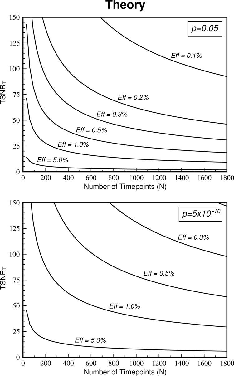
The theoretical relationship between TSNR_T and number of time points, N, is shown. The top graph depicts this relationship for various effect sizes when a liberal threshold of P = 0.05 is required. The bottom graph shows the same information for a conservative threshold of P = 5×10⁻¹⁰.

The TSNR_C results derived from the simulations should give values that correspond very closely to the theory. Figure 3 shows these values for various effect sizes at both P = 0.05 and P = 5×10⁻¹⁰ thresholds. The corresponding theoretically derived curves are plotted with dotted lines. For the P = 0.05 case, the TSNR_C values correspond almost perfectly to the theory. At P = 5×10⁻¹⁰, the TSNR_C values are slightly increased beyond the theory values with this increase becoming greater for smaller effect sizes. For example, at TSNR = 125, the theory suggests that ~1100 time points are required to detect a 0.3% effect size compared to the simulations 1200 time points. This is an increase of only 9% and suggests that the TSNR_C values might have a small bias to over-estimating the required number of time points at strict P values with small effect sizes.

Figure 3.

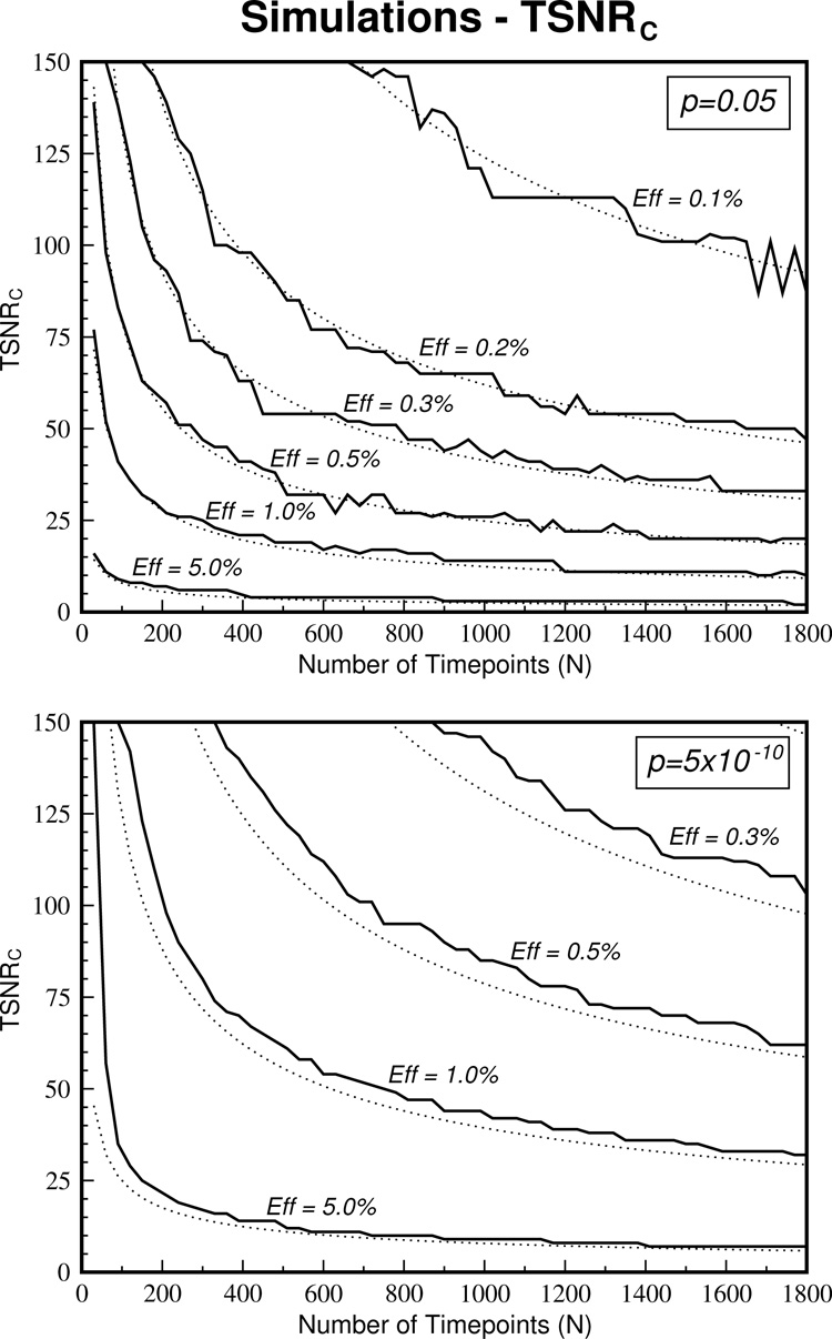
A comparison of the simulated TSNR_C values with the corresponding theoretical curves is shown. The TSNR_C curves (solid lines) match the theoretical curves (dotted lines) almost perfectly for a liberal threshold of P = 0.05 (top graph) and give only slightly increased values for the strict threshold of P = 5×10⁻¹⁰.

The simulations can be used to determine the TSNR that guarantees activation detection when the number of time points is known. These TSNR_G curves are plotted in Figure 4 and are compared to the corresponding theoretical curves (dotted lines). The number of time points required to guarantee activation detection is much greater than those derived from the theory. For example, at a TSNR = 50, the theory suggests that an effect size of 0.3% can be detect in ~700 time points (at least to the liberal threshold of P = 0.05). However, according to the TSNR_G measure, one would not be guaranteed to detect this activation no matter how long one scanned and even detection of an effect size of 0.5% is not guaranteed with this number of time points.

Figure 4.

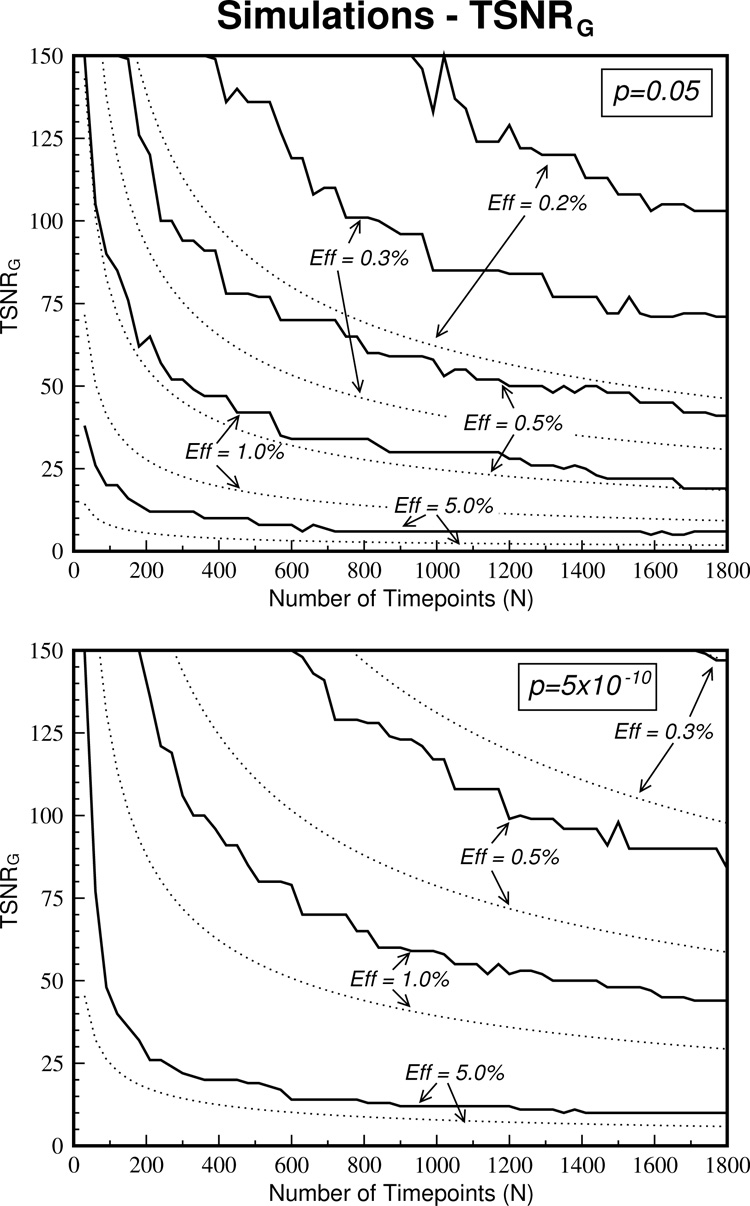
The TSNR values that guarantee activation (TSNR_G) according to the simulations are shown with the solid line. The corresponding theoretical curves are shown with dotted lines. Simulated TSNR_G values are greatly elevated above the theoretically derived values.

Comparisons with real noise data collected during rest show that the TSNR_G curves derived from the data are higher than those derived from the simulations. This is illustrated in Figure 5 where the curves from the concatenated datasets (Dataset 2) are shown in the solid lines and their corresponding simulated curves are dotted. This discrepancy between the curves could have two causes. First, whilst all care has been take to remove means and linear trends from datasets before concatenation, this operation can introduce discontinuities in the time series that might affect the calculation of TSNR and the correlation analysis. Second, deviations from Gaussian noise due to the inclusion of physiological noise, which introduces autocorrelation into the time series, could skew the results.

Figure 5.

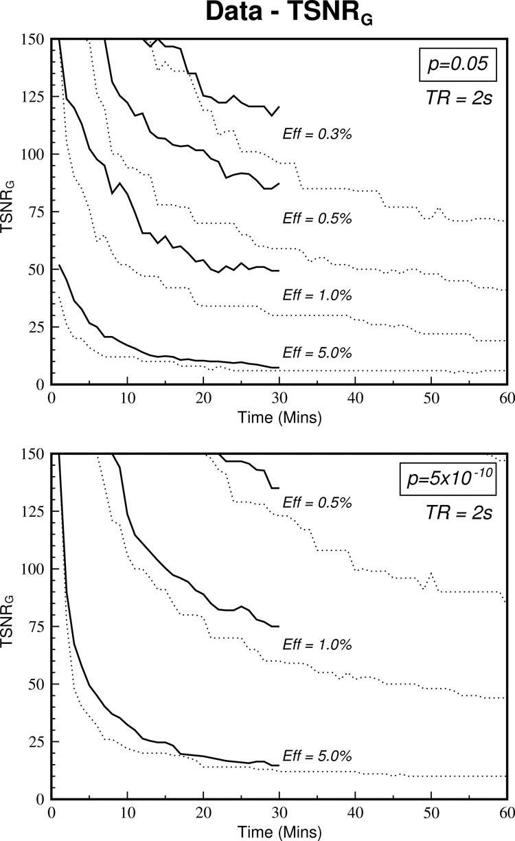
The relationship between TSNR_G and scan duration for the concatenated resting state datasets (averaged across S1, S2 and S3) is shown with the solid lines. Comparison with the simulated TSNR_G values (dotted lines) show that deviation from Gaussian noise due to inclusion of physiological noise elevates the required TSNR. This effect is greater for smaller effect sizes.

To address the first issue, comparison with a continuous 30-minute dataset is shown in Figure 6. The values for higher effect sizes (>1%) remain relatively unchanged whereas for lower effect sizes (<0.5%), the Data TSNR_G curves are brought closer to the simulated curves. This is consistent with the fact that concatenation can introduce discontinuities with scales on the order of these small effect sizes thus skewing the results. Therefore, continuous acquisition greatly benefits smaller effect sizes but the discontinuities introduced by concatenation impinge on the larger effect sizes to a lesser degree.

Figure 6.

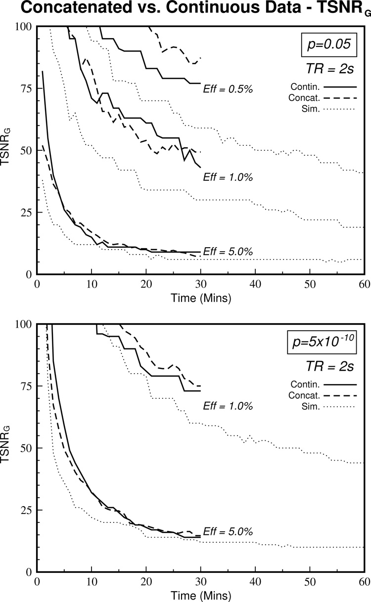
Concatenation of datasets can produce discontinuities into the time series that could adversely affect the calculation of TSNR_G. To investigate this effect, the curves derived from the concatenated datasets (see Figure 5) are shown along with the values derived from the continuous dataset at the same resolution (first scan from Dataset 4). Using continuous datasets reduces the discrepancy with the simulated values (dotted lines) for smaller effect sizes. Larger effect sizes remain reasonably unchanged, possibly since these effect sizes are much greater than the discontinuities introduced by concatenation. (Note: the scales of the Y-axes have changed from the previous figures).

The second issue, concerning autocorrelation in the data, can be addressed by removing physiological noise. As SNR decreases, the influence of physiological noise on the data decreases (see Figure 1). By going to higher resolution, SNR is inherently decreased and noise becomes more Gaussian-like thus reducing autocorrelation. A comparison was made between two 30 minute datasets, one at a resolution of ~14mm³ voxel volume and the other at ~3.5mm³. Figure 7 shows the autocorrelation functions for the data at both these resolutions averaged across all voxels in the brain. It is clear that autocorrelation in the data is reduced by going to higher resolution.

Figure 7.

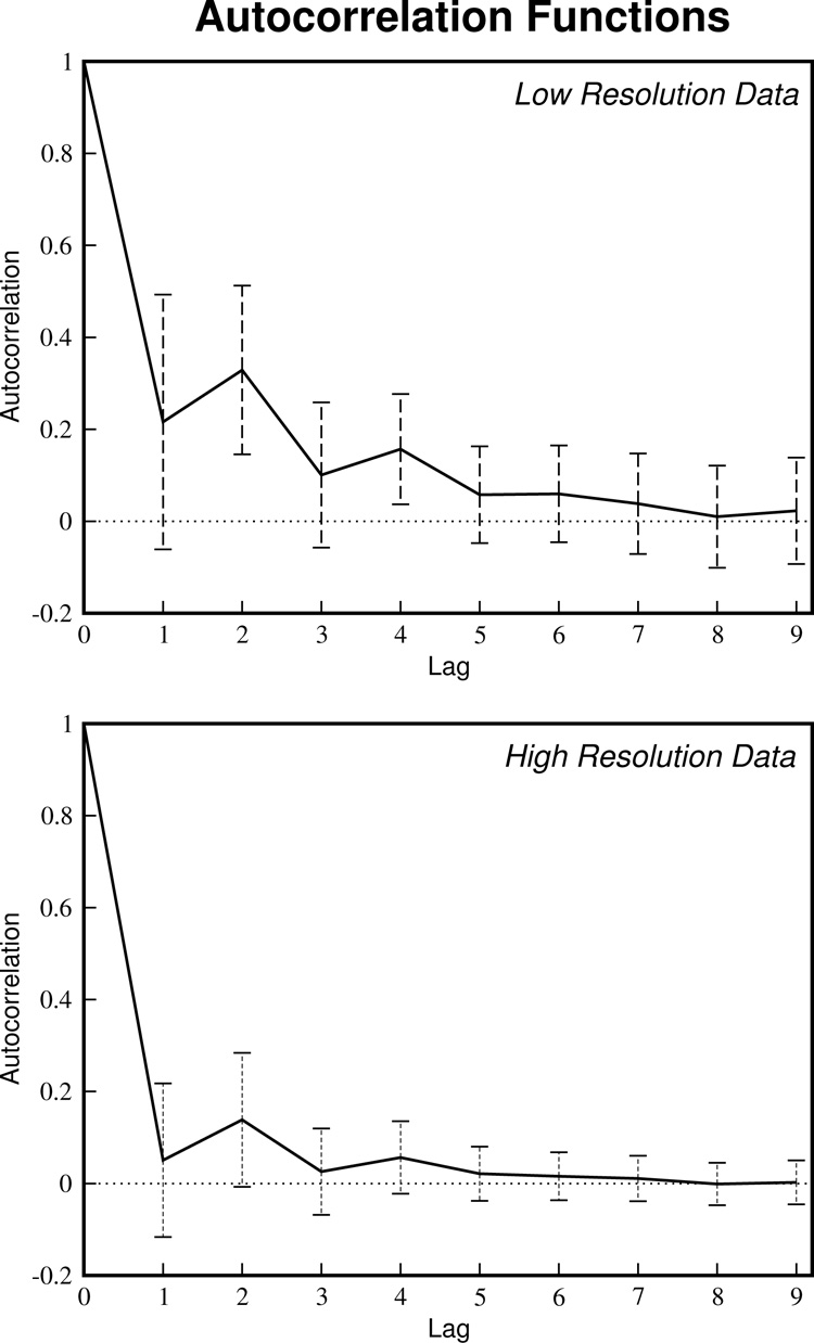
Physiologic noise introduces autocorrelation into the time series. By going to higher resolutions, the effects of physiological noise can be reduced (see Figure 1) and thus the autocorrelation will be reduced. The autocorrelation functions for both the low- and high-resolution continuous datasets (Dataset 4: 1.875mm × 1.875mm × 4mm = 14.063mm³ and 1.875mm × 1.875mm × 1mm = 3.515mm³) averaged across all voxels are shown. Increasing the resolution to these dimensions reduces the autocorrelation in the data almost to zero.

Figure 8 demonstrates how removal of autocorrelations by reducing physiological noise affects the TSNR_G curves. The high-resolution curves (solid lines) are closer to those predicted by the simulations, especially at lower effect sizes and lower scan durations.

Figure 8.

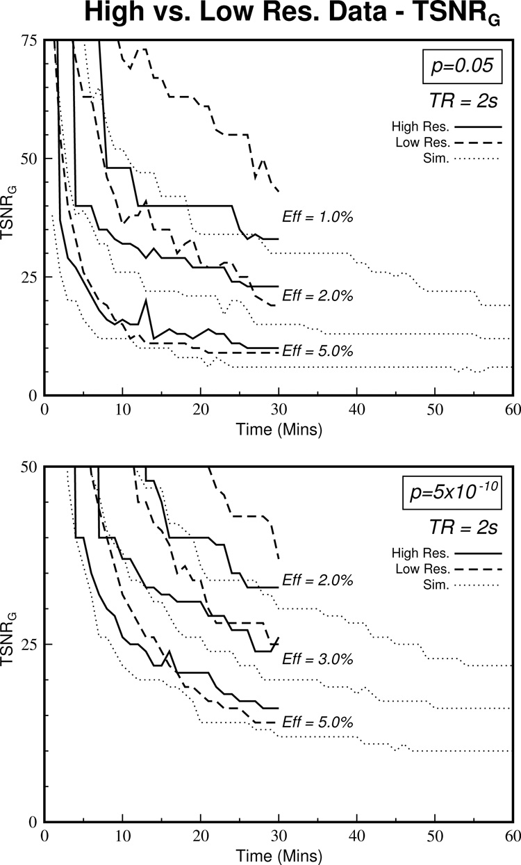
The effect of removing most of the physiologic noise by increasing the resolution can be seen. By removing physiologic noise, the datasets become more Gaussian and therefore more like the simulated curves, especially at smaller effect sizes and lower scan durations. Hence, if the influence of physiological noise can be removed by using methods such as RETROICOR, pre-whitening and higher resolution scans, the simulated data give the true relationship between required TSNR and require scan duration. (Note that the Y-axis values are different from the previous graphs since the high-resolution dataset had a maximum TSNR value of 48. This also explains the step-like structure of the upper high-resolution curves in each of the graphs due to the lack of voxels in the calculation.)

Verification of these finding with experimentally measured block activations (Dataset 3) is difficult since effect size is a continuous and constantly varying parameter across voxels. Both the simulated (Dataset 1) and experimental data (Dataset 2) utilize discrete effect size values and thus lack the continuity required to assess the validity of the results. However, it is possible to compare the acquired block activation data (Dataset 3) with the theory (and hence TSNR_C). By estimating the effect size, determining the P value of activation and knowing the scan length in the visually activated areas, one can assess whether the corresponding TSNR value agrees with Eq. 4. When inserting TSNR_rest into the equation, there is a relatively poor correspondence with theory with only 60.3% of voxels in the visual areas (collapsed across S3, S4 and S5 and all flip angles) adhering to the theory. This suggests that 39.7% of the voxels have detected activation with a TSNR value that is lower than the theoretical value. This is in line with the simulated TSNR_C measure in which 50% of voxels would detect activation with a TSNR lower than TSNR_T. However, when we use TSNR_task in Eq. 3, 99.9% of voxels have a greater TSNR that TSNR_T. Neither measures of TSNR are optimal but the results suggest that the experimentally measured block activations might correspond well to values derived by the simulations (TSNR_C).

Discussion

The results show that the theoretically derived values, TSNR_T, correspond well with the simulated values, TSNR_c, lending credence to the validity of the equations. However, these equations assume a perfect sampling of the Gaussian distribution, which is not possible in a finite time series. Hence, estimations of required scan duration derived from the theory do not guarantee that the activation in question will be detected. To attempt to overcome this problem, the TSNR_G measure was derived from the simulations, which determines the TSNR at which all 100 runs of the simulated data detect the activation. This measure yields values that are much greater than the TSNR_C measure (see Figure 4) and that are more in line with those derived from real data (see Figure 5). However, real data deviates from Gaussian noise properties due to physiological noise, which introduces autocorrelations in the data.

It has long been recognized that noise in fMRI data is non-Gaussian or non-white (Bandettini et al., 1993; Friston et al., 1995; Weisskoff et al., 1993). A major component of this deviation from Gaussianity is driven by physiological noise that increases with MRI signal as discussed above (Kruger and Glover, 2001; Kruger et al., 2001). However, in the MRI high resolution regime with voxel volumes <2mm³, signal is low and thermal noise dominates physiological noise even at high fields such as 7T (Triantafyllou et al., 2005). Thus, for higher spatial resolutions, the noise in the data appears more Gaussian. Similarly for lower resolutions, correction methods (such as RETROICOR (Glover et al., 2000) or pre-whitening (Purdon and Weisskoff, 1998)) can be used to minimize the contribution of physiological noise thus making the overall noise more Gaussian-like (Lund et al., 2006). When pushing the limits of resolution and detectability in fMRI, correction procedures like this are advantageous, however, these corrections become less relevant the higher the resolution/lower the SNR since noise is primarily dominated by thermal fluctuations at these spatial scales. By going to these higher resolutions, the influence of this noise component can be reduced, leading to curves that resemble the simulated curves more closely as demonstrated in Figure 8. Since autocorrelation is removed from the data, these results are independent of TR. Therefore, in the high-resolution regime (or when processing steps are taken to remove the influence of autocorrelation due to physiological noise from the data, rendering the noise more thermal-like (Birn et al., 2006a; Birn et al., 2006b)), the simulated measure, TSNR_G, best predicts the required number of time points to guarantee detection of activation.

If we were to use the simulated measure, TSNR_G, as the gold standard, it would be beneficial to have an equation that fits the curves well. The ratio of TSNR_G to TSNR_T changes with P value. By using non-linear fitting techniques, the following relationship was derived:

$${\mathit{\text{TSNR}}}_G=1.5\left(1+e^{{\text{log}}_{10}\raisebox{1ex}{$P$}\!\left/ \!\raisebox{-1ex}{$2$}\right.}\right){\mathit{\text{TSNR}}}_T$$ (8)

Thus, from Eq. 5, the required number of time points to guarantee detection of activation with an effect size, eff, to a statistical threshold P, for a given time series TSNR is:

$$\begin{array}{c}{N}_G=8{\left[1.5\left(1+e^{{\text{log}}_{10}\raisebox{1ex}{$P$}\!\left/ \!\raisebox{-1ex}{$2$}\right.}\right)\left(\frac{{\mathit{\text{erfc}}}^{-1}\left(P\right)}{\left(\mathit{\text{TSNR}}\right)\left(\mathit{\text{eff}}\right)}\right)\right]}^2\end{array}$$ (9)

This relationship between TSNR and N_G is plotted in Figure 9 for various effect sizes and P values. This equation and graph can be used to determine the number of time points needed to guarantee activation detection. It should be noted that detection might be possible using shorter scan durations than those derived but it is not guaranteed.

Figure 9.

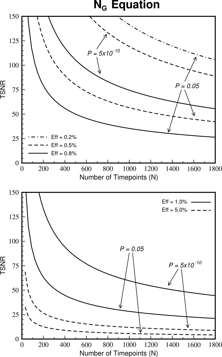
The TSNR_G values derived from the simulations can be used as a gold standard for determining the required scan duration for detecting activation. Plots of the equation that fit these data (Eq. 9) are shown for various effect sizes and P values. When acquiring in the high-resolution regime, where physiological noise is reduced and the remaining noise is close to Gaussian, these graphs can be used to determine the number of time points required to detect the activation. For example, to detect an effect size of 1.0%, to a liberal threshold of P = 0.05 when the TSNR=50, ~320 time points are required but to detect activation with a conservative threshold of P = 5×10–10 nearly 1500 time points are required.

These results can be used in a practical way to help determine the required experimental length for detecting block activations. For example, let’s consider the TSNR for pure gray matter equal to 50 corresponding to a required SNR of 60 (Figure 1). Figure 9 demonstrates that if the effect size is large (>5%), it should be possible to detect activation to a strict significance level of P = 5×10⁻¹⁰ in a scan of less than 60 time points. However, detection of activation can become problematic when the effect size is smaller and sensitivity to TSNR level is increased in this range. At an effect of 1%, scan lengths of 320, 860 and 1420 time points are required for a significance value of P = 0.05, 5×10⁻⁶ and 5×10⁻¹⁰. However, if TSNR is increased by only 20% to 60, these scan lengths are reduced to 220, 600 and 980 respectively. The importance of increasing TSNR using either hardware improvements or processing techniques is demonstrated here.

Determining differences between the two task block conditions is normally of more interest to fMRI researchers. This is equivalent to treating one of the conditions as rest and the other as task. For TSNR = 50, if the difference is large, say ~1%, detection of activation differences is possible in the same number of time points as above (320, 860 and 1420 for P = 0.05, 5×10⁻⁶ and 5×10⁻¹⁰). However, differences between block conditions could be drastically smaller than 1%, maybe 0.5% or even 0.1%? To detect these activations to only a liberal threshold of P = 0.05, ~1280 and ~3200 time points are needed respectively. Increasing this to a more realistic threshold, say P = 5×10⁻⁶, would require ~3500 and ~8600 time points. Practically, it is difficult, not only due to technical reasons, to acquire scans beyond 60 minutes. If multiple slices are required, a TR greater than 1s is likely. This means that it would be just possible to detect the 0.5% activation difference within an hour (assuming perfect removal of drifts and physiological noise), but differences smaller than this could go undetected. The TSNR would need to be increased to 158 for detection of a 0.1% effect size to be guaranteed.

Block design activations with a 50% duty cycle were used in this study since they maximize the detectability of activation (Birn et al., 2002; Liu et al., 2001). These results, however, could also be extended to event-related activations since the relationship between blocked and event-related detectability as a function of duty cycle is known (Birn and Bandettini, 2005; Birn et al., 2002). For example, Birn and colleagues found that detectability of an optimized event-related regressor with a 50% duty cycle and with a minimum stimulus length of 1sec (the same as the TR) is approximately half that of the block design regressor used in the simulations above. To achieve the same statistical power, this implies that the required scan duration needs to be four times longer than the values reported in this paper. However, if the minimum stimulus length increases beyond the TR, detectability also increases reducing the required scan duration.

To map small brain structures accurately, both high-resolution scans and high TSNR values are required. For example, ocular dominance columns have been mapped using fMRI but only at high field strengths (≥4T) (Cheng et al., 2001; Menon et al., 1997). The difficulty of detecting such small structures at lower field strengths (where SNR is limited at high spatial resolution) is evident in the current results. Cheng and colleagues (Cheng et al., 2001) using a surface coil and 1×1×1mm³ voxels at 4 Tesla, measured the SNR in their region-of-interest to be ~50. Figure 1 shows that the surface coil increased the SNR to approximately that found in 7T magnets equipped with standard head coils. Converting this to a TSNR value in gray matter using Figure 1 gives a value of approximately 40. The measured effect size difference between the left and right eye activation was between 1% and 2%. This corresponds closely to those values found by Menon and colleagues at 4 Tesla and a voxel volume of 0.547×0.547×4mm³ (Menon et al., 1997). Figure 9 shows that it is possible to detect these activations at this TSNR level, albeit with a reasonably long scan duration. However, if we assume that SNR scales linearly with field strength, then at 3T with a similar surface coil SNR is ~37.5. This corresponds to a TSNR value of approximately 30. For a reasonable threshold of P = 5×10⁻⁶, it would take ~600 time points to detect activation with an effect size of 2% and ~2400 to detect a 1% change. Since Cheng and colleagues collected only 150 volumes over 24 minutes, it seems unlikely that detection of this activation at 3T would be possible. This could explain the inability to map ocular dominance columns with 3T scanners, especially when equipped with standard birdcage coils. However, if the TSNR is increased, the scan duration required can be drastically. Increasing the TSNR by 50% to 45, can reduce the number of time points to detect a 1% change to ~1000. Doubling the TSNR to 60 will reduce the necessary scan duration 4-fold. With recent SNR, and thus TSNR, increases realized by hardware advances such as multi-channel coils yielding 3-fold improvements (Bodurka et al., 2004; de Zwart et al., 2002; Hayes et al., 1991; Porter et al., 1998), the sensitivity required to map these small structures should be achievable at field strengths lower then 4T.

Conclusions

Using theory, simulated and experimental data, a relationship between TSNR, effect size and scan duration is derived. The importance of the TSNR measure for fMRI has been shown. As spatial resolution increases, TSNR decreases, resulting in limited detection of activation in a given experimental time. If the goal is to image at columnar resolution with an effect size of 1% at 3T using standard techniques, doubling the TSNR can decrease the required experiment length four fold. To increase TSNR and hence reduce the required scan duration, higher field strengths or improved coil technologies are required.

References

- Bandettini PA, Jesmanowicz A, Wong EC, Hyde JS. Processing strategies for time-course data sets in functional MRI of the human brain. Magn Reson Med. 1993;30:161–173. doi: 10.1002/mrm.1910300204. [DOI] [PubMed] [Google Scholar]
- Beauchamp MS, Argall BD, Bodurka J, Duyn JH, Martin A. Unraveling multisensory integration: patchy organization within human STS multisensory cortex. Nat Neurosci. 2004;7:1190–1192. doi: 10.1038/nn1333. [DOI] [PubMed] [Google Scholar]
- Bellgowan PS, Bandettini PA, van Gelderen P, Martin A, Bodurka J. Improved BOLD detection in the medial temporal region using parallel imaging and voxel volume reduction. Neuroimage. 2006;29:1244–1251. doi: 10.1016/j.neuroimage.2005.08.042. [DOI] [PubMed] [Google Scholar]
- Birn RM, Bandettini PA. The effect of stimulus duty cycle and "off" duration on BOLD response linearity. Neuroimage. 2005;27:70–82. doi: 10.1016/j.neuroimage.2005.03.040. [DOI] [PubMed] [Google Scholar]
- Birn RM, Cox RW, Bandettini PA. Detection versus estimation in event-related fMRI: choosing the optimal stimulus timing. Neuroimage. 2002;15:252–264. doi: 10.1006/nimg.2001.0964. [DOI] [PubMed] [Google Scholar]
- Birn RM, Murphy K, Bodurka J, Bandettini PA. Improvements of temporal SNR in fMRI with multiple physiological parameter regression. Human Brain Mapping 12th Annual Meeting; 2006a. p. S1847. [Google Scholar]
- Birn RM, Murphy K, Bodurka J, Bandettini PA. The use of multiple physiologic parameter regression increases gray matter temporal signal to noise by up to 50% Proc Intl Soc Mag Reson Med. 2006b;14:1091. [Google Scholar]
- Bodurka J, Ledden PJ, van Gelderen P, Chu R, de Zwart JA, Morris D, Duyn JH. Scalable multichannel MRI data acquisition system. Magn Reson Med. 2004;51:165–171. doi: 10.1002/mrm.10693. [DOI] [PubMed] [Google Scholar]
- Bodurka J, Murphy K, Luh WM, Bandettini PA. Method for brain tissue image segmentation from EPI time series fMRI data; Paper presented at: Human Brain Mapping (Florence); 2006. [Google Scholar]
- Bodurka J, Ye F, Petridou N, Bandettini PA. Determination of the Brain Tissue-Specific Temporal Signal to Noise Limit of 3T BOLD-weighted Time Course Data; Paper presented at: Proc. Intl. Soc. Mag. Reson. Med. (Miami); 2005. [Google Scholar]
- Cheng K, Waggoner RA, Tanaka K. Human ocular dominance columns as revealed by high-field functional magnetic resonance imaging. Neuron. 2001;32:359–374. doi: 10.1016/s0896-6273(01)00477-9. [DOI] [PubMed] [Google Scholar]
- Cohen MS. Parametric analysis of fMRI data using linear systems methods. Neuroimage. 1997;6:93–103. doi: 10.1006/nimg.1997.0278. [DOI] [PubMed] [Google Scholar]
- Cox RW. AFNI: software for analysis and visualization of functional magnetic resonance neuroimages. Comput Biomed Res. 1996;29:162–173. doi: 10.1006/cbmr.1996.0014. [DOI] [PubMed] [Google Scholar]
- de Zwart JA, Ledden PJ, Kellman P, van Gelderen P, Duyn JH. Design of a SENSE-optimized high-sensitivity MRI receive coil for brain imaging. Magn Reson Med. 2002;47:1218–1227. doi: 10.1002/mrm.10169. [DOI] [PubMed] [Google Scholar]
- Desmond JE, Glover GH. Estimating sample size in functional MRI (fMRI) neuroimaging studies: statistical power analyses. J Neurosci Methods. 2002;118:115–128. doi: 10.1016/s0165-0270(02)00121-8. [DOI] [PubMed] [Google Scholar]
- Edelstein WA, Glover GH, Hardy CJ, Redington RW. The intrinsic signal-to-noise ratio in NMR imaging. Magn Reson Med. 1986;3:604–618. doi: 10.1002/mrm.1910030413. [DOI] [PubMed] [Google Scholar]
- Friston KJ, Holmes AP, Poline JB, Grasby PJ, Williams SC, Frackowiak RS, Turner R. Analysis of fMRI time-series revisited. Neuroimage. 1995;2:45–53. doi: 10.1006/nimg.1995.1007. [DOI] [PubMed] [Google Scholar]
- Friston KJ, Holmes AP, Worsley KJ. How many subjects constitute a study? Neuroimage. 1999;10:1–5. doi: 10.1006/nimg.1999.0439. [DOI] [PubMed] [Google Scholar]
- Glover GH, Li TQ, Ress D. Image-based method for retrospective correction of physiological motion effects in fMRI: RETROICOR. Magn Reson Med. 2000;44:162–167. doi: 10.1002/1522-2594(200007)44:1<162::aid-mrm23>3.0.co;2-e. [DOI] [PubMed] [Google Scholar]
- Haxby JV, Gobbini MI, Furey ML, Ishai A, Schouten JL, Pietrini P. Distributed and overlapping representations of faces and objects in ventral temporal cortex. Science. 2001;293:2425–2430. doi: 10.1126/science.1063736. [DOI] [PubMed] [Google Scholar]
- Hayes CE, Hattes N, Roemer PB. Volume imaging with MR phased arrays. Magn Reson Med. 1991;18:309–319. doi: 10.1002/mrm.1910180206. [DOI] [PubMed] [Google Scholar]
- Haynes JD, Rees G. Predicting the orientation of invisible stimuli from activity in human primary visual cortex. Nat Neurosci. 2005;8:686–691. doi: 10.1038/nn1445. [DOI] [PubMed] [Google Scholar]
- Huettel SA, McCarthy G. The effects of single-trial averaging upon the spatial extent of fMRI activation. Neuroreport. 2001;12:2411–2416. doi: 10.1097/00001756-200108080-00025. [DOI] [PubMed] [Google Scholar]
- Hyde JS, Biswal BB, Jesmanowicz A. High-resolution fMRI using multislice partial k-space GR-EPI with cubic voxels. Magn Reson Med. 2001;46:114–125. doi: 10.1002/mrm.1166. [DOI] [PubMed] [Google Scholar]
- Kamitani Y, Tong F. Decoding the visual and subjective contents of the human brain. Nat Neurosci. 2005;8:679–685. doi: 10.1038/nn1444. [DOI] [PMC free article] [PubMed] [Google Scholar]
- Kim DS, Duong TQ, Kim SG. High-resolution mapping of iso-orientation columns by fMRI. Nat Neurosci. 2000;3:164–169. doi: 10.1038/72109. [DOI] [PubMed] [Google Scholar]
- Kriegeskorte N, Goebel R, Bandettini P. Information-based functional brain mapping. Proc Natl Acad Sci U S A. 2006;103:3863–3868. doi: 10.1073/pnas.0600244103. [DOI] [PMC free article] [PubMed] [Google Scholar]
- Kruger G, Glover GH. Physiological noise in oxygenation-sensitive magnetic resonance imaging. Magn Reson Med. 2001;46:631–637. doi: 10.1002/mrm.1240. [DOI] [PubMed] [Google Scholar]
- Kruger G, Kastrup A, Glover GH. Neuroimaging at 1.5 T and 3.0 T: comparison of oxygenation-sensitive magnetic resonance imaging. Magn Reson Med. 2001;45:595–604. doi: 10.1002/mrm.1081. [DOI] [PubMed] [Google Scholar]
- Liu TT, Frank LR, Wong EC, Buxton RB. Detection power, estimation efficiency, and predictability in event-related fMRI. Neuroimage. 2001;13:759–773. doi: 10.1006/nimg.2000.0728. [DOI] [PubMed] [Google Scholar]
- Logothetis N, Merkle H, Augath M, Trinath T, Ugurbil K. Ultra high-resolution fMRI in monkeys with implanted RF coils. Neuron. 2002;35:227–242. doi: 10.1016/s0896-6273(02)00775-4. [DOI] [PubMed] [Google Scholar]
- Lund TE, Madsen KH, Sidaros K, Luo WL, Nichols TE. Non-white noise in fMRI: Does modelling have an impact? Neuroimage. 2006;29:54–66. doi: 10.1016/j.neuroimage.2005.07.005. [DOI] [PubMed] [Google Scholar]
- Menon RS, Ogawa S, Strupp JP, Ugurbil K. Ocular dominance in human VI demonstrated by functional magnetic resonance imaging. J Neurophysiol. 1997;77:2780–2787. doi: 10.1152/jn.1997.77.5.2780. [DOI] [PubMed] [Google Scholar]
- Murphy K, Garavan H. An empirical investigation into the number of subjects required for an event-related fMRI study. Neuroimage. 2004;22:879–885. doi: 10.1016/j.neuroimage.2004.02.005. [DOI] [PubMed] [Google Scholar]
- Murphy K, Garavan H. Deriving the optimal number of events for an event-related fMRI study based on the spatial extent of activation. Neuroimage. 2005 doi: 10.1016/j.neuroimage.2005.05.007. In Press. [DOI] [PubMed] [Google Scholar]
- Porter JR, Wright SM, Reykowski A. A 16-element phased-array head coil. Magn Reson Med. 1998;40:272–279. doi: 10.1002/mrm.1910400213. [DOI] [PubMed] [Google Scholar]
- Purdon PL, Weisskoff RM. Effect of temporal autocorrelation due to physiological noise and stimulus paradigm on voxel-level false-positive rates in fMRI. Hum Brain Mapp. 1998;6:239–249. doi: 10.1002/(SICI)1097-0193(1998)6:4<239::AID-HBM4>3.0.CO;2-4. [DOI] [PMC free article] [PubMed] [Google Scholar]
- Saad ZS, Ropella KM, DeYoe EA, Bandettini PA. The spatial extent of the BOLD response. Neuroimage. 2003;19:132–144. doi: 10.1016/s1053-8119(03)00016-8. [DOI] [PubMed] [Google Scholar]
- Triantafyllou C, Hoge RD, Krueger G, Wiggins CJ, Potthast A, Wiggins GC, Wald LL. Comparison of physiological noise at 1.5 T, 3 T and 7 T and optimization of fMRI acquisition parameters. Neuroimage. 2005;26:243–250. doi: 10.1016/j.neuroimage.2005.01.007. [DOI] [PubMed] [Google Scholar]
- Weisskoff RM, Baker J, Belliveau J, Davis TL, Kwong KK, Cohen M, Rosen BR. Power spectrum analysis of functionally weighted MR data: what's in the noise; Paper presented at: SMRM (New York).1993. [Google Scholar]