Simultaneous Discovery and Testing of Deletions for Disease Association in SNP Genotyping Studies

Abstract

Copy-number variation (CNV), and deletions in particular, can play a crucial, causative role in rare disorders. The extent to which CNV contributes to common, complex disease etiology, however, is largely unknown. Current techniques to detect CNV are relatively expensive and time consuming, making it difficult to conduct the necessary large-scale genetic studies. SNP genotyping technologies, on the other hand, are relatively cheap, thereby facilitating large study designs. We have developed a computational tool capable of harnessing the information in SNP genotype data to detect deletions. Our approach not only detects deletions with high power but also returns accurate estimates of both the population frequency and the transmission frequency. This tool, therefore, lends itself to the discovery of deletions in large familial SNP genotype data sets and to simultaneous testing of the discovered deletion for association, with the use of both frequency-based and transmission/disequilibrium test–based designs. We demonstrate the effectiveness of our computer program (microdel), available for download at no cost, with both simulated and real data. Here, we report 693 deletions in the HapMap 16c collection, with each deletion assigned a population frequency.

There are a number of forms of copy-number variation (CNV)—including aneuploidies, somatic chromosomal changes, duplications, and deletions—that have long been known to play a crucial, causative role in disease.^1–6 Additionally, CNV is known to affect drug and immune response as well as to confer resistance or susceptibility to disease.^7–11 However, little is known regarding the role of CNV in complex disease.^12–14 For example, mental retardation is a genomic disorder that results from abnormal gene dosage due to CNV and that affects 2%–3% of the population, with an unknown genetic cause in about half the cases.^15–17 Diagnostic studies^17–19 that use array comparative genomic hybridization (CGH)^20,21 have found clinically relevant microdeletions and duplications in >10% of cytogenetically normal patients with mental retardation and/or congenital abnormalities. Hence, submicroscopic deletions and duplications are being missed when current diagnostic procedures are used, leaving many individuals with undiagnosed or even misdiagnosed genomic disorders.

Moreover, the extent to which CNV contributes to general non–disease-related genetic diversity is largely unknown.^14,22 Initial studies performed with the use of array CGH²³ and representational oligonucleotide microarray analysis^24,25 elucidated hundreds of variable loci, many of which occur near regions of segmental duplication.^26–28 Recently, whole-genome studies by Redon et al.²⁹ and Wong et al.³⁰ have reported 1,447 and 3,654 variable loci, respectively, in nondiseased individuals, suggesting that CNV contributes significantly to genomic variation. However, given the limited resolution of whole-genome microarray scans, these studies are unable to detect small-scale changes and may still underestimate the contributions of CNV to genetic diversity and disease. Fine-scale approaches such as digital karyotyping³¹ and fosmid-pair end sequencing³² are more robust but rely on DNA-sequencing technologies that are relatively expensive, making it difficult to conduct large-scale genetic studies.

SNP genotyping technologies, on the other hand, have recently become much less expensive and can type hundreds of thousands of SNPs in a single experiment, thereby facilitating large population studies.^33–35 Our goal was to create analytical techniques capable of using high-density SNP genotypes to detect CNV in relatively large sample sizes. To do so, we have developed computational tools to infer the presence of DNA deletions by detecting their distinguishing signatures on the basis of inconsistencies in Mendelian segregation, departures from Hardy-Weinberg ratios, and unusual patterns of missing data.

A number of deletions have been mapped by observing Mendelian inconsistencies in pedigrees,^36–38 and departures from Hardy-Weinberg equilibrium have been used to detect null alleles as early as the ABO blood-group studies in 1919.³⁹ Patterns of inheritance and Hardy-Weinberg equilibrium can be confounded by the presence of genotyping error and missing data.^40–42 Even nominal error rates of 0.5%–1% can mask clinically significant results.⁴³ Genotyping error and missing data can also complicate the detection of deletion signatures in SNP genotype data, since many true deletions are falsely categorized as errors or missing genotypes; conversely, errors or missing data could be mistaken for a deletion (fig. 1). To this end, we developed a single modeling framework to detect deletions in familial SNP genotyping studies, using a maximum-likelihood approach that simultaneously estimates allele frequencies, genotyping-error rates, missing-data rates, and deletion frequency.

Figure  1. .

Observing Mendelian inconsistencies in trios. True genotypes α₁ and α₂ are observed as A₁ and A₂, respectively, where α₀ is the null allele and N is missing data. A heterozygous deletion in a parent with no genotyping error (A) leads to the same observations as genotyping error in a parent with no deletion (B). Homozygous deletions are observed as missing data (C).

Two similar programs have been designed to harness information from SNP genotype data,^44,45 but both of these approaches focus on the relatively narrow question of whether a deletion is present at a given SNP. Our approach not only detects deletions at high power but also reports accurate estimates of the deletion frequency as well as informative transmission counts for the deletions. This tool, therefore, lends itself to the discovery of deletions in large familial SNP genotype data sets and to simultaneous testing of the discovered deletions for association, with the use of both frequency-based and transmission/disequilibrium test (TDT)–based approaches.⁴⁶

Material and Methods

We model a single SNP as a three-allele system. Call those three alleles “α₁,” “α₂,” and “α₀,” where α₀ is a deletion. For any given individual, we can never know his or her true genotype with certainty. Instead, we estimate that genotype with an assay. By their nature, most SNP assays can return only one of four possible observations, which we think of as estimates of the genotype. Those possible observations are A₁A₁, A₁A₂, A₂A₂, and NN, where NN represents “missing data” (i.e., no estimate at all of the genotype). We formulate the problem of detecting a deletion in genotype data as one of estimating the frequency of the α₀ allele, given the observed genotypes for a collection of trios (two parents plus offspring). If we estimate the frequency of α₀ to be statistically significantly >0, we conclude that a deletion exists at this SNP. If we find statistically significant evidence of a deletion at multiple adjacent SNPs, we combine the information between those SNPs. This process is described in detail below.

SNP-by-SNP Analysis

We adapt our modeling framework from Mitchell et al.⁴⁰ Let E be a 9×4 matrix whose rows correspond to the 9 possible true genotypes for an individual (i.e., α₁α₁, α₁α₂, α₁α₀, α₂α₁, α₂α₂, α₂α₀, α₀α₁, α₀α₂, and α₀α₀) and whose columns correspond to the 4 possible observable genotypes (i.e., A₁A₁, A₁A₂, A₂A₂, and NN). The value stored in row i column j is the probability that the true genotype i will be observed to be j. In the absence of genotyping error and missing data, we assume that α₁α₁, α₁α₂, α₂α₁, and α₂α₂ would be observed to be A₁A₁, A₁A₂, A₁A₂, and A₂A₂, respectively. We also assume that individuals containing a heterozygous deletion would be observed to be homozygotes for the other allele. Thus, individuals with α₁α₀, α₂α₀, α₀α₁, and α₀α₂ genotypes would be observed to have A₁A₁, A₂A₂, A₁A₁, and A₂A₂ genotypes, respectively. Individuals with homozygous deletions would be observed as having missing data. In the presence of genotyping error, we assume that a homozygote is miscalled as a heterozygote with probability e₁, that a homozygote is miscalled as the other homozygote with probability e₂, and that a heterozygote is miscalled as a homozygote with probability e₃. In the presence of missing data, we assume that the α₁α₁, α₁α₂, α₁α₀, α₂α_1,α₂α₂, α₂α₀, α₀α_1, and α₀α₂ genotypes can give missing data with probabilities m_AA, m_Aa, m_AA, m_Aa, m_aa, m_aa, m_AA, and m_aa, respectively. These assumptions yield the “true-child/observed-child” E matrix (table 1).

Table 1. .

True-Child/Observed-Child E Matrix

	Observable Genotype
True Genotype	A1A1	A1A2	A2A2	NN
α1α1	(1-e1-e2)(1-mAA)	e1(1-mAA)	e2(1-mAA)	mAA
α1α2	e3(1-mAa)	(1-2e3)(1-mAa)	e3(1-mAa)	mAa
α1α0	(1-2e1)(1-mAA)	(e1)(1-mAA)	(e1)(1-mAA)	mAA
α2α1	e3(1-mAa)	(1-2e3)(1-mAa)	e3(1-mAa)	mAa
α2α2	e2(1-maa)	e1(1-maa)	(1-e1-e2)(1-maa)	maa
α2α0	e1(1-maa)	e1(1-maa)	(1-2e1)(1-maa)	maa
α0α1	(1-2e1)(1-mAA)	e1(1-mAA)	e1(1-mAA)	mAA
α0α2	e1(1-maa)	e1(1-maa)	(1-2e1)(1-maa)	maa
α0α0	e3	1/2(e1+e3)	e1	(1- 3/2e1- 3/2e3)

The “true-parent/observed-parent” genotype matrix, P, has dimensions 81×16 (not shown). The 81 rows represent all possible combinations of true parental genotypes, since there are 9 possible true genotypes for each parent. The 16 columns represent all possible observations for each set of parents, since there are 4 possible observations for each parent. The value stored in position P_i,j is the probability that true parental combination i will be found in the general population and will be observed to be j. With the assumption of Hardy-Weinberg equilibrium for both sexes and random mating, if p=Freq(α₁), r=Freq(α₀), and q=(1-p-r)=Freq(α₂), then the frequency of true parental combination i is r^i₀p^i₁q^i₂, where i₀, i₁, and i₂ are, respectively, the number of α₀, α₁, and α₂ alleles possessed by parental combination i. The probability that parental combination i will be observed to be type j can be found by multiplying the appropriate elements of E. Thus, if i corresponds with mating α₁α₂×α₁α₀, and if j corresponds with the observation A₁A₂×A₁A₁, P_i,j will contain

The “true-parent/true-child” genotype-transmission matrix, M, has dimensions 81×9 (not shown). The 81 rows correspond with all possible combinations of true parental genotypes. The 9 columns correspond with the 9 possible true genotypes for an individual. The value stored in M_i,j is the probability that the child of true parents i will have true genotype j. Thus, if row i corresponds with parental genotypes α₁α₂×α₂α₀, then M_i contains the values 0, 1/4, 1/4, 0, 1/4, 1/4, 0, 0, and 0 for columns α₁α₁, α₁α₂, α₁α₀, α₂α₁, α₂α₂, α₂α₀, α₀α₁, α₀α₂, and α₀α₀, respectively.

Given the genotyping-error and missing-data models described in E and P and the population-allele frequencies provided in P, we can calculate the probability of observing any particular parent-offspring combination. First, we transpose the P matrix and cross the transposed P matrix, P^T, with M to yield the 16×9 “observed-parent/true-child” C matrix:

Taking the product of C with E, the true-child/observed-child matrix, gives the 16×4 “observed-parent/observed-child matrix,” F (not shown):

The rows of F represent all possible combinations of observable parent genotypes. The columns of F represent all possible offspring observations. The value stored in F_i,j gives the probability that a parent-offspring trio will have observed parent genotypes i and observed child genotype j.

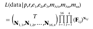
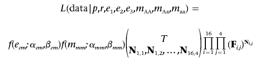
Let matrix N (not shown) be analogous to matrix F, where element N_i,j gives the observed number of trios with observed parental genotypes i and observed offspring genotype j. Let T be the total number of observed trios.

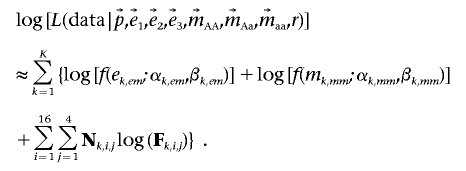
Thus, N is the “data,” and F contains our expectations for the data as a function of eight unknown parameters, p, r, e₁, e₂, e₃, m_AA, m_Aa, and m_aa, where p is the frequency of the α₁ allele; r is the frequency of the α₀ allele; e₁, e₂, and e₃ are the genotype-error rates; and m_AA, m_Aa, and m_aa are the genotype missing-data rates. In general, we assume that the elements of N are multinomially distributed with expected proportions given in the corresponding element of F. Thus, the overall likelihood of our data is given by

and

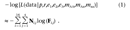Using this framework, we built two nested likelihood models. In the null model, we assumed that no deletion is present and, therefore, that r=0. The other parameters, p, e₁, e₂, e₃, m_AA, m_Aa, and m_aa, were set equal to their maximum-likelihood values found by numerically minimizing equation (1) with the use of Powell’s algorithm.⁴⁷ Under the alternate model, all eight parameters were set equal to their maximum-likelihood values. We compared the two models with a likelihood-ratio test⁴⁸ with 1 df. If, by the likelihood-ratio test, the alternate model fit significantly better than the null model, we suggested that a deletion may exist at the SNP.

For moderate frequency deletions, there is often relatively little power to distinguish a deletion of, say, 5% frequency from some combination of genotyping error and missing data in the 2%–5% range. For many SNP genotyping technologies, however, any genotyping error as large as 5% would be unlikely. Thus, to increase power, we borrowed an idea from the Bayesian approach and modified the likelihood equations to include terms that reflect our beliefs concerning the probability of observing a given error rate or missing-date rate. In general, we maintained a pure “frequentist” framework—that is, we focused on a single-point maximum in a likelihood equation rather than integrating over a posterior distribution. However, we penalized that likelihood for departing from our prior belief concerning the distribution of error and missing-data parameters.

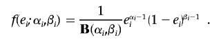
In general, we assumed that each of the three genotyping-error rates and missing-data rates are drawn from beta distributions. Thus, we assumed that error rate e_i, where 1⩽i⩽3, has probability density⁴⁹

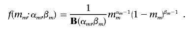
Similarly, we assumed that missing-data rate m_m, where m={AA,Aa,aa}, has probability density

Our approach is two staged. In stage one, we found the maximum-likelihood values for all eight parameters at every SNP in the study by minimizing equation (1). After all parameters were estimated, we estimated the beta-distribution parameters by the method of moments.⁵⁰ Thus, for error/missing-data parameter x, we estimated

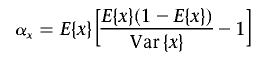and

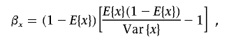where E{x} is the mean of parameter x across the SNPs, and Var{x} is the variance.

In stage two, we modified the likelihood equation to penalize for extreme error rates and missing-data rates, and we reestimated all parameters. If e_em=max{e₁,e₂,e₃} and m_mm=max{m_AA,m_Aa,m_aa}, then we penalized our likelihood to create

and

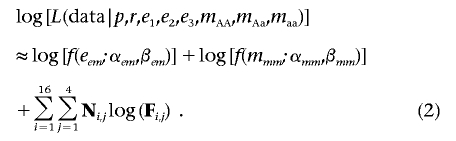In stage two, we again created two nested likelihood models by numerically minimizing equation (2), to distinguish the null from the alternate model. Once again, these models differ by one parameter, r, and can be compared by a likelihood-ratio test⁴⁸ with 1 df. If, by the likelihood-ratio test, the alternate model fit significantly better than the null model, we suggested that a deletion may exist at the SNP.

Combining Evidence between SNPs

With the above machinery, for every SNP i in the study, we estimated the probability, p_i, that the improvement in fit of the deletion model over the null model is due to chance alone with a likelihood-ratio test. Thus, 1-p_i can be thought of as the probability that SNP i is covered by a deletion independent of every other SNP in the study. Evidence was combined among SNPs in the following steps: (1) for each SNP i, with 1-p_i>0.5, we estimated who carries the putative deletion; (2) for each individual estimated to carry a deletion, we estimated the physical bounds of that deletion; (3) we combined collections of individuals with overlapping deletions into a single deletion; (4) we estimated the physical bounds of the deletion; (5) we estimated the frequency of the deletion from all the SNPs within its physical bounds; (6) given the frequency of the deletion, we reestimated the bounds; (7) we estimated a final P value for the deletion, using all the SNPs within its physical bounds; and (8) we reestimated individuals possessing the deletion, using the deletion’s entire physical bounds and estimated frequency.

(1) For each SNP i, with 1-p_i>0.5, we estimated who carries the putative deletion

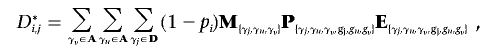
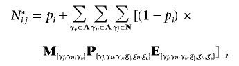
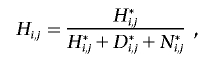
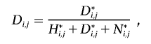
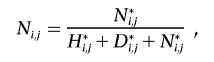
For every individual j, we wish to calculate the probability that j possesses either a heterozygous or homozygous deletion at SNP i. Let D={α₀α₀}, H={α₁α₀,α₂α₀,α₀α₁,α₀α₂}, and N={α₁α₁,α₁α₂,α₂α₁,α₂α₂} be the sets of possible homozygous deletion, heterozygous deletion, and “no deletion” genotypes, respectively. Let be the set of all possible genotypes. Let N_i,j be the probability that j’s true genotype is an element of N—that is, the probability that j possesses no deletion at SNP i. Let H_i,j and D_i,j be the respective probabilities that j is a heterozygous or homozygous deletion, where N_i,j+H_i,j+D_i,j=1. Let j’s true genotype be γ_j, and let j be part of a trio with relatives u and v, with true genotypes γ_u and γ_v and corresponding observed genotypes g_j, g_u, and g_v.

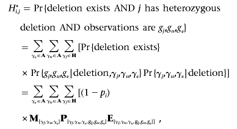and

where M_{{γj,γu,γv}}, P_{{γj,γu,γv,gj,gu,gv}}, and E_{{γj,γu,γv,gj,gu,gv}} are the elements of the true-parent/true-child, true-parent/observed-parent, and true-child/observed-child matrices, respectively, corresponding with truth {γ_j, γ_u, γ_v} and observation {g_j, g_u, g_v}. Note that j can be a homozygote for a “no deletion” either because the deletion exists but j does not possess it, or because the deletion does not exist.

(2) For each individual estimated to carry a deletion, we estimated the physical bounds of that deletion

If N_i,j<0.5 for any individual j, we have evidence that SNP i is deleted in individual j; potentially, other SNPs with weaker evidence may be deleted as well. Noting that individuals who are heterozygous or homozygous for a deletion rarely appear to be heterozygotes, since this would involve some sort of genotyping error, we assigned a putative maximum bound for individual j’s deletion by including all SNPs extending in either direction until a heterozygote was observed. We call these the maximum bounds of the deletion. Within the maximum bounds there is at least one SNP i that has positive evidence of a deletion. The minimum bounds of the deletion contain the region that includes all SNPs within the maximum that show positive evidence for a deletion (possibly just i itself).

(3) We combined collections of individuals with overlapping deletions into a single deletion

Given two overlapping deletions, a and b, occurring in different individuals, we determined whether these deletions are compatible. Let a_min and b_min represent the minimum bounds for a and b and a_max and b_max represent the maximum bounds. Two individuals were deemed to have compatible deletions if a_min was contained entirely within b_max or if b_min was contained entirely within a_max, and if a_min and b_min overlapped.

(4) We estimated the physical bounds of the deletion

We combined all compatible deletions into a “unique” deletion with physical bounds that is the minimum deletion size necessary to include the minimum region for each of the compatible deletions.

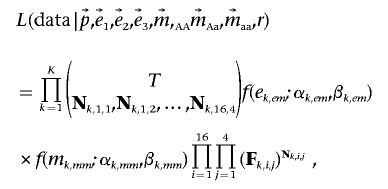
(5) We estimated the frequency of the deletion from all the SNPs within its physical bounds

For a region containing a deletion, the deletion frequency must be the same at all SNPs covered by the deletion—that is, we assumed only one segregating deletion per genomic region. For each unique deletion, we estimated r, its frequency in the population, using information from all SNPs in the deleted region. Consider a putative deletion covering K SNPs. Noting that p, e₁, e₂, e₃, m_AA, m_Aa, and m_aa vary among the K SNPs, let p, e₁, e₂, e₃, m_AA, m_Aa, and m_aa be vectors of the corresponding values across each of the K SNPs in the deleted region. The frequency of the deletion, r, on the other hand, is assumed to be a scalar and the same for all K SNPs (i.e., we assume only a single deletion within any genomic region). Thus, the likelihood of a deletion with frequency r covering all SNPs in the region is

and

(6) Given the frequency of the deletion, we reestimated the bounds

Given r, we examined SNPs adjacent to the deletion. We considered two models. In model 1, a SNP adjacent to the deletion also has a deletion with frequency r; in model 2, the deletion frequency of the adjacent SNP is 0. If model 1 fit better than model 2, we extended the deletion to this SNP and returned to step 5.

(7) We estimated a final P value for the deletion, using all the SNPs within its physical bounds

We performed a likelihood-ratio test, comparing a model with no deletion in the region with a model with a deletion with frequency r covering all the SNPs in the region. If the deletion model fit significantly better than the null model, then we inferred that a deletion spanning the entire region exists, with P value P_del taken from the likelihood-ratio test.

(8) We reestimated individuals possessing the deletion, using the deletion’s entire physical bounds and estimated frequency

For every deletion with P_del below our threshold of significance (table 2), we used the final deletion frequency r to recalculate N_i,j, H_i,j, and D_i,j for all individuals and all SNPs within the deletion. Since these values vary from SNP to SNP, we calculated an average N_j, H_j, and D_j as the harmonic mean across the SNPs:

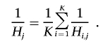We think of H_j as something like the posterior probability that individual j has a heterozygous deletion over this region. Particularly for rare and small deletions, this posterior probability may be low. However, the posterior probability might be quite high relative to the prior probability for a heterozygous deletion, which is only 2r(1-r). Thus, we considered the support for individual j having a heterozygous deletion to be H_j/2r(1-r) and the support for a homozygous deletion and no deletion to be D_j/r² and N_j/(1-r)², respectively.

Table 2. .

Threshold Matrix

	Pdela
No. of Deleted SNPs	N=30	N=100	N=500	N=1,000
1	1×10−7	1×10−6	1×10−4	1×10−4
2	1×10−8	1×10−6	1×10−5	1×10−4
3	1×10−9	1×10−7	1×10−6	1×10−5
⩾4	1×10−11	1×10−8	1×10−7	1×10−6
⩾10	1×10−15	1×10−9	1×10−7	1×10−7

^aP_del needed for significance, given a particular combination of trio size (N) and number of SNPs deleted.

Individuals are assigned genotypes by use of a four-pass process. In step (4) above, individuals with deletions “compatible” with this physical location in the genome were identified. In the first pass, these individuals are assigned a genotype if that support for the genotype is 10-fold higher than that for any other genotype. In the second pass, any individual (regardless of whether they were originally identified as having a deletion compatible with this location) is assigned a genotype if the genotype demonstrates support 20 times larger than the other two combined. With the use of these two rules, most, but not all, individuals possessing deletions are identified. Generally, the number of individuals assigned the deletion genotype in the first two passes is lower than would be implied by the frequency of the deletion. The genotype support for individuals who have not been assigned a genotype is indistinguishable. So, in the third pass, we pick parental individuals to have a deletion stochastically. We pick parent i to have a deletion with probability H_i/, where the sum is taken over all j individuals not yet assigned a genotype. Thus, the probability of being assigned a deletion is proportional to the posterior probability of having the deletion. In the third pass, parents are picked until the deletion frequency in the sample reaches the deletion frequency estimated for the population. Parents not picked in the third pass are assigned a homozygous nondeletion genotype. At this point, all parents have been assigned a genotype. In the fourth pass, the genotype support for all unassigned children is recalculated, with conditioning on the putatively known parental genotype. Children are assigned a genotype if the support for that genotype is 10 times greater than that for any other genotype. Children with weaker support are assigned genotypes stochastically, proportional to the relative support for the genotype.

Association Testing

For each deletion, every individual in the population has now been assigned one of the following genotypes: homozygous deletion, heterozygous deletion, or no deletion. Given an affected-trio study design (two parents with affected offspring), we obtained informative transmission counts for the deletion from heterozygous parents to offspring and performed a standard TDT⁴⁶ (P<.05) for the deletion. Given an affected trio combined with an unaffected trio (two parents with unaffected offspring) from a matched control group, we also performed population-based association testing. To do so, we compared the deletion frequency for affected offspring with the frequency for unaffected offspring, with a standard χ² test (P<.05).

Deletion Simulations

Genotype data were simulated using a Wright-Fisher coalescent model incorporating recombination, genotyping error, and missing data with a deletion at a given frequency placed on the coalescent. Nuclear families follow Mendelian assortment. All SNPs have a dbSNP-like minor-allele frequency.⁵¹ Each simulation consists of 250 kb of sequence with a whole-genome SNP density based on 500,000 SNPs. Error rates and missing-data rates vary by SNP, with mean and variance drawn from HapMap data.⁵² Each simulation varied given the following parameters: a combination of genotyping error and missing data rates drawn from one of eight HapMap genotyping centers (EM₁–EM₈), deletion frequency (0.5%, 1%, 5%, 10%, and 20%), deletion size (1 kb, 5 kb, 10 kb, 20 kb, and 100 kb), and number of trios in the study (30, 100, 500, and 1,000). We tested 80,000 total deletion simulations (100 for each combination of parameters). Simulated data are presented as averages over all genotyping centers (figs. 2–7).

Figure 2. .

Power to detect deletions of 5 kb (A), 10 kb (B), 20 kb (C), and 100 kb (D). SNP density is one SNP per 6 kb. Each bar represents an average with SD of 800 deletion simulations conducted for a particular trio size (i.e., 30, 100, 500, or 1,000).

Figure 3. .

Mean error number of deleted SNPs with the use of 1,000 trios, given a deletion of 5 kb (A), 10 kb (B), 20 kb (C), and 100 kb (D). Each point represents an average with SD of 800 deletion simulations.

Figure 4. .

Estimated frequencies versus true frequencies for deletions of 5 kb (A), 10 kb (B), 20 kb (C), and 100 kb (D). SNP density is one SNP per 6 kb. Each bar represents an average with SE of 800 deletion simulations conducted for a particular trio size (i.e., 30, 100, 500, or 1,000).

Figure 5. .

Sensitivity given a deletion of 5 kb (A), 10 kb (B), 20 kb (C), and 100 kb (D). SNP density is one SNP per 6 kb. Each bar represents an average with SE of 800 deletion simulations conducted for a particular trio size (i.e., 30, 100, 500, or 1,000).

Figure 6. .

Power to detect association with use of the TDT (P<.05), given a deletion of 20 kb with GRR of 1 (A), 2 (B), 3 (C), and 4 (D). GRR of 1 represents a deletion with no association. SNP density is one SNP per 6 kb. Each bar represents an average with SD of 800 deletion simulations conducted for a particular trio size (i.e., 30, 100, 500, or 1,000).

Figure 7. .

Power to detect association with the use of case-control analysis (P<.05), given a deletion of 20 kb with GRR of 1 (A), 2 (B), 3 (C), and 4 (D). GRR of 1 represents a deletion with no association. SNP density is one SNP per 6 kb. Each bar represents an average with SD of 800 deletion simulations conducted for a particular trio size (i.e., 30, 100, 500, or 1,000).

Null Simulations

Null genotype data were simulated using the same method as above, except that no deletion was placed on the coalescent. Each simulation consists of 2 Mb of sequence with a whole-genome SNP density based on 500,000 SNPs. We tested 8,000 total null simulations (1,000 for each combination of sample size and genotyping center). Data are presented as averages over all genotyping centers, yielding 2 billion bp of deletion-free sequence for each sample size.

HapMap Data

We obtained genotypes for all 22 autosomes from the unfiltered HapMap 16c phase I data set.⁵² This consisted of 866,757 SNPs from 90 CEPH individuals (30 trios) of European ancestry sampled in Utah (CEU) and 932,404 SNPs from 90 individuals (30 trios) of Yoruba ancestry sampled in Ibadan, Nigeria (YRI). For genotypes typed by more than one center, we took the consensus genotype. If a consensus did not exist, then we called the genotype “missing data,” N. We filtered the genotype data to exclude any SNP with >20% missing data or >20% genotyping error, or that exhibited a statistically significant excess of heterozygotes (F<0 and P<0.05 for Hardy-Weinberg equilibrium).⁵³

Results

We demonstrate the effectiveness of our method, using both simulated and real data. First, we establish our false-positive deletion detection rate—that is, the rate at which we infer deletions when they do not actually exist. Our overall false-positive rate for detecting a deletion is small, even at whole-genome scales. In null simulations that use 30 trios and a total of 2.66 million SNPs, we detect 34 false deletions, where the average deletion spans 2.4 SNPs (table 3). This yields a false-positive rate of 3.12×10^-5 per SNP. The false-positive rate remains consistent regardless of sample size (data not shown). From this, we expect ∼23 false deletions (totaling 56 SNPs) when applying this approach to the unfiltered HapMap 16c phase I data set.⁴³

Table 3. .

False-Positive Rate in Null Simulations

	No. of
Centera	Trios	False Deletions	Deleted SNPs	Total SNPs	FPRa per SNP
EM1	30	3	7	331,922	2.11×10−5
EM2	30	6	14	332,419	4.21×10−5
EM3	30	5	9	332,043	2.71×10−5
EM4	30	1	1	332,377	3.01×10−6
EM5	30	0	0	332,362	0
EM6	30	3	7	332,333	2.11×10−5
EM7	30	10	21	332,244	6.32×10−5
EM8	30	6	24	332,388	7.22×10−5
Total	30	34	83	2,660,000	3.12×10−5

^aEight combinations (EM₁–EM₈) of genotyping-error and missing-data rates were drawn from the eight HapMap genotyping centers. For each EM combination, 1,000 simulations were performed with ∼2 Mb of deletion-free sequence each and one SNP per 6 kb.

^bFPR = false-positive rate.

Next, we gauge our power to find deletions when they do exist. Figure 2 shows our power, in simulated data with a whole-genome SNP density of 500,000 SNPs, to detect deletions of 5 kb, 10 kb, 20 kb, and 100 kb with deletion frequencies ranging from 0.5%–20%, with the use of sample sizes of 30, 100, 500, and 1,000 trios. Power increases with increasing deletion size, deletion frequency, sample size, and SNP density. Varying genotyping-error rates and missing-data rates have little or no effect on our ability to detect deletions.

On detecting a deletion, we estimated the boundaries of the deletion (i.e., the start SNP and the stop SNP), which often included a high percentage of the SNPs in the true deletion, if not all of them (fig. 3). For rare deletions—say, 100 kb (∼16.7 SNPs deleted) at 0.5% frequency—the mean error in number of deleted SNPs is 1.8 in 1,000 trios (fig. 3). This shows that, for rare variants, we tend to be biased and to slightly underestimate the true bounds, but only by a few SNPs. As frequency increases—say, 100 kb at 20% frequency—the mean error in number of deleted SNPs is effectively unbiased (0.03). For most cases, including smaller sample sizes (data not shown), estimates of the deletion bounds are within a single SNP of the true bounds (i.e., the SD in the error estimate is usually smaller than one SNP).

Estimates of the deletion frequency are highly accurate (figure 4). Using large study designs of 1,000 trios, we are able to return extremely accurate estimates of the true frequency with percent error less than one for deletions as small as 5 kb or as rare as 1% frequency. For example, given a 100-kb deletion with true deletion frequency of 20%, we estimate the deletion frequency to be, on average, 20.01% with SD 0.0082. Estimated frequency is biased when the power to detect the deletion is very low. Thus, we suffer the classic winner’s curse. When underpowered to detect the deletion, we tend to overestimate the deletion frequency.

Even with accurate estimates of the deletion frequency, our sensitivity, or ability to identify every individual in the population who carries the deletion, is never perfect (figure 5). This is largely due to misidentifying parents with untransmitted deletions. For example, given a 100-kb deletion at frequency 5%, using a sample of 30 trios, we correctly identify 95% of parents with transmitted deletions but only 60% of parents with untransmitted deletions, which leads to an overall sensitivity of 85%.

We tested our detected deletions for association with disease. We maintain nominal false-positive rates for showing association when the deletion is unassociated with disease (genotype-relative risk [GRR] 1), and we demonstrate substantial power to show disease association when it is present (GRR >1). Power to detect association using standard TDT given a deletion with GRR of 1, 2, 3, and 4 is shown in figure 6 (a multiplicative model of disease is assumed).⁵¹ Power to detect association (P<.05) with the use of an affected-trio versus unaffected-trio case-control design with GRR of 1, 2, 3, and 4 is shown in figure 7. In 80,000 simulations with an unassociated deletion (GRR 1), over the entire range of parameter values examined, our rate for detecting and then falsely associating the deletion is 2.0% and 2.4% for the TDT and case-control designs, respectively, at nominal P<.05. However, when deletions are absent from the data, they can still be detected erroneously at the false-deletion detection rate of 3.12×10^-5 per SNP. These false deletions generally span three or fewer SNPs and tend to appear significantly undertransmitted (data not shown), especially when the deletion is more than three SNPs in length. Therefore, deletions that showed significant undertransmission from the TDT (P<.05) were excluded from our HapMap survey.

Here, we report 693 total deletions (see the tab-delimited ASCII file, which can be imported into a spreadsheet, of data set 1), with 213 deletions found in the sample of 90 CEU individuals and 480 deletions found in the sample of 90 YRI individuals. Overall, 329 (47%) deletions span multiple SNPs, 532 (77%) exist in the homozygous state, and 253 (37%) have been validated by one or more previous studies (table 4). On average, each CEU individual has 2.6 Mb deleted, whereas each YRI individual has 6.0 Mb deleted (data not shown). The distribution of length (figure 8) ranges from 1 bp to 794 kb (average 20.2 kb; median 3.6 kb) in CEU individuals and from 1 bp to 145 kb (average 5.9 kb; median 1 bp) in YRI individuals. The distribution of frequency estimates ranges from 2.7% to 47.8% (average 18.7%; median 19.2%) in CEU individuals (fig. 9A) and from 3.6% to 70.0% (average 21.6; median 20.3) in YRI individuals (fig. 9B). For all validated deletions, the sizes range from 1 bp to 794 kb (average 16.3 kb; median 3.6 kb), with estimated frequencies from 2.7% to 46.4% (average 18.6%; median 16.6%); for all novel deletions (those not previously identified by other studies), the sizes range from 1 bp to 245 kb (average 6.8 kb; median 1 bp), with estimated frequencies from 3.0% to 70.0% (average 21.9; median 20.9).

Table 4. .

Most Significant Deletions in HapMap Collection^[Note]

				No. of
Start	End	Chromosome	Size (bp)	Deleted SNPs	Heta	Homb	Deletion Frequency	Pdel	PTDT	Population	Validation
69120910	69165549	4	44,640	15	44	3	.288	9.6×10−80	.369	CEU	Conrad et al.,44 Redon et al.,29 Sharp et al.27
69130187	69165549	4	35,363	19	37	2	.221	1.8×10−79	.835	YRI	Conrad et al.,44 Redon et al.,29 Sharp et al.27
13659506	13693201	8	33,696	15	24	1	.133	9.7×10−66	.317	YRI	Conrad et al.,44 McCarroll et al.,45 Mills et al.,68 Redon et al.29
39423310	39492651	8	69,342	32	14	0	.078	4.2×10−65	.527	YRI	Conrad et al.,44 McCarroll et al.,45 Redon et al.29
34456637	34507878	4	51,242	19	20	1	.126	1.6×10−45	.109	YRI	Conrad et al.,44 Iafrate et al.,23 McCarroll et al.,45 Sebat et al.25
11398341	11434605	12	36,265	13	28	3	.208	1.7×10−44	.180	YRI	Conrad et al.,44 McCarroll et al.,45 Redon et al.29
11398341	11438799	12	40,459	13	16	1	.087	9.2×10−41	.366	CEU	Conrad et al.,44 McCarroll et al.,45 Redon et al.29
39469612	39497557	8	27,946	13	44	16	.395	6.4×10−40	.394	CEU	Conrad et al.,44 McCarroll et al.,45 Redon et al.29
25030376	25045471	8	15,096	8	25	0	.137	3.6×10−39	.808	YRI	Conrad et al.,44 McCarroll et al.,45 Redon et al.29
64380379	64392138	4	11,760	4	37	9	.321	2.3×10−36	.161	CEU	McCarroll et al.45
71425108	71495782	18	70,675	73	5	0	.043	4.9×10−35	.317	YRI	…
115392087	115401739	4	9,653	5	41	14	.376	1.8×10−34	.336	YRI	McCarroll et al.,45 Redon et al.29
61416760	61498398	7	81,639	16	25	0	.142	5.1×10−34	.346	YRI	Conrad et al.,44 Redon et al.29
27539977	27545038	12	5,062	6	22	3	.163	7.5×10−34	.796	YRI	Conrad et al.,44 McCarroll et al.,45 Redon et al.29
21247095	21299228	22	52,134	21	6	0	.040	3.2×10−33	.180	CEU	Locke et al.,28 McCarroll et al.,45 Sebat et al.25
133555158	133800547	5	245,390	50	15	0	.080	5.8×10−32	1	CEU	…
65166887	65188519	3	21,633	16	26	0	.127	1.6×10−30	.317	CEU	Conrad et al.,44 McCarroll et al.,45 Redon et al.29
71027351	71049091	18	21,741	30	6	0	.073	5.4×10−30	.180	YRI	…
23931936	24211173	10	279,238	67	15	0	.081	6.9×10−30	1	CEU	Wong et al.30
70250280	70262009	4	11,730	4	45	12	.390	1.4×10−29	.577	YRI	Conrad et al.,44 Locke et al.,28 McCarroll et al.,45 Redon et al.29
70174665	70227396	4	52,732	14	50	3	.300	3.1×10−29	.384	YRI	Conrad et al.,44 McCarroll et al.,45 Redon et al.29
109229673	109238466	7	8,794	8	26	2	.150	4.1×10−29	.491	YRI	Conrad et al.,44 McCarroll et al.,45 Tuzun et al.32
20724046	20753953	21	29,908	25	5	0	.036	1.1×10−28	.317	YRI	Conrad et al.,44 Redon et al.29
60798055	60847919	3	49,868	20	15	0	.081	5.7×10−27	.527	CEU	Conrad et al.,44 McCarroll et al.,45 Redon et al.29
104428735	104434065	4	5,331	9	18	1	.096	9.2×10−27	.248	YRI	Conrad et al.,44 McCarroll et al.,45 Redon et al.,29 Sebat et al.25
147377167	147414362	1	37,196	15	23	0	.119	3.0×10−26	.796	CEU	Conrad et al.,44 Redon et al.,29 Wong et al.30
70058756	70094563	18	35,808	44	7	0	.045	9.7×10−26	.102	YRI	…
246287577	246402642	1	115,066	27	25	0	.117	2.0×10−24	.796	CEU	Redon et al.29
241828358	241912790	1	84,433	19	7	0	.052	4.6×10−24	.655	CEU	…
21359263	21422160	22	62,898	17	11	1	.088	5.5×10−24	.157	YRI	McCarroll et al.,45 Simon-Sanchez et al.,69 Urban et al.70
164029860	164077953	3	48,094	20	44	0	.230	8.5×10−24	.450	CEU	Conrad et al.,44 McCarroll et al.,45 Redon et al.,29 Tuzun et al.,32 Wong et al.30
133425381	133446804	7	21,424	9	21	1	.122	8.5×10−24	.782	YRI	Conrad et al.,44 McCarroll et al.,45 Redon et al.29
93165059	93168493	7	3,435	4	33	4	.224	4.6×10−23	.835	CEU	Conrad et al.,44 McCarroll et al.45
41095773	41099005	2	3,233	3	34	4	.236	5.2×10−23	.513	YRI	Conrad et al.,44 McCarroll et al.45
147460714	147505129	1	44,416	16	19	0	.110	1.5×10−22	.109	CEU	Conrad et al.,44 McCarroll et al.,45 Redon et al.,29 Wong et al.30
20803641	20831833	22	28,193	12	10	0	.054	1.7×10−22	.705	CEU	McCarroll et al.,45 Simon-Sanchez et al.69
39351896	39456066	8	104,171	35	20	0	.094	1.9×10−22	1	CEU	Conrad et al.,44 McCarroll et al.,45 Redon et al.29
190846788	190850343	3	3,556	3	29	3	.187	3.8×10−22	.827	YRI	Conrad et al.,44 McCarroll et al.45
70240740	70262009	4	21,270	6	18	0	.100	4.0×10−22	.564	CEU	Conrad et al.,44 McCarroll et al.,45 Locke et al.,28 Redon et al.29
78665072	78684492	7	19,421	9	17	0	.083	4.6×10−22	.206	YRI	Conrad et al.,44 McCarroll et al.,45 Redon et al.29

Note.— Chromosome start and end positions are relative to NCBI build 36.

^aHeterozygous deletions observed.

^bHomozygous deletions observed.

Figure 8. .

Distribution of deletion size in HapMap individuals. Red indicates the number of deletions observed in YRI individuals. Blue indicates the number of deletions observed in CEU individuals. The first bin represents the number of single-SNP deletions. Every bin after that represents a distance of 5 kb. The second bin shows the number of deletions <5 kb (excluding all single-SNP deletions). The last bin shows the number of deletions >100 kb.

Figure 9. .

Distribution of frequency for 90 CEU individuals (30 trios) (A) and for 90 YRI individuals (30 trios) (B). Full color indicates the contribution from deletions of two or more SNPs. Half-shading indicates the contribution from single-SNP deletions. Every bin represents a frequency difference of 1%. The last bin shows the number of deletions with frequency >50%.

Our computational tool to detect deletions, microdel, and our deletion simulator are available for free download as C source code from the author's Web site and are licensed under the General Public License.

Discussion

It has long been recognized that CNV in general, and deletions in particular, can play an important role in the etiology of rare disorders.^4,36 Elucidating the role of CNV in common, complex disorders has proved to be difficult.^{13,14,54–56} The nature of complex disease is one of multiple factors, each usually with relatively small effect. Hence, the demonstration of association between any genetic variant, whether deletion or SNP, and a complex disorder generally requires large study designs.^51,57–60 Many techniques to study CNVs, however, are unable to detect small deletions^20,61 or are time consuming and expensive to perform on a large scale.^30,32,62

The need for large study designs and the expense of many techniques that detect deletions has led to a flurry of recent research to find methods that can detect deletions efficiently, cheaply, and, ideally, in the context of a preexisting study.^44,45 With the advent of high-density SNP arrays, large-scale whole-genome association studies have become a powerful and realistic approach in the search for genetic factors underlying complex phenotypes. Techniques aimed at identifying deletions solely from hybridization intensities may or may not be compatible with data already collected, whereas an approach that uses genotype data could easily be applied to existing SNP data sets. Developing tools and strategies that harness the information in SNP genotype data to detect deletions at high power may enable a single study to test not only for association with SNPs but also for association with deletions. To take advantage of this all-in-one design, accurate frequencies must be assigned to deletions.

This means that, for a deletion to be useful in a disease-association study, it must not only be detectable but must also be assigned an accurate estimate of either its population frequency or its transmission frequency or both. Thus, complex disease association studies fundamentally test questions of frequency. For a tool to be useful in this context, the tool must be able to detect the deletion at high power with a low false-positive rate and must also return an accurate estimate of its transmission from heterozygous parents to offspring or its occurrence in cases versus controls. The tool developed here, microdel, is the first, to our knowledge, aimed at both halves of this problem.

Our approach facilitates simultaneous discovery and testing of small segregating deletions for association with disease in large-scale familial SNP genotyping studies. Given the density of current array designs, we demonstrate the usefulness of microdel on simulated data with a whole-genome SNP density based on 500,000 SNPs. With a modestly large study design of 500 trios, microdel can detect deletions as small as 10 kb or as rare as 1% frequency with at least 80% power and, in all cases, return sufficiently accurate estimates of both population frequency and transmission frequency, for the performance of association tests on the detected deletion. Increasing the study design to 1,000 trios provides a substantial boost in microdel's power to detect very rare deletions of <1% frequency while returning extremely accurate estimates of the deletion frequency. Decreasing the study design to 100 trios still enables discovery of deletions as small as 20 kb or as rare as 5% frequency with >80% power. This illustrates the potential usefulness of microdel as a tool to not only detect deletions at high power but to also test the inferred deletion for association with disease using both case-control analysis and the TDT.

We examine two sorts of association study designs: (1) a typical TDT design (two parents and one affected offspring) and (2) a typical TDT design combined with two parents and unaffected offspring from some matched control group. We call this second design a “case trio–control trio” design, or just “case-control trio” for simplicity. In the presence of true disease association, the case-control trio design tends to be more powerful. We show in figure 4 that, under the null model of no association with disease, we accurately estimate the frequency of deletions in the general population. Under the alternate model (where disease association is present), however, we tend to overestimate the deletion frequency in the general population (data not shown). Thus, we overestimate the number of untransmitted chromosomes in the first design, leading to reduced power with use of the TDT only. By adding control trios, even in the presence of disease, the deletion frequency is better estimated, and power increases.

Other methods, both computational and experimental, exist to detect CNV; however, there is no consensus approach to identify all types of variants, as evidenced by the little overlap seen in previous studies (Database of Genomic Variants). Here, we report 440 novel variants in the HapMap collection with an estimated false-positive rate of ∼5%, whereas the remaining 253 deletions have been validated by one or more previous studies (Database of Genomic Variants). Not surprisingly, our survey shows considerable overlap with the computational approaches of Conrad et al.⁴⁴ and McCarroll et al.,⁴⁵ both jointly and individually (table 4). In instances where we fail to report deletions found by both Conrad et al.⁴⁴ and McCarroll et al.,⁴⁵ we usually have evidence that a deletion may exist, but the P value for the deletion falls just above our threshold of significance (see the tab-delimited ASCII file of data set 2). More notably, microdel is capable of inferring deletions that are reported by noncomputational techniques, such as the fine-scale fosmid-based approach used by Tuzun et al.³² and recent array-based studies conducted by Redon et al.²⁹ and Wong et al.³⁰ (table 4), but that are missed by other computational approaches.^44,45

Our framework for finding a deletion compares a model with a deletion with a model without a deletion and infers the presence of the deletion when the deletion model fits much better than the null model. It is also possible that neither model describes the truth very well and that there is some third, unconsidered alternative explanation that fits the data. For example, it has been shown that genotyping studies with the use of DNA from cell lines may contain somatic cell–line artifacts that appear as deletions.^29,44 Given the level of statistical evidence needed for our method to detect a deletion, it is unlikely we would detect cell-line artifacts unless they are of substantial size or occur in multiple individuals. Therefore, large, unvalidated deletions in our survey of HapMap individuals may be cell-line artifacts, but this number is small, since only five deletions >100 kb in size were invalidated. Second, SNP genotype assays rely on techniques (e.g., restriction digests and primer hybridization) that are sensitive to cryptic polymorphisms. Single-SNP aberrations may result when one allele is ineffectively assayed because of a cryptic SNP residing in a location crucial to the success of the assay (i.e., a restriction-enzyme cutting site or the genomic sequence targeted for primer hybridization). Thus, single-SNP deletions in our HapMap survey may potentially be the result of nearby cryptic SNPs, which in and of themselves are worth noting, whereas others are undoubtedly real deletions, since 82 of our 364 reported single-SNP deletions were shown to occur in previously reported regions of variation (Database of Genomic Variants).

The approach taken by microdel, as well as the computational tools of Conrad et al.⁴⁴ and McCarroll et al.,⁴⁵ fundamentally uses only a fraction of the information available from modern whole-genome microarrays. In particular, we use only the actual genotype call and do nothing with the relative hybridization intensity. Since other techniques exist to infer deletions from the hybridization intensity^29,63–67 without use of the genotype call per se, it seems natural that the ultimate approach to these sorts of studies will combine both types of data into a single framework.

References

- 1.Jacobs PA, Baikie AG, Court Brown WM, Strong JA (1959) The somatic chromosomes in mongolism. Lancet 1:710 10.1016/S0140-6736(59)91892-6 [DOI] [PubMed] [Google Scholar]
- 2.Edwards JH, Harnden DG, Cameron AH, Crosse VM, Wolff OH (1960) A new trisomic syndrome. Lancet 1:787–790 10.1016/S0140-6736(60)90675-9 [DOI] [PubMed] [Google Scholar]
- 3.Lupski JR, de Oca-Luna RM, Slaugenhaupt S, Pentao L, Guzzetta V, Trask BJ, Saucedo-Cardenas O, Barker DF, Killian JM, Garcia CA, et al (1991) DNA duplication associated with Charcot-Marie-Tooth disease type 1A. Cell 66:219–232 10.1016/0092-8674(91)90613-4 [DOI] [PubMed] [Google Scholar]
- 4.Carlson C, Sirotkin H, Pandita R, Goldberg R, McKie J, Wadey R, Patanjali SR, Weissman SM, Anyane-Yeboa K, Warburton D, et al (1997) Molecular definition of 22q11 deletions in 151 velo-cardio-facial syndrome patients. Am J Hum Genet 61:620–629 [DOI] [PMC free article] [PubMed] [Google Scholar]
- 5.Inoue K, Lupski JR (2002) Molecular mechanisms for genomic disorders. Annu Rev Genomics Hum Genet 3:199–242 10.1146/annurev.genom.3.032802.120023 [DOI] [PubMed] [Google Scholar]
- 6.Lee JA, Lupski JR (2006) Genomic rearrangements and gene copy-number alterations as a cause of nervous system disorders. Neuron 52:103–121 10.1016/j.neuron.2006.09.027 [DOI] [PubMed] [Google Scholar]
- 7.Hollox EJ, Armour JA, Barber JC (2003) Extensive normal copy number variation of a β-defensin antimicrobial-gene cluster. Am J Hum Genet 73:591–600 [DOI] [PMC free article] [PubMed] [Google Scholar]
- 8.Gonzalez E, Kulkarni H, Bolivar H, Mangano A, Sanchez R, Catano G, Nibbs RJ, Freedman BI, Quinones MP, Bamshad MJ, et al (2005) The influence of CCL3L1 gene-containing segmental duplications on HIV-1/AIDS susceptibility. Science 307:1434–1440 10.1126/science.1101160 [DOI] [PubMed] [Google Scholar]
- 9.Ledesma MC, Agundez JA (2005) Identification of subtypes of CYP2D gene rearrangements among carriers of CYP2D6 gene deletion and duplication. Clin Chem 51:939–943 10.1373/clinchem.2004.046326 [DOI] [PubMed] [Google Scholar]
- 10.Ouahchi K, Lindeman N, Lee C (2006) Copy number variants and pharmacogenomics. Pharmacogenomics 7:25–29 10.2217/14622416.7.1.25 [DOI] [PubMed] [Google Scholar]
- 11.Aitman TJ, Dong R, Vyse TJ, Norsworthy PJ, Johnson MD, Smith J, Mangion J, Roberton-Lowe C, Marshall AJ, Petretto E, et al (2006) Copy number polymorphism in Fcgr3 predisposes to glomerulonephritis in rats and humans. Nature 439:851–855 10.1038/nature04489 [DOI] [PubMed] [Google Scholar]
- 12.Buckland PR (2003) Polymorphically duplicated genes: their relevance to phenotypic variation in humans. Ann Med 35:308–315 10.1080/07853890310001276 [DOI] [PubMed] [Google Scholar]
- 13.Feuk L, Marshall CR, Wintle RF, Scherer SW (2006) Structural variants: changing the landscape of chromosomes and design of disease studies. Hum Mol Genet 15:R57–R66 10.1093/hmg/ddl057 [DOI] [PubMed] [Google Scholar]
- 14.Freeman JL, Perry GH, Feuk L, Redon R, McCarroll SA, Altshuler DM, Aburatani H, Jones KW, Tyler-Smith C, Hurles ME, et al (2006) Copy number variation: new insights in genome diversity. Genome Res 16:949–961 10.1101/gr.3677206 [DOI] [PubMed] [Google Scholar]
- 15.Jacobs PA, Matsuura JS, Mayer M, Newlands IM (1978) A cytogenetic survey of an institution for the mentally retarded. I. Chromosome abnormalities. Clin Genet 13:37–60 [DOI] [PubMed] [Google Scholar]
- 16.Coco R, Penchaszadeh VB (1982) Cytogenetic findings in 200 children with mental retardation and multiple congenital anomalies of unknown cause. Am J Med Genet 12:155–173 10.1002/ajmg.1320120206 [DOI] [PubMed] [Google Scholar]
- 17.de Vries BB, Pfundt R, Leisink M, Koolen DA, Vissers LE, Janssen IM, Reijmersdal S, Nillesen WM, Huys EH, Leeuw N, et al (2005) Diagnostic genome profiling in mental retardation. Am J Hum Genet 77:606–616 [DOI] [PMC free article] [PubMed] [Google Scholar]
- 18.Shaw-Smith C, Redon R, Rickman L, Rio M, Willatt L, Fiegler H, Firth H, Sanlaville D, Winter R, Colleaux L, et al (2004) Microarray based comparative genomic hybridisation (array-CGH) detects submicroscopic chromosomal deletions and duplications in patients with learning disability/mental retardation and dysmorphic features. J Med Genet 41:241–248 10.1136/jmg.2003.017731 [DOI] [PMC free article] [PubMed] [Google Scholar]
- 19.Vissers LE, Veltman JA, van Kessel AG, Brunner HG (2005) Identification of disease genes by whole genome CGH arrays. Hum Mol Genet 14:R215–R223 10.1093/hmg/ddi268 [DOI] [PubMed] [Google Scholar]
- 20.Kallioniemi A, Kallioniemi OP, Sudar D, Rutovitz D, Gray JW, Waldman F, Pinkel D (1992) Comparative genomic hybridization for molecular cytogenetic analysis of solid tumors. Science 258:818–821 10.1126/science.1359641 [DOI] [PubMed] [Google Scholar]
- 21.Solinas-Toldo S, Lampel S, Stilgenbauer S, Nickolenko J, Benner A, Dohner H, Cremer T, Lichter P (1997) Matrix-based comparative genomic hybridization: biochips to screen for genomic imbalances. Genes Chromosomes Cancer 20:399–407 [DOI] [PubMed] [Google Scholar]
- 22.Feuk L, Carson AR, Scherer SW (2006) Structural variation in the human genome. Nat Rev Genet 7:85–97 10.1038/nrg1767 [DOI] [PubMed] [Google Scholar]
- 23.Iafrate AJ, Feuk L, Rivera MN, Listewnik ML, Donahoe PK, Qi Y, Scherer SW, Lee C (2004) Detection of large-scale variation in the human genome. Nat Genet 36:949–951 10.1038/ng1416 [DOI] [PubMed] [Google Scholar]
- 24.Lucito R, Healy J, Alexander J, Reiner A, Esposito D, Chi M, Rodgers L, Brady A, Sebat J, Troge J, et al (2003) Representational oligonucleotide microarray analysis: a high-resolution method to detect genome copy number variation. Genome Res 13:2291–2305 10.1101/gr.1349003 [DOI] [PMC free article] [PubMed] [Google Scholar]
- 25.Sebat J, Lakshmi B, Troge J, Alexander J, Young J, Lundin P, Maner S, Massa H, Walker M, Chi M, et al (2004) Large-scale copy number polymorphism in the human genome. Science 305:525–528 10.1126/science.1098918 [DOI] [PubMed] [Google Scholar]
- 26.Bailey JA, Yavor AM, Massa HF, Trask BJ, Eichler EE (2001) Segmental duplications: organization and impact within the current human genome project assembly. Genome Res 11:1005–1017 10.1101/gr.GR-1871R [DOI] [PMC free article] [PubMed] [Google Scholar]
- 27.Sharp AJ, Locke DP, McGrath SD, Cheng Z, Bailey JA, Vallente RU, Pertz LM, Clark RA, Schwartz S, Segraves R, et al (2005) Segmental duplications and copy-number variation in the human genome. Am J Hum Genet 77:78–88 [DOI] [PMC free article] [PubMed] [Google Scholar]
- 28.Locke DP, Sharp AJ, McCarroll SA, McGrath SD, Newman TL, Cheng Z, Schwartz S, Albertson DG, Pinkel D, Altshuler DM, et al (2006) Linkage disequilibrium and heritability of copy-number polymorphisms within duplicated regions of the human genome. Am J Hum Genet 79:275–290 [DOI] [PMC free article] [PubMed] [Google Scholar]
- 29.Redon R, Ishikawa S, Fitch KR, Feuk L, Perry GH, Andrews TD, Fiegler H, Shapero MH, Carson AR, Chen W, et al (2006) Global variation in copy number in the human genome. Nature 444:444–454 10.1038/nature05329 [DOI] [PMC free article] [PubMed] [Google Scholar]
- 30.Wong KK, deLeeuw RJ, Dosanjh NS, Kimm LR, Cheng Z, Horsman DE, MacAulay C, Ng RT, Brown CJ, Eichler EE, et al (2007) A comprehensive analysis of common copy-number variations in the human genome. Am J Hum Genet 80:91–104 [DOI] [PMC free article] [PubMed] [Google Scholar]
- 31.Wang TL, Maierhofer C, Speicher MR, Lengauer C, Vogelstein B, Kinzler KW, Velculescu VE (2002) Digital karyotyping. Proc Natl Acad Sci USA 99:16156–16161 10.1073/pnas.202610899 [DOI] [PMC free article] [PubMed] [Google Scholar]
- 32.Tuzun E, Sharp AJ, Bailey JA, Kaul R, Morrison VA, Pertz LM, Haugen E, Hayden H, Albertson D, Pinkel D, et al (2005) Fine-scale structural variation of the human genome. Nat Genet 37:727–732 10.1038/ng1562 [DOI] [PubMed] [Google Scholar]
- 33.Matsuzaki H, Dong S, Loi H, Di X, Liu G, Hubbell E, Law J, Berntsen T, Chadha M, Hui H, et al (2004) Genotyping over 100,000 SNPs on a pair of oligonucleotide arrays. Nat Methods 1:109–111 10.1038/nmeth718 [DOI] [PubMed] [Google Scholar]
- 34.Gunderson KL, Steemers FJ, Lee G, Mendoza LG, Chee MS (2005) A genome-wide scalable SNP genotyping assay using microarray technology. Nat Genet 37:549–554 10.1038/ng1547 [DOI] [PubMed] [Google Scholar]
- 35.Steemers FJ, Chang W, Lee G, Barker DL, Shen R, Gunderson KL (2006) Whole-genome genotyping with the single-base extension assay. Nat Methods 3:31–33 10.1038/nmeth842 [DOI] [PubMed] [Google Scholar]
- 36.Chance PF, Alderson MK, Leppig KA, Lensch MW, Matsunami N, Smith B, Swanson PD, Odelberg SJ, Disteche CM, Bird TD (1993) DNA deletion associated with hereditary neuropathy with liability to pressure palsies. Cell 72:143–151 10.1016/0092-8674(93)90058-X [DOI] [PubMed] [Google Scholar]
- 37.Daiger SP, Chakravarti A (1983) Deletion mapping of polymorphic loci by apparent parental exclusion. Am J Med Genet 14:43–48 10.1002/ajmg.1320140108 [DOI] [PubMed] [Google Scholar]
- 38.Ferguson-Smith MA, Newman BF, Ellis PM, Thomson DM, Riley ID (1973) Assignment by deletion of human red cell acid phosphatase gene locus to the short arm of chromosome 2. Nat New Biol 243:271–274 10.1038/243271a0 [DOI] [PubMed] [Google Scholar]
- 39.Hirschfeld L, Hirschfeld H (1919) Serological differences between the blood of different races. Lancet 11:675–679 10.1016/S0140-6736(01)48686-7 [DOI] [Google Scholar]
- 40.Mitchell AA, Cutler DJ, Chakravarti A (2003) Undetected genotyping errors cause apparent overtransmission of common alleles in the transmission/disequilibrium test. Am J Hum Genet 72:598–610 [DOI] [PMC free article] [PubMed] [Google Scholar]
- 41.Sobel E, Papp JC, Lange K (2002) Detection and integration of genotyping errors in statistical genetics. Am J Hum Genet 70:496–508 [DOI] [PMC free article] [PubMed] [Google Scholar]
- 42.Pompanon F, Bonin A, Bellemain E, Taberlet P (2005) Genotyping errors: causes, consequences and solutions. Nat Rev Genet 6:847–859 10.1038/nrg1707 [DOI] [PubMed] [Google Scholar]
- 43.Abecasis GR, Cherny SS, Cardon LR (2001) The impact of genotyping error on family-based analysis of quantitative traits. Eur J Hum Genet 9:130–134 10.1038/sj.ejhg.5200594 [DOI] [PubMed] [Google Scholar]
- 44.Conrad DF, Andrews TD, Carter NP, Hurles ME, Pritchard JK (2006) A high-resolution survey of deletion polymorphism in the human genome. Nat Genet 38:75–81 10.1038/ng1697 [DOI] [PubMed] [Google Scholar]
- 45.McCarroll SA, Hadnott TN, Perry GH, Sabeti PC, Zody MC, Barrett JC, Dallaire S, Gabriel SB, Lee C, Daly MJ, et al (2006) Common deletion polymorphisms in the human genome. Nat Genet 38:86–92 10.1038/ng1696 [DOI] [PubMed] [Google Scholar]
- 46.Spielman RS, McGinnis RE, Ewens WJ (1993) Transmission test for linkage disequilibrium: the insulin gene region and insulin-dependent diabetes mellitus (IDDM). Am J Hum Genet 52:506–516 [PMC free article] [PubMed] [Google Scholar]
- 47.Press WH, Flannery BP, Teukolsky S, Vetterling WT(1992) Numerical recipes in C: the art of scientific computing. Cambridge University Press, Cambridge, United Kingdom [Google Scholar]
- 48.Edwards AWF (1992) Likelihood. Johns Hopkins University Press, Baltimore [Google Scholar]
- 49.Abramowitz M, Stegun IA, Knovel (1972) Handbook of mathematical functions with formulas, graphs, and mathematical tables. U.S. Department of Commerce, U.S. Government Printing Office, Washington, D.C. [Google Scholar]
- 50.Johnson NL, Kotz S, Balakrishnan N (1994) Continuous univariate distributions. Wiley and Sons, New York [Google Scholar]
- 51.Lin S, Chakravarti A, Cutler DJ (2004) Exhaustive allelic transmission disequilibrium tests as a new approach to genome-wide association studies. Nat Genet 36:1181–1188 10.1038/ng1457 [DOI] [PubMed] [Google Scholar]
- 52.International HapMap Consortium (2005) A haplotype map of the human genome. Nature 437:1299–1320 10.1038/nature04226 [DOI] [PMC free article] [PubMed] [Google Scholar]
- 53.Weir BS (1996) Genetic data analysis II : methods for discrete population genetic data. Sinauer Associates, Sunderland, MA [DOI] [PubMed] [Google Scholar]
- 54.Stranger BE, Forrest MS, Dunning M, Ingle CE, Beazley C, Thorne N, Redon R, Bird CP, de Grassi A, Lee C, et al (2007) Relative impact of nucleotide and copy number variation on gene expression phenotypes. Science 315:848–853 10.1126/science.1136678 [DOI] [PMC free article] [PubMed] [Google Scholar]
- 55.Autism Genome Project Consortium, Szatmari P, Paterson AD, Zwaigenbaum L, Roberts W, Brian J, Liu XQ, Vincent JB, Skaug JL, Thompson AP, et al (2007) Mapping autism risk loci using genetic linkage and chromosomal rearrangements. Nat Genet 39:319–328 10.1038/ng1985 [DOI] [PMC free article] [PubMed] [Google Scholar]
- 56.Sebat J, Lakshmi B, Malhotra D, Troge J, Lese-Martin C, Walsh T, Yamrom B, Yoon S, Krasnitz A, Kendall J, et al (2007) Strong association of de novo copy number mutations with autism. Science 316:445–449 10.1126/science.1138659 [DOI] [PMC free article] [PubMed] [Google Scholar]
- 57.Altshuler D, Hirschhorn JN, Klannemark M, Lindgren CM, Vohl MC, Nemesh J, Lane CR, Schaffner SF, Bolk S, Brewer C, et al (2000) The common PPARgamma Pro12Ala polymorphism is associated with decreased risk of type 2 diabetes. Nat Genet 26:76–80 10.1038/79839 [DOI] [PubMed] [Google Scholar]
- 58.Barratt BJ, Payne F, Lowe CE, Hermann R, Healy BC, Harold D, Concannon P, Gharani N, McCarthy MI, Olavesen MG, et al (2004) Remapping the insulin gene/IDDM2 locus in type 1 diabetes. Diabetes 53:1884–1889 10.2337/diabetes.53.7.1884 [DOI] [PubMed] [Google Scholar]
- 59.Hirschhorn JN, Daly MJ (2005) Genome-wide association studies for common diseases and complex traits. Nat Rev Genet 6:95–108 10.1038/nrg1521 [DOI] [PubMed] [Google Scholar]
- 60.Arking DE, Pfeufer A, Post W, Kao WH, Newton-Cheh C, Ikeda M, West K, Kashuk C, Akyol M, Perz S, et al (2006) A common genetic variant in the NOS1 regulator NOS1AP modulates cardiac repolarization. Nat Genet 38:644–651 10.1038/ng1790 [DOI] [PubMed] [Google Scholar]
- 61.Seabright M (1971) A rapid banding technique for human chromosomes. Lancet 2:971–972 10.1016/S0140-6736(71)90287-X [DOI] [PubMed] [Google Scholar]
- 62.Ishkanian AS, Malloff CA, Watson SK, DeLeeuw RJ, Chi B, Coe BP, Snijders A, Albertson DG, Pinkel D, Marra MA, et al (2004) A tiling resolution DNA microarray with complete coverage of the human genome. Nat Genet 36:299–303 10.1038/ng1307 [DOI] [PubMed] [Google Scholar]
- 63.Li C, Hung Wong W (2001) Model-based analysis of oligonucleotide arrays: model validation, design issues and standard error application. Genome Biol 2:RESEARCH0032 [DOI] [PMC free article] [PubMed] [Google Scholar]
- 64.Bignell GR, Huang J, Greshock J, Watt S, Butler A, West S, Grigorova M, Jones KW, Wei W, Stratton MR, et al (2004) High-resolution analysis of DNA copy number using oligonucleotide microarrays. Genome Res 14:287–295 10.1101/gr.2012304 [DOI] [PMC free article] [PubMed] [Google Scholar]
- 65.Huang J, Wei W, Zhang J, Liu G, Bignell GR, Stratton MR, Futreal PA, Wooster R, Jones KW, Shapero MH (2004) Whole genome DNA copy number changes identified by high density oligonucleotide arrays. Hum Genomics 1:287–299 [DOI] [PMC free article] [PubMed] [Google Scholar]
- 66.Nannya Y, Sanada M, Nakazaki K, Hosoya N, Wang L, Hangaishi A, Kurokawa M, Chiba S, Bailey DK, Kennedy GC, et al (2005) A robust algorithm for copy number detection using high-density oligonucleotide single nucleotide polymorphism genotyping arrays. Cancer Res 65:6071–6079 10.1158/0008-5472.CAN-05-0465 [DOI] [PubMed] [Google Scholar]
- 67.Komura D, Shen F, Ishikawa S, Fitch KR, Chen W, Zhang J, Liu G, Ihara S, Nakamura H, Hurles ME, et al (2006) Genome-wide detection of human copy number variations using high-density DNA oligonucleotide arrays. Genome Res 16:1575–1584 10.1101/gr.5629106 [DOI] [PMC free article] [PubMed] [Google Scholar]
- 68.Mills RE, Luttig CT, Larkins CE, Beauchamp A, Tsui C, Pittard WS, Devine SE (2006) An initial map of insertion and deletion (INDEL) variation in the human genome. Genome Res 16:1182–1190 10.1101/gr.4565806 [DOI] [PMC free article] [PubMed] [Google Scholar]
- 69.Simon-Sanchez J, Scholz S, Fung HC, Matarin M, Hernandez D, Gibbs JR, Britton A, de Vrieze FW, Peckham E, Gwinn-Hardy K, et al (2007) Genome-wide SNP assay reveals structural genomic variation, extended homozygosity and cell-line induced alterations in normal individuals. Hum Mol Genet 16:1–14 10.1093/hmg/ddl436 [DOI] [PubMed] [Google Scholar]
- 70.Urban AE, Korbel JO, Selzer R, Richmond T, Hacker A, Popescu GV, Cubells JF, Green R, Emanuel BS, Gerstein MB, et al (2006) High-resolution mapping of DNA copy alterations in human chromosome 22 using high-density tiling oligonucleotide arrays. Proc Natl Acad Sci USA 103:4534–4539 10.1073/pnas.0511340103 [DOI] [PMC free article] [PubMed] [Google Scholar]
Associated Data
This section collects any data citations, data availability statements, or supplementary materials included in this article.