

Abstract
In this paper, we propose a novel approach for cortical mapping that computes a direct map between two cortical surfaces while satisfying constraints on sulcal landmark curves. By computing the map directly, we can avoid conventional intermediate parameterizations and help simplify the cortical mapping process. The direct map in our method is formulated as the minimizer of a flexible variational energy under landmark constraints. The energy can include both a harmonic term to ensure smoothness of the map and general data terms for the matching of geometric features. Starting from a properly designed initial map, we compute the map iteratively by solving a partial differential equation (PDE) defined on the source cortical surface. For numerical implementation, a set of adaptive numerical schemes are developed to extend the technique of solving PDEs on implicit surfaces such that landmark constraints are enforced. In our experiments, we show the flexibility of the direct mapping approach by computing smooth maps following landmark constraints from two different energies. We also quantitatively compare the metric preserving property of the direct mapping method with a parametric mapping method on a group of 30 subjects. Finally, we demonstrate the direct mapping method in the brain mapping applications of atlas construction and variability analysis.
Keywords: Brain mapping, cortex, atlas, direct mapping, harmonic mapping, level-set, PDEs
1 Introduction
The cerebral cortex is a convoluted sheet of gray matter in the brain that contains many distinct areas controlling various neural functions. The size, shape, and relative locations of these areas can be affected profoundly by many normal and pathological processes. The analysis of the correlation between such structural changes and the correspondingly affected functions on the cortex is a fundamental problem in brain mapping (Welker, 1990). For such studies, cortical mapping is an important tool that can provide a detailed comparison of corresponding functional and anatomical regions on different cortices. A detailed map for a group of cortices forms the foundation for further statistical analyses of associated properties such as gray matter thickness growth or decay at specific locations on the cortex. Mapping a group of cortices to a cortical atlas also provides a valuable platform for the visualization and analysis of experimental data collected from group members.
Due to the convoluted nature and variability among different brains, mapping of the cortical surfaces poses many numerical challenges for classical surface matching algorithms such as the iterative closest point(ICP) method (Besl and McKay, 1992) and its extension in brain mapping (Wang et al., 2000). Thus, the cortical mapping problem is conventionally solved through an indirect approach as illustrated in Fig. 1. A core step in this indirect approach is the parameterization of the cortical surface that assigns a 2D coordinate to each point on the surface. Popular parameterization choices include the flat 2D plane and sphere. Considerable work has been done in this area (Schwartz and Merker, 1986; Schwartz et al., 1989; Carman et al., 1995; Drury et al., 1996; Sereno et al., 1996; Thompson and Toga, 1996; Hurdal et al., 1999; Hurdal and Stephenson, 2004; Angenent et al., 1999; Fischl et al., 1999a; Timsari and Leahy., 2000; Grossman et al., 2002; Gu et al., 2004; Tosun et al., 2004; Tosun and Prince, 2005; Ju et al., 2004; Joshi et al., 2004; Wang et al., 2005b; Van Essen, 2005). The work in (Clouchoux et al., 2005) also proposed to construct a spherical coordinate system directly on the cortical surface. In order to map a cortical surface to a flat plane, artificial cuts have to be introduced carefully to open the surface (Fischl et al., 1999a). Instead, the mapping of the cortical surface to a sphere maintains the original topology and can be automated completely.
Fig. 1.
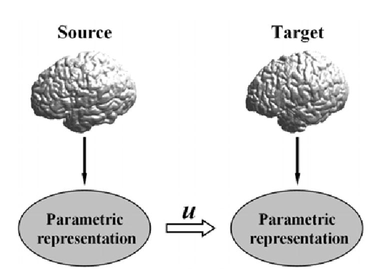
The parametric approach of cortical mapping.
Anatomical features from two different cortices however may not be parameterized with the same coordinates. To establish the final correspondences from the source cortex to the target cortex, a warping process needs to be applied in the parameterization domain under anatomically meaningful constraints. Thanks to the parameterization step, this warping process can be computed using algorithms developed in nonlinear image registration (Christensen et al., 1996; Davatzikos et al., 1996; Dupuis et al., 1998; Grenander and Miller, 1998; Toga, 1998; Joshi and Miller, 2000; Thompson et al., 2000a,b; Toga and Thompson, 2003a,b; Thompson et al., 2004; Avants and Gee, 2004). In terms of anatomical constraints in the warping process, one of the most popular choices is to constrain the map to match sulcal and gyral landmarks on both cortical surfaces (Van Essen et al., 1998; Glaunes et al., 2004; Thompson et al., 2000a,b, 2004). It is interesting to point out that sulcal landmarks were also used in many nonlinear image registration algorithms (Collins et al., 1998; Cachier et al., 2001; Hellier and Barillot, 2003). One can also apply curvature related geometric properties of the cortical surface to guide the mapping procedure (Fischl et al., 1999b; Tosun and Prince, 2005). To establish the final cortex to cortex map, the map computed in the warping process can be pulled back to both the source and target cortical surfaces using the parameterization.
In this paper, we propose a novel and PDE-based approach to compute a direct map from the source to the target cortical surface that follows constraints on sulcal landmark curves. By computing the map directly, we can simplify the whole mapping process and potentially help reduce numerical artifacts in the intermediate parameterization steps. Our work is built upon the implicit harmonic mapping method proposed in (Bertalmío et al., 2001; Mémoli et al., 2004a), which computes a map between two surfaces by iteratively solving a PDE derived from the Euler-Lagrange equation of the harmonic energy. A key step in this implicit mapping method, which is defined on the source surface, is to represent both the source and target surfaces as the zero level set of functions (Osher and Sethian, 1988), which enables the calculation of intrinsic gradients on the surfaces using well understood numerical schemes on regular Cartesian grids. The work in (Mémoli et al., 2004a), however, mainly concerns with mapping between general manifolds and no landmark constraints are considered, which is critical for our problem. The direct cortical mapping algorithm we develop here extends the work of (Mémoli et al., 2004a) in several ways. First of all, we develop a general approach to incorporate boundary conditions into implicit mapping methods. To achieve that, we construct a triangular mesh representation of the boundary condition defined on landmark curves. This makes the information of the boundary condition easily accessible on the Cartesian grid and leads us to design a set of adaptive numerical schemes to solve the PDE derived from the Euler-Lagrange equation of the harmonic energy. This enables our algorithm to minimize the harmonic energy while respecting the boundary condition. Another important element of our algorithm is a novel approach to finding an initial map between two cortical surfaces using a new feature called landmark context we develop here. This provides a reasonably good starting point for our iterative algorithm. Besides landmark constraints, we have also extended the harmonic energy with general data terms that are valuable in matching geometric features, such as the mean curvature, of the source and target cortical surface.
Recently an important result from (Mémoli et al., 2006) also considered incorporating boundary conditions into the direct mapping process. They formulated the boundary condition as defined on a set of discrete points and proposed to compute the map by minimizing its global Lipschitz constant. In contrast to the implicit approach, this method is not based on solving PDEs and finds the map using a search strategy with the aim of minimizing the Lipschitz constant. This is, in principle, a very general method, but sulcal landmarks were not tested in (Mémoli et al., 2006), so its application in cortical mapping still needs to be further studied.
In the rest of the paper, we first review the mathematical background of solving PDEs on implicit surfaces in section 2. We then propose a general variational framework for direct mapping in section 3 and extend the technique reviewed in section 2 to incorporate boundary conditions defined on landmark curves. In section 4, we develop a front propagation type method to construct initial maps based on a new feature landmark context. This provides a good starting point for our iterative algorithm. An extension of the variational energy to include general data terms is proposed in section 5. Experimental results are presented in section 6 to demonstrate our direct mapping method. Finally, conclusions are made in section 7.
2 PDEs on Implicit Surfaces
The idea of using implicit level-set representations to solve PDEs on manifolds was first introduced in (Bertalmío et al., 2001). Since our current focus is cortical mapping, we limit our discussion to surfaces embedded in , but the general idea of solving PDEs on implicit manifolds is applicable to arbitrary dimensions.
Let ℳ denote a surface and a level-set function be its implicit representation such that ℳ is the zero level set of ϕ. Though there are no particular requirement on the level-set function ϕ, we choose ϕ as the signed distance function of ℳ. This is a desirable choice since it can greatly simplify many of our mathematical derivations using the property that ∣∇ϕ∣ = 1 for a signed distance function.
To present the idea of PDEs on implicit surfaces, we use the heat diffusion equation as an example:
| (1) |
where is a function defined on the surface, and is the Laplace-Beltrami operator on ℳ, which is the intrinsic counterpart on the manifold of the Laplacian operator in Euclidean space. From a variational point of view, the equation in (1) is the flow that minimizes the harmonic energy function E defined on ℳ:
| (2) |
where is the intrinsic gradient of u on ℳ.
One of the major advantages of using the level-set representation is that all computations are performed on Cartesian grids with easy to implement numerical schemes. Besides representing the surface ℳ implicitly with a signed distance function defined on a regular grid, we also need to extend the function u off the surface to the grid so that all computations can be done implicitly. Since we only care about the solution of u on the surface, it is only necessary to extend u to a tubular narrow band around ℳ as we illustrate in Fig. 2. Typically we extend u to this narrow band such that , i.e., u is constant along the normal direction of ℳ. Numerically this can be achieved by using the fast marching method (Tsitsiklis, 1995; Sethian, 1996) or solving the following PDE in the narrow band as proposed in (Chen et al., 1997):
Fig. 2. An illustration of the narrow band of a manifold ℳ in 2D.
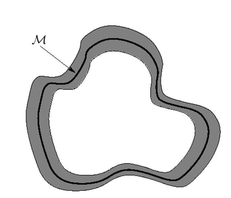
The thick curve is the manifold of interest and the gray region surrounding it is where the implicit mapping approach solve the PDE derived from the Euler-Lagrange equation of the harmonic energy.
| (3) |
After extending u to the narrow band, we can transform the energy function on ℳ into an integral over the Euclidean space. First we can represent the intrinsic gradient of u on ℳ using its implicit representation as:
| (4) |
where ∏∇ϕ is a projection operator defined as:
| (5) |
Here I is the identity operator and ∇ϕ is the normal vector of ℳ using the fact that ϕ is the signed distance function of ℳ. When we apply ∏∇ϕ to the regular gradient of u in Euclidean space, it projects ∇u onto the tangent space of ℳ. Using this projection operator, the harmonic energy in (2) can be translated into an integral over the whole Euclidean space in terms of the level-set function ϕ as:
| (6) |
We can then compute the first variation of the energy with respect to u and derive the gradient descent flow of u as in (Bertalmío et al., 2001):
| (7) |
This is the implicit form of the PDE in (1). Compared with techniques that solve the PDE explicitly on the surface, the implicit form enables us to perform all computations on the Cartesian grid and apply standard numerical schemes with well understood error measures. Since the computations are only done in a narrow band of the surface, the computational cost is on the same order as methods using explicit representations.
Besides the heat diffusion equation, a solution of fourth order PDEs on implicit surfaces is developed in (Greer et al., 2005). Also a modified projection operator for the diffusion equation is proposed in (Greer, 2005) to replace the procedure of reinitialization that extends the function u off the surface periodically. Finite element schemes are also proposed in (Burger, 2005) for the solution of PDEs on implicitly represented surfaces. Closely related to the level-set approach, a phase-field method of solving PDEs on implicit surfaces is proposed in (Ratz and Voigt, 2005).
The idea of solving PDEs on implicit surfaces is generalized to the mapping between manifolds in (Mémoli et al., 2004a,b). Assume we have a source manifold ℳ and a target manifold  , the goal in (Mémoli et al., 2004a,b) is to compute a vector function
that minimizes the harmonic energy function. Following the work in (Bertalmío et al., 2001), the source and target manifold are represented implicitly and we denote ϕ and ψ as the signed distance function of ℳ and ,
respectively. Similar to the case of scalar functions on the surface, we also extend the vector
map u off the surface ℳ to a narrow band around it. Using the implicit
representations, we can write the harmonic energy of the mapping from ℳ to
as:
, the goal in (Mémoli et al., 2004a,b) is to compute a vector function
that minimizes the harmonic energy function. Following the work in (Bertalmío et al., 2001), the source and target manifold are represented implicitly and we denote ϕ and ψ as the signed distance function of ℳ and ,
respectively. Similar to the case of scalar functions on the surface, we also extend the vector
map u off the surface ℳ to a narrow band around it. Using the implicit
representations, we can write the harmonic energy of the mapping from ℳ to
as:
| (8) |
This is also an energy defined over the Euclidean space about the map u. The intrinsic Jacobian in the energy is defined as:
| (9) |
with Ju denoting the regular Jacobian of function in . The matrix norm in (8) is the Frobenius norm defined as . To minimize energy function, we can derive the first variation of the energy with respect to the map u and obtain the gradient descent flow of u as:
| (10) |
where
Π∇ψ(u(x,t)) = I − ∇ψ (u(x, t))∇ψ (u(x, t))T is the projection operator onto the tangent space of at the point u(x, t). This projection operator reflects the constraints that u has to map each point on ℳ onto and thus the map is only updated iteratively along the tangent direction of .
To extend the work in (Mémoli et al., 2004a,b) and develop a direct cortical mapping strategy, there are two major challenges. The work to date on solving PDEs on implicit surfaces has focused on generic surfaces with no landmark constraints, but the constraints of sulcal landmark curves are very important in brain mapping and novel numerical schemes have to be developed to incorporate such constraints in computing the map. The second challenge results from the constraints that the vector u has to be on the target manifold . This makes the optimization of the energy in (8) non-convex, which is easy to see since the linear combination of two mappings from ℳ to is not necessarily a valid mapping. A close initialization has to be found for this high dimensional (greater than 104) optimization problem in order for gradient descent type algorithms to converge to the right solution. Interestingly these two challenges are closely related. It is indeed the sulcal curves in the first challenge that provide us a solution to the second challenge. In the next two sections, we will address these two challenges and present our approach for direct cortical mapping.
3 Direct Cortical Mapping With Sulcal Landmarks
In this section, we first propose our variational framework for cortical mapping with sulcal landmark constraints. We then develop a triangular mesh representation of the boundary condition that extends the landmark curves, together with the constraints defined on them, into the narrow band where we solve the mapping PDE. After that, adaptive numerical schemes on Cartesian grids are developed to solve the PDE in (10) on the implicitly represented source cortical surface while taking into account the boundary condition carried on their mesh representations.
3.1 A Variational Framework
Let ℳ denote the source cortical surface and denote the target cortical surface. Their signed distance functions are denoted as ϕ and ψ, respectively. For both surfaces, a set of sulcal curves are delineated that will control the mapping. Let
be the set of sulcal curves on ℳ and
the sulcal curves on . In this work, we assume the mapping between the K pairs of curves
are known and they will provide the boundary conditions for the computation of the map. A simple approach to obtain such a map is to parameterize each pair of curves with arc length and establish correspondences between points on the two curves by uniform sampling. One can also establish the mapping between curves using the method in (Leow et al., 2005).
Given the mapping between sulcal landmark curves on two cortical surfaces, we propose a general variational framework to compute a direct map u from the source surface ℳ to the target surface as follows:
| (11) |
with the boundary condition:
| (12) |
By solving this variational problem, we can obtain a smooth map from ℳ to that satisfies the sulcal landmark constraints.
We first focus on the development of our direct cortical mapping algorithm with E as the harmonic energy defined in (8). The harmonic mapping between surfaces is a natural extension of the concept of geodesics on surfaces, which are 1-D harmonic mappings. As the minimizer of the harmonic energy, the map interpolates as smooth as possible in areas between landmark curves and can help reduce metric distortions. The mathematics of harmonic mappings is also very well understood and can be found, for example, in the excellent reviews of (Eells and Lemaire, 1995). The techniques we develop here for the incorporation of landmark constraints, however, are not limited to the harmonic energy and can be applied to other energies, for example p-harmonic energies. This also connects our work to that of (Mémoli et al., 2006) as we can compute a p-harmonic map to approximate the map that minimizes the Lipschitz extensions with p → ∞. Our direct mapping framework in (11) and (12) is flexible and it can also include interesting data terms with the harmonic energy as a regularizer. After a complete solution for the minimization of the harmonic energy is developed, we extend it with a least square data term in section 5 to demonstrate the flexibility of our method.
To solve the energy minimization problem, we use an iterative strategy. Starting from an initial guess, we update the map iteratively toward the descent direction of the energy function while maintaining the constraints on landmark curves. This is achieved by treating the constraints in (12) as Dirichlet boundary conditions while solving the PDE in (10). Intuitively we can view this as a diffusion process of u on ℳ. By fixing the value of u over the landmark curves, we block the flow of the heat across the landmark curves, but otherwise the heat can flow freely to decrease the harmonic energy.
To realize the above idea numerically, we will first develop an algorithm to extend the boundary condition of the map u on sulcal curves to the narrow band surrounding the source cortical surface because this is where the map u and the level-set function ϕ are defined in the implicit approach of solving PDEs on surfaces. The extension of the sulcal curves form surface patches in the narrow band which we represent as triangular meshes. To take into account the boundary condition carried on these meshes while solving the PDE in (10), adaptive numerical schemes are then developed to compute all the gradients of u on Cartesian grids.
3.2 Mesh Representation of the Sulcal Landmark Constraints
We extend each sulcal curve of ℳ jointly with the constraints defined on it to a surface patch crossing the surrounding narrow band of ℳ where its implicit representation ϕ is defined. The result of the extension is a triangular mesh representation of the boundary condition. Note that implicit representations for curves on surfaces were used in (Bertalmío et al., 1999; Burchard et al., 2001; Cheng et al., 2002; Leow et al., 2005) where a curve was represented as the intersection of multiple level-set functions. These methods are mainly designed for the evolution of curves and it could be memory and computationally expensive when the number of 3D curves increases. For the set of static sulcal landmark curves in our problem, the mesh representation proposed here provides a compact and effcient way of accessing the boundary constraints.
Let C denote a sulcal curve on ℳ and we extend the boundary condition u(C) on this curve off the surface ℳ as follows. We first approximate the curve C and the boundary condition u(C) piecewise linearly by sampling the curve C uniformly into L points as p1, p2, ⋯ pL. For each point pi(1 ≤ i ≤ L) and the boundary condition u(pi) at this point, we extend them off the normal direction of the surface by constructing a piecewise linear curve consisting of line segments connecting 2Q + 1 points . Each point on this curve will carry the same value for the map as u(pi). In constructing this curve, we start with . We then extend pi outward of ℳ sequentially by defining for 1 ≤ j ≤ Q, where ni,j−1 is the normal direction at the point defined as and h is the sampling interval of the Cartesian grid where the implicit function ϕ is defined. Similarly we extend pi inward sequentially by defining for −Q ≤ j ≤ −1 with ni,j+1 denoting the normal direction at the point . The number Q is chosen bigger enough such that this curve will cross the narrow band, i.e., both and are outside the narrow band. This will ensure the triangular mesh constructed next from these curves will also cross the narrow band. In practice, we choose Q = W + 2 if the narrow band is of width 2W h.
Once we have all the curves emanating from the sampled points pi(1 ≤ i ≤ L) on the sulcal curve C, we can construct the mesh representation of the boundary condition. The set of vertices of this mesh includes all the points . The faces of the mesh are composed of triangles with vertices of the form or . We denote this triangular mesh as the extended surface of the landmark curve C. As an example, we show such an extended surface constructed from a landmark curve in Fig. 3. Because the map u is defined on all the vertices, its value at an arbitrary point on the extended surface of C can be obtained using linear interpolation from the map values of the three vertices of the triangle to which it belongs. If we repeat the above procedure for each sulcal curve of ℳ, we extend the complete set of landmark constraints to the extended surfaces of these curves. Because these extended surfaces cross the narrow band of ℳ by construction, each grid point in the narrow band can have access to this information easily as we show next.
Fig. 3.
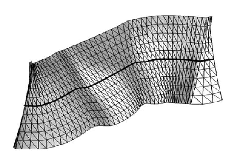
The extended surface of a landmark curve(the thick black line) is represented as a triangular mesh.
3.3 Adaptive Numerical Schemes
Before we present our adaptive numerical schemes, we first define the notion of connectedness between neighboring grid points for the purpose of incorporating landmark constraints. For two neighboring grid points x1 and x2, we call them connected if the line segment connecting x1 and x2 does not cross the extended surface of any landmark curve. In the derivation below, we will use integer indices such as (i, j, k) to denote points in the 3D Cartesian grid.
In designing numerical schemes to solve (10) and taking into account the boundary conditions, our basic strategy is to prevent the numerical stencil used in computing partial gradients of u from crossing the extended surface of any landmark curve. This blocks the diffusion from crossing such surfaces in the narrow band of ℳ. Since only up to second order gradients are used in solving (10), we demonstrate below the first and second order adaptive numerical schemes that take into account the boundary conditions carried on the extended surfaces of sulcal curves.
Let the three components of the map u be denoted as u = [u1 u2 u3]. The forward difference scheme of the first order gradient of up(p = 1, 2, 3) at the point (i, j, k) is defined as:
| (13) |
where h is the sampling interval of the grid, and is the interpolated value of up at the intersection of the line segment connecting (i, j, k) and (i + 1, j, k) and the extended surface of a landmark curve. The numerical stencil used here in computing includes two points (i, j, k) and (i + 1, j, k). If they are connected, the usual first order forward difference scheme is adopted; but if they are not, the flow between these two points should be blocked and we assume a constant extension of the boundary condition from the point of intersection to (i + 1, j, k). Thus the boundary value from the extended surfaces is used to replace to compute . Using the same method, the first order difference operators , , , , can also be defined.
To demonstrate second order numerical schemes, we define the operator in the x direction as follows:
| (14) |
where with as the interpolated value of up at the intersection between the line segment connecting (i, j, k) and (i − 1, j, k) and the extended surface of a landmark curve. The numerical stencil used for computing includes three points (i − 1, j, k), (i, j, k) and (i + 1, j, k). The case that (i, j, k) and (i + 1, j, k) could be disconnected is already handled in the definition of . If (i − 1, j, k) and (i, j, k) are connected, the usual first forward then backward scheme is used. If these two points are disconnected, we once again assume constant extension of the boundary condition from the extended surface and block the flow between them by using the interpolated to replace . Following the same principle, we can define and similarly.
We next assemble all the building blocks of our numerical schemes to solve the PDE in (10) with landmark constraints. At time t, we denote the map u at a point (i, j, k) as uijk(t), and we want to derive the update scheme to compute uijk (t + 1) at the next time step. If we ignore the projection operator to the target surface ∏ψ(uijk(t)) for a moment, we can treat each component of u separately because:
| (15) |
Let (p = 1, 2, 3). Following (Mémoli et al., 2004a), we approximate the gradient with the forward difference scheme and the divergence with a backward difference scheme. The numerical scheme for computing is:
where the projection matrix ∏∇ϕijk at point (i, j, k) is computed using the standard central difference scheme. Let . Our complete numerical scheme to solve (10) with landmark constraints is as follows:
| (16) |
where Δt is the time step, which is selected to be bounded by the stability condition in (Mémoli et al., 2004a). The projection operator ∏Δψ(uijk(t)) is also computed using the standard central difference scheme.
The update equation in (16) for the harmonic map is an explicit numerical scheme which we chose for its simplicity. For numerical efficiency, other schemes such as implicit schemes can also be used and are part of our future research. Our method of incorporating boundary conditions, however, is general and can be easily adapted into these more advanced numerical schemes.
4 Initialization Using Landmark Context
The numerical algorithm developed in the previous section modifies the gradient descent flow of the harmonic energy with adaptive operators for computing first and second order partial gradients, so it is still essentially a steepest descent algorithm. This makes the selection of a good initialization a critical step for a successful mapping since the optimization of the variational problem in (11) and (12) is non-convex as pointed out in section 2.
For a high dimensional optimization problem such as cortical mapping, it appears at first to be a daunting task to find a suitable initial map. However the search space can be greatly reduced if we utilize our prior knowledge about the map. First the value of the map u on the set of sulcal landmark curves on the source manifold ℳ is already given as our boundary condition. We also know that u should be interpolated smoothly in areas between these sulcal curves, which is the point of minimizing the harmonic energy. Based on this knowledge, we propose a novel front propagation type approach to find a good initial map. All the sulcal curves act as the source of the front propagation in the beginning of our algorithm. We then move outward to find the map at their neighboring points by searching locally for the best correlation of a feature we call landmark context, which is defined at each point on both the source and target cortical surface. These newly mapped points then serve as the current source of the front and we repeat the above process until the whole source cortical surface is covered.
Our definition of the landmark context feature on the cortical surface is partly motivated by the idea of shape context (Belongie et al., 2002) in computer vision. For a shape viewed as a point set, the shape context feature at each point is defined as a distribution of the relative locations of other points on the shape with respect to this point. This has proved to be a very powerful idea for shape matching and object recognition (Tu and Yuille, 2004). Following the same principle, we define the landmark context for each point as follows:
| (17) |
where is the set of sulcal landmark curves on ℳ and is the geodesic distance from to p. Compared with the feature of shape context, our landmark context feature is computationally more tractable. Its calculation only involves the computation of the distance transform for a limited set of curves, while shape context needs to compute at each point the distribution of the rest of the shape. If we view the landmark curves as the axes of a coordinate system on the cortex, the distances to them at each point intuitively play the role of coordinates and give us a very good indicator of the relative location of the point on the cortical surface.
In searching for the initial map with landmark context, we find it convenient to use the triangular mesh representation of the cortical surfaces, which is typically the original representation of our data, since we need to work directly with points on the surface and their relation to landmarks. Once we find the initial map on the triangular mesh, we then embed the mesh into the narrow band of the level-set function ϕ and extend the map along the normal direction to the whole narrow band. This is used as the initialization of the iterative PDE-based algorithm described in section 3.
Without causing confusion, we will still use the notation ℳ and to denote the triangular mesh representation of the source and target cortical surface. Each of them is composed of a set of vertices and faces. The set of sulcal curves on ℳ is
, with the corresponding set of sulcal curves on as
. At the start of our algorithm, we compute the geodesic distance transform for each of the sulcal curve on ℳ and using the fast marching algorithm on triangular meshes ( Kimmel and Sethian, 1998). At each vertex of the meshes, we record its distance to all sulcal curves and form its landmark context. After this step, the landmark context is defined at each vertex of ℳ and .
We next find the initial map at vertices close to the landmark curves and use them as the starting point of the front propagation process over the triangular mesh ℳ. For a curve
on ℳ and its corresponding curve
on , we sample both of them uniformly into L points. For each of the L points on
, we find the closest vertex on ℳ and push it into a heap Hℳ. Similarly, for each of the L points of
, we find the closest vertex on and push it into a heap
. After this process is repeated for every pair of sulcal landmark curves on ℳ and , we have two heaps Hℳ and
with matched vertices and are ready to march outward. Note that the same vertex can appear multiple times in a heap since more than one point on a sulcal curve can have the same vertex as its closest match. For the heap Hℳ, this means one vertex is matched to multiple vertices in . Our algorithm simply uses the first match in
as the initial map. For the heap
, this means one vertex in is matched by multiple vertices in ℳ, and we just leave it as it is and let the PDE-based approach improve the map.
Once both heaps are initialized, we start the front propagation process to find the initial map for all vertices on ℳ. The matched vertices in Hℳ and
are used as seed points for finding new matched pairs. In each step we pop out the first element of Hℳ and
, and denote them as pS and pT respectively. If the match result at the point pS has already been found, we skip further processing and move on to the next pair of matched vertices in the heaps. Otherwise, we save pT as the mapping result of pS and search the mapping for neighboring vertices of pS. To clarify the meaning of neighbors in a mesh, we use the notion of the k-ring neighborhood of a vertex that is defined as the set of vertices within k edges away from this vertex. For each vertex in the 1-ring neighborhood of pS that has not found a match in , we search for its match locally in a P-ring neighborhood of pT with the highest correlation of their landmark context, which means they have the most similar relative location with respect to the set of sulcal curves on the corresponding cortex. Typically we choose P = 5 in our experiments. Once we find a match, we push them into Hℳ and
. After the search is finished for all 1-ring neighbors of pS, we pop out new elements from Hℳ and
and continue the above procedure until the heaps become empty.
As a summary, the complete algorithm of finding the initial map is listed in Table I.
Table 1.
The algorithm for finding the initial map using landmark context
|
5 Extension To Energy With Data Terms
We have so far developed a complete solution for direct cortical mapping by minimizing the harmonic energy with landmark constraints. But the implicit mapping technique offers us lots of flexibility in defining and minimizing energy functions on surfaces. In this section, we demonstrate this generality by extending the energy function in (11) with data terms.
We first define two feature functions and on the source and target cortical surface. We limit the feature to be scalar for simplicity, but the extension to vectorial features is straightforward. We also define a weight function as follows:
| (18) |
for each
. Here
is the minimum of the landmark context at p and h is the sampling interval of the grid. The weight function w decreases from one to 2/(1 + e10) as d(p) approaches zero. Using the fast marching algorithm, we extend f1, f2 and w to the narrow band of ϕ and ψ along the normal direction, which are the implicit representations of ℳ and . We then define our new energy function that combines the harmonic energy with a data term:

where λ is a non-negative regularization parameter. The data term in the new energy function is a weighted least square term that penalizes the difference between the feature function on the source and cortical surface. Since the weight function is almost zero in the neighborhood of sulcal curves, the data term will not violate the landmark constraints in (12).
After computing the first variation of the energy, we obtain the gradient descent flow of the map u as:
| (20) |
where the term Π∇ψ(u(x,t)) ∇f2(u) is the intrinsic gradient of f2 at . To solve this equation numerically and minimize the new energy function, we apply the adaptive schemes we developed in section 3 and obtain the following numerical scheme that updates uijk from time t to t + 1:
| (21) |
where δuijk(t) and Π∇ψ(uijk(t)) are the same as in (16), and the standard central difference scheme is used to compute ∇ f2(uijk(t)).
Besides the least square energy in (19), we can also incorporate other data terms into our extended energy function. For example, it can be the correlation between features, or their mutual information (Wells et al., 1996; Wang et al., 2005a). Thus our method opens up an important opportunity for designing customized data terms that suit the need of specific brain mapping problems.
6 Experimental Results
The inputs to our direct mapping method include both the cortical surfaces and the sulcal landmark curves defined on the two surfaces. The cortical surfaces used in our experiments are generated using the algorithm in (MacDonald, 1998) in the form of triangular meshes, which were used in many neuroscience studies (Thompson et al., 2004). While the cortical surface generated from this algorithm may not reach the deepest parts of some sulcal regions, it captures all the major sulci and thus could be viewed as an approximation at certain scale of the pial surface that represents the outer boundary of the cortex. It is also convenient for manual tracing of sulcal landmarks on these smooth surfaces. But the direct cortical mapping method presented here is not limited to specific surface models and can also be applied to cortical surfaces extracted from other algorithms.
We compute the implicit representations of the cortical surfaces by converting each of them to a signed distance function with the fast marching algorithm. For the solution of PDEs on implicit surfaces, the signed distance function is only defined in a narrow band. In our numerical algorithms, we use an effcient sparse data structure DTGrid proposed in (Nielsen and Museth, in press) to represent the narrow band. The set of landmark curves are delineated using a protocol that defines 36 sulcal and landmark curves. Each curve is sampled to a fixed number of points with curve length parameterization. One-to-one correspondences between curves on different cortexes can then be established and used as constraints in our variational framework.
In our first two experiments, we compute the direct map between a pair of cortices by minimizing the harmonic energy in (8) and the extended energy in (19). These two experiments illustrate various properties of our direct mapping method. After that, we apply our algorithm to a group of 30 subjects and compare the property of metric distortion with a parametric mapping method. Finally, we apply our method to the application of cortical atlas construction and variability analysis.
6.1 Direct Mapping of Two Cortices with Harmonic Energy
In this experiment, we compute a map from a source cortex to a target cortex by minimizing the harmonic energy with sulcal landmark constraints. This experiment will illustrate the role of each step in our algorithm towards the generation of a direct map. The results from this experiment will also demonstrate the convergence property of our algorithm in optimizing the harmonic energy and its ability to improve the conformality of the mapping by reducing angle distortions.
The data used in this experiment, including the source and target cortex and their landmark curves, are shown in Fig. 4. A set of extend surfaces, as shown in Fig. 5, are constructed from the landmark curves in Fig. 4(c) using the algorithm proposed in section 3 to extend the boundary condition off the source cortical surface.
Fig. 4. The input data for the mapping of two cortical surfaces.
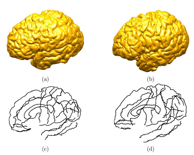
(a) The source cortex. (b) The target cortex. (c) The set of sulcal landmark curves of the source cortex. (d) The set of sulcal landmark curves of the target cortex.
Fig. 5.
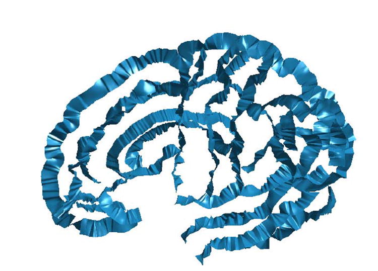
The set of extended surfaces constructed from all the landmark curves of the source cortical surface.
For the triangular mesh of both the source and target cortical surfaces, we then compute the landmark context at each vertex using the set of landmark curves. Based on this result, an initial map is then computed using the algorithm developed in section 4. To visualize this map, we first pull a checkerboard pattern onto the source cortex using the conformal mapping algorithm in (Gu et al., 2004). The lateral and medial view of this pattern on the source cortex are shown in Fig. 6(a) and (b). The checkerboard pattern is then projected onto the target cortex with the initial map and the results are shown in Fig. 6(c) and (d). Even though the initial map may appear quite good, we can clearly see noisy distortions at various locations such as the regions inside the black ellipses in both views. The initial map defined on the triangular mesh is extended to the narrow band along normal directions with the fast marching algorithm such that ∇u · ∇ϕ = 0.
Fig. 6. Visualization of the direct map between cortical surfaces in both the lateral and medial view.
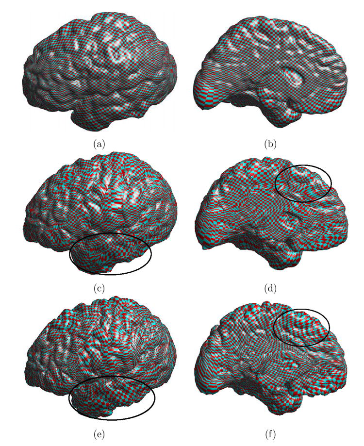
(a) and (b) are the checkerboard pattern on the source cortex. (c) and (d) are the checkerboard pattern mapped onto the target cortex using the initial map. (e) and (f) are the checkerboard pattern mapped onto the target cortex using the direct map computed from our algorithm. The smoothness of the map is improved as can be seen in regions inside the black ellipses.
With the initial map provided from the previous step, we start our numerical algorithm that solves the PDE in (10). The parameters in our algorithm are chosen as: the sampling interval of the grid h = 1 mm and the time step Δt = 0.1. To prevent the map u from drifting away from the target surface due to numerical errors, we project it back onto the target surface using the operator Πψ(uijk(t)) every 5 iterations. As a common practice in level-set techniques, the map is also re-initialized every 30 iterations such that the property ∇u·∇ϕ = 0 is approximately satisfied. The final mapping result is obtained after 5000 iterations. The total computation time is around 4 hours on a 3.19GHz PC.
In this iterative solution process, the harmonic energy function is reduced over time and converges toward the end of iterations as we show in Fig. 7. The direct map computed from our algorithm is visualized in Fig. 6(e) and (f) by projecting the checkerboard pattern on the source cortical surface shown in Fig. 6(a) and (b) to the target cortical surface. In comparison with the projected pattern using the initial map as shown in Fig. 6(c) and (d), we can see clearly that the smoothness of the map is improved significantly, for example in regions highlighted by the black ellipses. This is the desired result from the minimization of the harmonic energy. Because of our adaptive numerical schemes, the landmark constraints are maintained as we solve the PDE over time. To illustrate this point, we have plotted the final map on seven major sulcal curves in Fig. 8 and we can see clearly the landmark constraints are satisfied. This shows that a smooth map is obtained while satisfying the landmark constraints.
Fig. 7.
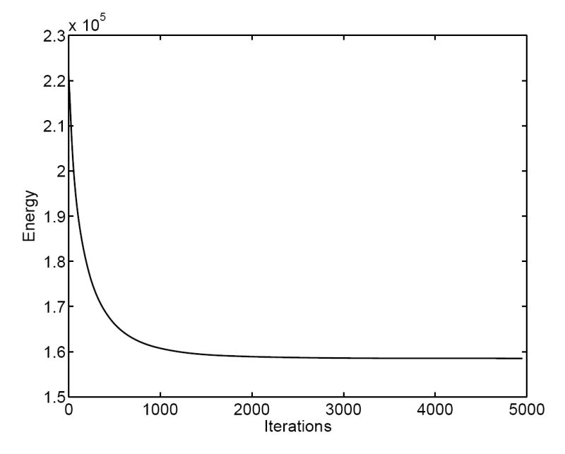
The energy decreases over the solution process.
Fig. 8.
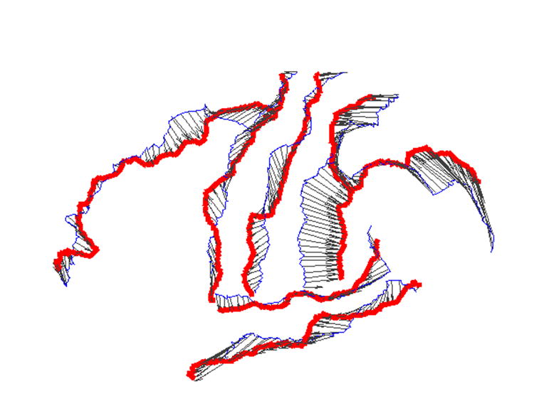
The direct map on seven major sulcal curves. The thin and blue lines are the sulcal curves on the source cortex and the thick and red lines are the sulcal curves on the target cortex. The map is visualized as the displacement vector fields on the sulcal curves of the source cortex.
An important property of the harmonic map is that it is also conformal when the target surface is of non-negative curvature (Gu et al., 2004). Even though there is no such guarantee in the direct map we computed because of the convoluted nature of the target surface and the presence of landmark constraints, we still observe in our experiment the improvement in conformality as the harmonic energy is minimized. To illustrate this property, we computed the angle distortions in the checkerboard pattern as we project it onto the target cortex. The histogram of the angle distortions resulted from the initial and final map are plotted in Fig. 9 (a) and (b). The mean of both histograms are approximately zero, but the standard deviation improves from 31.8831° to 26.5888°. This shows the magnitude of angle distortions are reduced as the harmonic energy is minimized.
Fig. 9. The effect of improving angle distortions with the direct map.
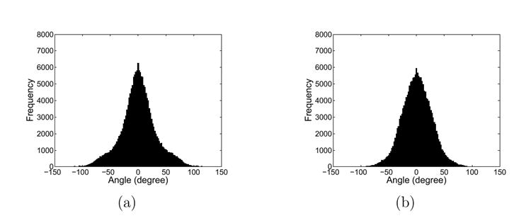
(a) The distribution of angle distortions from the initial map (mean = 0.5726°, std = 31.8831°. (b) The distribution of angle distortions from the direct map (mean = 0.9208°, std = 26.5888°).
The above experiment demonstrates that a smooth map between the source and target cortical surface is generated from our direct mapping algorithm. For validation purposes, we have also applied the above process to map the source cortical surface in Fig. 4(a) to itself. We then measure the distance between each vertex and its image under the resulting mapping to quantify numerical accuracy. Because of the finite resolution of the implicit representation, this distance will not be zero but should be on the same order as the grid resolution. Indeed the result verifies our intuition and the average distance over all vertices is 0.47mm, which is less than the grid interval that we chose as h = 1mm to match the resolution of the input triangular mesh representation of the cortical surfaces.
6.2 Cortical Mapping with Data Terms
In the second experiment, we demonstrate direct cortical mapping from the minimization of the energy in (19) with both the harmonic energy and a data term. We choose the feature f1 and f2 as the mean curvature of the cortical surfaces in this experiment. By penalizing the difference between mean curvature in the energy function, our goal is to obtain a smooth map that also matches similar geometric property.
We use the same data in the first experiment as shown in Fig. 4. The mean curvature of the source and target cortex are shown in Fig. 10. The regularization parameter is chosen as λ = 60. Because of the extra data term, we choose a smaller time step Δt = 0.01 for numerical stability. We use the result from the first experiment as our initial map and update it iteratively according to (21) to compute the minimizer of the energy in (19). The total energy converges over time as shown in Fig. 11(a) and we obtain the final result after 3000 iterations. As in the first experiment, we visualize the result by mapping the checkerboard pattern on the source cortex in Fig. 6 (a) and (b) to the target cortex in Fig. 12 (a) and (b).
Fig. 10. The mean curvature map on cortical surfaces.
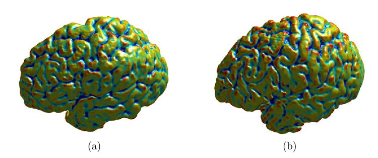
(a) The source cortex. (b) The target cortex.
Fig. 11. The change of the energy functions over time.
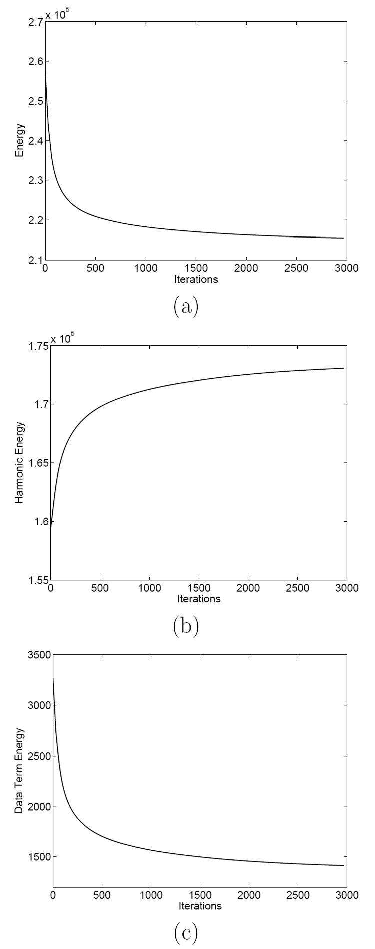
(a) The total energy with both the harmonic energy and the data term. (b) The harmonic energy. (c) The data term energy.
Fig. 12. Visualization of the map computed from the minimization of the energy with the least square data term.
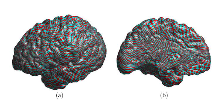
(a) The lateral view. (b) The medial view.
Comparing the projected checkerboard pattern in Fig. 12 (a) and (b) to that in Fig. 6 (e) and (f), we can see it is less smooth in various locations, such as the frontal lobe. This is reflected in the monotonic increase of the harmonic energy, shown in Fig. 11(b), as the total energy is minimized. It shows that the incorporation of the data term shifts the map from its initial value as the minimizer of the harmonic energy. We have also plotted in Fig. 11(c) the change of the data term energy, which is the weighted least square of the difference between the mean curvature on the two cortices. We can see it decreases over time and reduces to less than half of its initial value. This shows quantitatively we have a better match of the mean curvature profile between the source and target cortex.
6.3 Quantitative Comparisons with a Parametric Mapping Method
In this section, we compare the metric distortion property of our direct mapping method and a parametric mapping method. Since data terms are not included for most parametric mapping algorithms with landmark constraints, we use only the harmonic energy in our comparison. With sulcal landmark constraints, the goal of our direct mapping method is to compute a map that interpolates smoothly between these landmark curves. Ideally the map should be as close as possible to an isometry up to a scaling factor for regions between corresponding landmark curves on the source and target cortical surfaces. To validate this property, we will first propose an approach to measure the metric distortion of a map between cortices with landmark constraints. Quantitative comparisons are then performed between our direct mapping algorithm and a popular parametric mapping algorithm on a group of 30 subjects.
For ease of comparison with parametric approaches, we define the metric distortion
measure in terms of the triangular mesh representation of cortical surfaces. Let ℳ and denote two triangular meshes and u the mapping from ℳ to that establishes a one to one correspondence between vertices of ℳ and . For a vertex x in the source mesh ℳ, we can define a circular patch C(x) on ℳ as its geodesic neighborhood of radius r. Let the set of vertices that fall inside this patch C(x) be denoted as
and their geodesic distances to x as
. This set of geodesic distances can be organized into a lower triangular matrix T with its elements defined as
. Correspondingly, we have the set of vertices
inside the patch u(C(x)) on the target mesh . Their geodesic distances to u(x) are denoted as
and they can also be organized into a lower triangular matrix T* with its elements defined as
. Following (Tosun et al., 2004), we define as follows a metric distortion measure to test the quality of the map locally:
| (22) |
This measure quantifies the metric distortion from the source patch C(x) to the target patch u(C(x)). The lower the measure ℐ, the more similar are the two patches. This measure is zero when the map is locally an isometry up to a scaling factor from C(x) to u(C(x)), in which case is simply a scaling of .
Even though the measure ℐ in (22) is defined formally as in (Tosun et al., 2004), the scenario of its application here is different. In (Tosun et al., 2004), it is used to measure the global metric distortion over the whole cortex under spherical mapping with no landmark constraints. In a cortex to cortex mapping, however, each part of the cortex is stretched or compressed differently due to enforcement of the landmark constraints. To quantify how smooth the boundary conditions are interpolated between sulcal curves, we should avoid mixing different interpolation effects across different sides of these curves. Thus the patches used for the evaluation of metric distortions should not cross any sulcal curves. For a given radius r, this can be ensured by choosing the center point of the patch as those vertices x with min , where is the landmark context of x computed from the set of landmark curves on ℳ.
Using the metric distortion measure ℐ, we next compare our algorithm experimentally with a popular parametric approach proposed in (Thompson et al., 2000b, 2004). For a source cortex and a target cortex, this approach first maps them to spherical coordinates and then solves a system of partial differential equations governed by the Cauchy-Navier differential operator to compute the map. The covariant forms of the differential operators are used to take into account the Riemannian metric of the cortical surfaces. Once the map is computed in the spherical domain, it can be pulled back to the original cortices and we denote it as , where ℳ and are triangular mesh representations of the source and target cortex. With our direct mapping approach, we also compute a map u2 for the same pair of cortices without the intermediate parameterization steps. Since the map u2 is defined in a narrow band of the source cortex, we can obtain its value on each vertex of ℳ easily using simple linear interpolations on the Cartesian grid. The image of ℳ on the target cortex under the map u2 is denoted as .
In our experiment, we compare the metric distortion properties of the two different mapping methods on a group of 30 cortices. We divide this group into 15 pairs randomly such that each pair has a source cortex and a target cortex. For each pair, we compute both the map with the parametric approach and the map with our direct mapping method. For both u1 and u2, the metric distortion measure ℐ is computed at 5000 randomly selected circular patches of radius r = 5 on the source cortex ℳ. As we pointed out above, these patches do not cross any sulcal curves. The mean and standard deviation of the metric distortion measure at these 5000 patches are computed for both u1 and u2 and plotted for the whole group in Fig. 13(a) and (b). From these plots, we can see that our direct mapping algorithm performs better in terms of both the mean and standard deviation of the metric distortion.
Fig. 13. A comparison of the metric distortion property of the direct and parametric mapping algorithm.
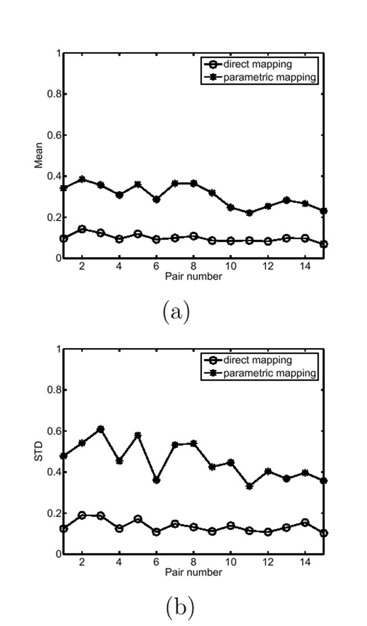
(a) The mean of the metric distortions on each pair. (b) The standard deviation of the metric distortions on each pair.
The above experiment shows that metric is better preserved in the direct map computed from the minimization of the harmonic energy, but we readily acknowledge that this is far from a thorough comparison between our direct mapping method and parametric mapping approaches, which is a very difficult task because both types of methods have their relative strength and weakness. The biggest advantage of our direct mapping method is that the whole mapping process is simplified by skipping the intermediate parameterization steps. The direct mapping method is also flexible in that it can incorporate variational energies with generic data terms. The parametric mapping approach, however, does have advantages in ensuring the diffeomorphic property of the map. The Eells-Sampson theorem (Eells and Sampson, 1964) tells us that the harmonic map from the cortical surface to the sphere is a diffeomorphism. The 2D warping process that matches landmark curves can also be guaranteed diffeomorphic with the work of computing large deformation diffeomorphisms (Christensen et al., 1996; Joshi and Miller, 2000). This ensures the final cortex to cortex map to be a diffeomorphism. Currently our direct mapping method is not provably diffeomorphic, but our experimental results demonstrate that it can obtain smooth maps of good metric preserving quality. Theoretically it is also possible for the heat flow of harmonic maps to have singularities under boundary constraints (Hardt, 1997). Finite-time blow-ups of a heat flow that maps from a disk to the sphere were reported in (Chang et al., 1992). But practically the direct cortical mapping method is very stable in our experience, probably due to the constraints imposed by the sulcal landmarks. We illustrate next that this new method can be easily applied to typical brain mapping applications such as cortical atlas construction and variability analysis.
6.4 Application: Cortical Atlas Construction
Atlas construction is a critical step in brain mapping. It integrates information from multiple brains and offers a framework for visualization and many analysis tasks, such as brain variability and asymmetry (Toga et al., 2001). In this section, we demonstrate atlas construction from the results of our direct mapping method using conventional cortical atlas construction techniques based on parametric surface representations.
Let be a group of cortical surfaces represented as triangular meshes. Their implicit representations are correspondingly a group of signed distance functions . For simplicity we use ℳ0 as the source cortex and apply our direct mapping algorithm to compute maps from ϕ0 to with landmark constraints. The direct maps from our algorithm are computed in the narrow band of ℳ0 where its implicit representation ϕ0 is defined. To obtain values of the direct map on the vertices of ℳ0, we use linear interpolation. This provides us explicit maps on the triangular mesh ℳ0, which projects each vertex of ℳ0 onto . We also denote u0 as the identity map from ℳ0 onto itself. With these maps, we can construct the cortical atlas as the average of this group of cortical surfaces. The averaging process is defined formally as follows:
| (23) |
which defines that each vertex of the atlas is the mean of corresponding points on the set of cortical surfaces .
As a simple application of this atlas, we can compute the variability at each vertex of the cortical atlas and it is defined formally as:
| (24) |
where ∥ · ∥ denotes the l2 norm of vectors in . At each vertex of , this equation computes the variance of the coordinates of its corresponding points on established by the maps .
We present next experimental results of atlas construction from a group of nine left hemispheres as shown in Fig. 14. The cortex in the middle is used as the source cortex ℳ0 and we compute the map from this source cortex to the rest of eight cortices by minimizing the harmonic energy. After that, the cortical atlas is computed using (23) and shown from both the lateral and medial view in Fig. 15(a) and (b). Since sulcal landmark constraints are strictly followed in our direct mapping algorithm, major sulcal curves are still clearly visible in the atlas. Using the cortical atlas, we also computed the variability map using (24). The lateral and medial view of this map are shown in Fig. 16(a) and (b). From this map on the cortical atlas, we can observe that the frontal, temporal and parietal-occipital lobes exhibit different degrees of variability among this group of subjects.
Fig. 14.
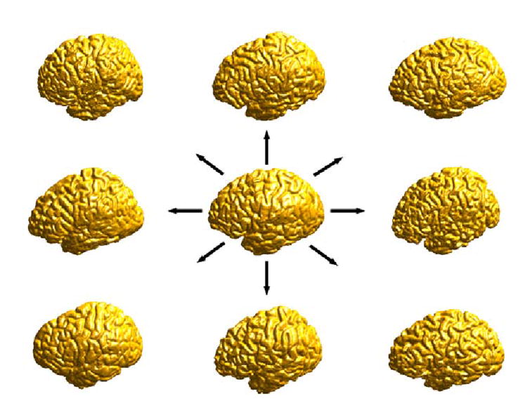
The construction of a cortical atlas from a group of nine subjects.
Fig. 15. The cortical atlas.
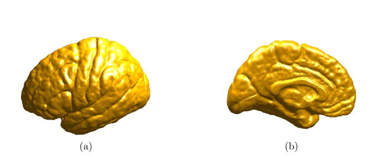
(a) Lateral view. (b) Medial view.
Fig. 16. The map of variability on the cortical atlas.
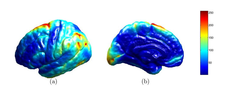
(a) Lateral view. (b) Medial View.
7 Conclusions
In this paper we proposed a direct mapping approach to compute maps between cortical surfaces with sulcal landmark constraints. This new method can avoid intermediate parameterizations in conventional approaches and greatly simplify the cortical mapping process. The direct mapping method is also very flexible and it can compute maps as the minimizer of variational energies with both the harmonic energy and general data fidelity terms. Experimental results demonstrate that our method can compute smooth maps between cortical surfaces while respecting landmark constraints. The application of our algorithm for cortical atlas construction and variability analysis in brain mapping were also presented.
Acknowledgments
This work was funded by the National Institutes of Health through the NIH Roadmap for Medical Research, Grant U54 RR021813 entitled Center for Computational Biology (CCB). Information on the National Centers for Biomedical Computing can be obtained from http://nihroadmap.nih.gov/bioinformatics.
Footnotes
Publisher's Disclaimer: This is a PDF file of an unedited manuscript that has been accepted for publication. As a service to our customers we are providing this early version of the manuscript. The manuscript will undergo copyediting, typesetting, and review of the resulting proof before it is published in its final citable form. Please note that during the production process errors may be discovered which could affect the content, and all legal disclaimers that apply to the journal pertain.
References
- 1.Angenent S, Haker S, Tannenbaum A, Kikinis R. On the Laplace-Beltrami operator and brain surface flattening. IEEE Trans Med Imag. 1999;18(8):700–711. doi: 10.1109/42.796283. [DOI] [PubMed] [Google Scholar]
- 2.Avants B, Gee JC. Geodesic estimation for large deformation anatomical shape averaging and interpolation. NeuroImage. 2004;23:S139–S150. doi: 10.1016/j.neuroimage.2004.07.010. [DOI] [PubMed] [Google Scholar]
- 3.Belongie S, Malik J, Puzicha J. Shape matching and object recognition using shape contexts. IEEE Trans Pattern Anal Machine Intell. 2002;24(4):509–522. [Google Scholar]
- 4.Bertalmío M, Cheng L, Osher S, Sapiro G. Variational problems and partial differential equations on implicit surfaces. Journal of Computational Physics. 2001;174(2):759–780. [Google Scholar]
- 5.Bertalmío M, Sapiro G, Randall R. Region tracking on level-sets methods. IEEE Trans Med Imag. 1999;18(5):448–451. doi: 10.1109/42.774172. [DOI] [PubMed] [Google Scholar]
- 6.Besl PJ, McKay N. A method for registration of 3-D shapes. IEEE Trans Pattern Anal Machine Intell. 1992;14(2):239–256. [Google Scholar]
- 7.Burchard P, Cheng LT, Merriman B, Osher S. Motion of curves constrained in three dimensions using a level set approach. Journal of Computational Physics. 2001;170(2):720–741. [Google Scholar]
- 8.Burger M. Finite element approximation of elliptic partial differential equations on implicit surfaces. UCLA CAM; Aug, 2005. pp. 05–46. Tech. Rep. [Google Scholar]
- 9.Cachier P, Mangin JF, Pennec X, Rivière D, Orfanos DP, Régis J, Ayache N. Multisubject non-rigid registration of brain MRI using intensity and geometric features. Proc MICCAI. 2001:734–742. [Google Scholar]
- 10.Carman GJ, Drury HA, Van Essen DC. Computational methods for reconstructing and unfolding the cerebral cortex. Ceberal cortex. 1995;5:506–517. doi: 10.1093/cercor/5.6.506. [DOI] [PubMed] [Google Scholar]
- 11.Chang KC, Ding WY, Ye R. Finite-time blow-up of the heat flow of harmonic maps from surfaces. J Differential Geom. 1992;36(2):507–515. [Google Scholar]
- 12.Chen S, Merriman B, Osher S, Smereka P. A simple level set method for solving Stefan problems. Journal of Computational Physics. 1997;135:8–29. [Google Scholar]
- 13.Cheng LT, Burchard P, Merriman B, Osher S. Motion of curves constrained on surfaces using a level-set approach. Journal of Computational Physics. 2002;175(2):604–644. [Google Scholar]
- 14.Christensen GE, Rabbitt RD, Miller MI. Deformable templates using large deformation kinematics. IEEE Trans Imag Process. 1996;5(10):1435–1447. doi: 10.1109/83.536892. [DOI] [PubMed] [Google Scholar]
- 15.Clouchoux C, Coulon O, Rivière D, Cachia A, Mangin JF, Régis J. Anatomically constrained surface parameterization for cortical localization. Proc MICCAI. 2005:344–351. doi: 10.1007/11566489_43. [DOI] [PubMed] [Google Scholar]
- 16.Collins DL, Goualher GL, Evans AC. Non-linear ceberal registration with sulcal constraints. Proc MICCAI. 1998:974–984. [Google Scholar]
- 17.Davatzikos C, Vaillant M, Letovsky S, Bryan RN, Prince JL, Resnick SM. A computerized approach for morphological analysis of the corpus callosum. Journal of Computer Assisted Tomography. 1996;20(1):88–97. doi: 10.1097/00004728-199601000-00017. [DOI] [PubMed] [Google Scholar]
- 18.Drury HA, Van Essen DC, Anderson CH, Lee CW, Coogan TA, Lewis JW. Computerized mappings of the cerebral cortex: A multiresolution flattening method and a surface-based coordinate system. J Cogn Neuro. 1996;8(1):1–28. doi: 10.1162/jocn.1996.8.1.1. [DOI] [PubMed] [Google Scholar]
- 19.Dupuis P, Grenander U, Miller MI. Variational problems on flows of diffeomorphisms for image matching. Quarterly of Applied Mathematics. 1998;LVI(3):587–600. [Google Scholar]
- 20.Eells J, Lemaire L. Two reports on harmonic maps. World Scientific; 1995. [Google Scholar]
- 21.Eells J, Sampson JH. Harmonic mappings of Riemannian manifolds. Ann J Math. 1964;86:109–160. [Google Scholar]
- 22.Fischl B, Sereno MI, Dale AM. Cortical surface-based analysis ii: Inflation, flattening, and a surface-based coordinate system. NeuroImage. 1999a;9(2):195–207. doi: 10.1006/nimg.1998.0396. [DOI] [PubMed] [Google Scholar]
- 23.Fischl B, Sereno MI, Tootell RBH, Dale AM. High-resolution intersubject averaging and a coordinate system for the cortical surface. Human Brain Mapping. 1999b;8:272–284. doi: 10.1002/(SICI)1097-0193(1999)8:4<272::AID-HBM10>3.0.CO;2-4. [DOI] [PMC free article] [PubMed] [Google Scholar]
- 24.Glaunes J, Vaillant M, Miller MI. Landmark matching via large deformation diffeomorphisms on the sphere. J Math Imaging Vis. 2004;20:179–200. [Google Scholar]
- 25.Greer J. An improvement of a recent Eulerian method for solving PDEs on general geometries. UCLA CAM; Jun, 2005. pp. 05–41. Tech. Rep. [Google Scholar]
- 26.Greer J, Bertozzi A, Sapiro G. Fourth order partial differential equations on general geometries. UCLA CAM; Mar, 2005. pp. 05–17. Tech. Rep. [Google Scholar]
- 27.Grenander U, Miller MI. Computational anatomy: An emerging discipline. Quarterly of Applied Mathematics. 1998;LVI(4):617–694. [Google Scholar]
- 28.Grossman R, Kiryati N, Kimmel R. Computational surface flattening: a voxel-based approach. IEEE Transactions on Pattern Analysis and Machine Intelligence. 2002;24(4):433–441. [Google Scholar]
- 29.Gu X, Wang Y, Chan TF, Thompson PM, Yau ST. Genus zero surface conformal mapping and its application to brain surface mapping. IEEE Trans Med Imag. 2004;23(8):949–958. doi: 10.1109/TMI.2004.831226. [DOI] [PubMed] [Google Scholar]
- 30.Hardt RM. Singularites of harmonic maps. Bulletin of the Americal Mathematical Society. 1997;34(1):15–34. [Google Scholar]
- 31.Hellier P, Barillot C. Coupling dense and landmark-based approaches for nonrigid registration. IEEE Trans Med Imag. 2003;22(2):217–227. doi: 10.1109/TMI.2002.808365. [DOI] [PubMed] [Google Scholar]
- 32.Hurdal MK, Bowers PL, Stephenson K, Sumners DWL, Rehm K, Schaper K, Rottenberg DA. Quasi-conformally flat mapping the human cerebellum. Proc MICCAI. 1999:279–286. [Google Scholar]
- 33.Hurdal MK, Stephenson K. Cortical cartography using the discrete conformal approach of circle packings. NeuroImage. 2004;23:S119–S128. doi: 10.1016/j.neuroimage.2004.07.018. [DOI] [PubMed] [Google Scholar]
- 34.Joshi A, Shattuck DW, Thompson PM, Leahy RM. Cortical surface parameterization by p-harmonic energy minimization. Proc IEEE Int Symp Biomed Imag. 2004:428–431. doi: 10.1109/ISBI.2004.1398566. [DOI] [PMC free article] [PubMed] [Google Scholar]
- 35.Joshi S, Miller MI. Landmark matching via large deformation diffeomorphisms. IEEE Trans Imag Process. 2000;9(8):1357–1370. doi: 10.1109/83.855431. [DOI] [PubMed] [Google Scholar]
- 36.Ju L, Stern J, Rehm K, Schaper K, Hurdal M, Rottenberg D. Cortical surface flattening using least square coformal mapping with minimal metric distortion. Proc IEEE Int Symp Biomed Imag. 2004:77–80. [Google Scholar]
- 37.Kimmel R, Sethian JA. Computing geodesic paths on manifolds. Proc Natl Acad Sci USA. 1998;95(15):8431–8435. doi: 10.1073/pnas.95.15.8431. [DOI] [PMC free article] [PubMed] [Google Scholar]
- 38.Leow A, Yu CL, Lee SJ, Huang SC, Protas H, Nicolson R, Hayashi KM, Toga AW, Thompson PM. Brain structural mapping using a novel hybrid implicit/explicit framework based on the level-set method. NeuroImage. 2005;24:910–927. doi: 10.1016/j.neuroimage.2004.09.022. [DOI] [PubMed] [Google Scholar]
- 39.MacDonald D. Ph.D. thesis. McGill Univ; Canada: 1998. A method for identifying geometrically simple surfaces from threee dimensional images. [Google Scholar]
- 40.Mémoli F, Sapiro G, Osher S. Solving variational problems and partial differential equations mapping into general target manifolds. Journal of Computational Physics. 2004a;195(1):263–292. [Google Scholar]
- 41.Mémoli F, Sapiro G, Thompson PM. Implicit brain imaging. Neuroimage. 2004b;23(Suppl 1):S179–S188. doi: 10.1016/j.neuroimage.2004.07.072. [DOI] [PubMed] [Google Scholar]
- 42.Mémoli F, Sapiro G, Thompson PM. Brain and surface warping via minimizing Lipschitz extensions. University of Minesota; 2006. Tech. Rep. IMA Preprint #2092. [Google Scholar]
- 43.Nielsen MB, Museth K. Dynamic Tubular Grid: An effcient data structure and algorithms for high resolution level sets. Journal of Scientific Computing in press. [Google Scholar]
- 44.Osher S, Sethian J. Fronts propagation with curvature-dependent speed: algorithms based on Hamilton-Jacobi formulations. Journal of computational physics. 1988;79(1):12–49. [Google Scholar]
- 45.Ratz A, Voigt A. PDE’s on surfaces – a diffuse interface approach. UCLA CAM; Nov, 2005. pp. 05–62. Tech. Rep. [Google Scholar]
- 46.Schwartz EL, Merker B. Computer-aided neuroanatomy: differential geometry of cortical surfaces and an optimal flattening algorithm. IEEE Computer Graphics and Applications. 1986;6(3):36–44. [Google Scholar]
- 47.Schwartz EL, Shaw A, Wolfson E. A numerical solution to the generalized mapmaker’s problem: flattening nonconvex polyhedral surfaces. IEEE Trans Pattern Anal Machine Intell. 1989;11(9):1005–1008. [Google Scholar]
- 48.Sereno MI, Dale AM, Liu A, Tootell RBH. A surface-based coordinate system for a canonical cortex. NeuroImage. 1996;3:S252. [Google Scholar]
- 49.Sethian J. A fast marching level set method for monotonically advancing fronts. Proc Nat Acad Sci. 1996;93(4):1591–1595. doi: 10.1073/pnas.93.4.1591. [DOI] [PMC free article] [PubMed] [Google Scholar]
- 50.Thompson PM, Giedd JN, Woods RP, MacDonald D, Evans AC, Toga AW. Growth patterns in the developing brain detected by using continuum-mechanical tensor maps. Nature. 2000a;404(6774):190–193. doi: 10.1038/35004593. [DOI] [PubMed] [Google Scholar]
- 51.Thompson PM, Hayashi KM, Sowell ER, Gogtay N, Giedd JN, Rapoport JL, de Zubicaray GI, Janke AL, Rose SE, Semple J, Doddrell DM, Wang Y, van Erp TGM, Cannon TD, Toga AW. Mapping cortical change in alzheimers disease, brain development, and schizophrenia. NeuroImage. 2004;23:S2–S18. doi: 10.1016/j.neuroimage.2004.07.071. [DOI] [PubMed] [Google Scholar]
- 52.Thompson PM, Toga AW. A surface-based technique for warping three-dimensional images of the brain. IEEE Trans Med Imag. 1996;15(4):1–16. doi: 10.1109/42.511745. [DOI] [PubMed] [Google Scholar]
- 53.Thompson PM, Woods RP, Mega MS, Toga AW. Mathematical/computational challenges in creating population-based brain atlases. Hum Brain Mapp. 2000b;9(2):81–92. doi: 10.1002/(SICI)1097-0193(200002)9:2<81::AID-HBM3>3.0.CO;2-8. [DOI] [PMC free article] [PubMed] [Google Scholar]
- 54.Timsari B, Leahy R. Optimization method for creating semi-isometric flat maps of the cerebral cortex. Proc SPIE Conf Med Imag. 2000:698–708. [Google Scholar]
- 55.Toga AW. Brain Warping. Academic Press; New York: 1998. [Google Scholar]
- 56.Toga AW, Thompson PM. Mapping brain asymmetry. Nat Rev Neurosci. 2003a;4(1):37–48. doi: 10.1038/nrn1009. [DOI] [PubMed] [Google Scholar]
- 57.Toga AW, Thompson PM. Temporal dynamics of brain anatomy. Annu Rev Biomed Eng. 2003b;5:119–145. doi: 10.1146/annurev.bioeng.5.040202.121611. [DOI] [PubMed] [Google Scholar]
- 58.Toga AW, Thompson PM, Mega MS, Narr KL, Blanton RE. Probabilistic approaches for atlasing normal and disease-specific brain variability. Anat Embryol. 2001;204:267–282. doi: 10.1007/s004290100198. [DOI] [PubMed] [Google Scholar]
- 59.Tosun D, Prince JL. Cortical surface alignment using geometry driven multispectral optical flow. Proc IPMI. 2005:480–492. doi: 10.1007/11505730_40. [DOI] [PubMed] [Google Scholar]
- 60.Tosun D, Rettmann ME, Prince JL. Mapping techniques for aligning sulci across multiple brains. Medical Image Analysis. 2004;8(3):295–309. doi: 10.1016/j.media.2004.06.020. [DOI] [PMC free article] [PubMed] [Google Scholar]
- 61.Tsitsiklis JN. Effcient algorithms for globally optimal trajectories. IEEE Trans Automat Contr. 1995 Sep;40(9):1528–1538. [Google Scholar]
- 62.Tu Z, Yuille AL. Shape matching and recognition: Using generative models and informative features. Proc ECCV. 2004;3:195–209. [Google Scholar]
- 63.Van Essen DC. A population-average, landmark- and surface-based (PALS) atlas of human cerebral cortex. NeuroImage. 2005;28(3):635–62. doi: 10.1016/j.neuroimage.2005.06.058. [DOI] [PubMed] [Google Scholar]
- 64.Van Essen DC, Drury HA, Joshi S, Miller MI. Functional and structural mapping of human cerebral cortex: solutions are in the surfaces. Proc Natl Acad Sci USA. 1998;95:788–795. doi: 10.1073/pnas.95.3.788. [DOI] [PMC free article] [PubMed] [Google Scholar]
- 65.Wang Y, Chiang MC, Thompson PM. Automated surface matching using mutual information applied to riemann surface structures. Proc MICCAI. 2005a:666–674. doi: 10.1007/11566489_82. [DOI] [PubMed] [Google Scholar]
- 66.Wang Y, Lui LM, Chan TF, Thompson PM. Optimization of brain conformal mapping with landmarks. Proc MICCAI. 2005b;2:675–683. doi: 10.1007/11566489_83. [DOI] [PubMed] [Google Scholar]
- 67.Wang Y, Peterson BS, Staib LH. Shape-based 3D surface correspondence using geodesics and local geometry. Proc CVPR. 2000;2:644–651. [Google Scholar]
- 68.Welker WI. The significance of foliation and fissuration of cerebellar cortex. the cerebellar folium as a fundamental unit of sensorimotor integration. Arch Ital Biol. 1990;128:87–109. [PubMed] [Google Scholar]
- 69.Wells WM, Viola P, Atsumi H, Nakajima S, Kikinis R. Multimodal volume registration by maximization of mutual information. Medical Image Analysis. 1996;1:35–52. doi: 10.1016/s1361-8415(01)80004-9. [DOI] [PubMed] [Google Scholar]