Calcium Sparks in Intact Skeletal Muscle Fibers of the Frog

Abstract

Calcium sparks were studied in frog intact skeletal muscle fibers using a home-built confocal scanner whose point-spread function was estimated to be ∼0.21 μm in x and y and ∼0.51 μm in z. Observations were made at 17–20°C on fibers from Rana pipiens and Rana temporaria. Fibers were studied in two external solutions: normal Ringer's ([K⁺] = 2.5 mM; estimated membrane potential, −80 to −90 mV) and elevated [K⁺] Ringer's (most frequently, [K⁺] = 13 mM; estimated membrane potential, −60 to −65 mV). The frequency of sparks was 0.04–0.05 sarcomere⁻¹ s⁻¹ in normal Ringer's; the frequency increased approximately tenfold in 13 mM [K⁺] Ringer's. Spark properties in each solution were similar for the two species; they were also similar when scanned in the x and the y directions. From fits of standard functional forms to the temporal and spatial profiles of the sparks, the following mean values were estimated for the morphological parameters: rise time, ∼4 ms; peak amplitude, ∼1 ΔF/F (change in fluorescence divided by resting fluorescence); decay time constant, ∼5 ms; full duration at half maximum (FDHM), ∼6 ms; late offset, ∼0.01 ΔF/F; full width at half maximum (FWHM), ∼1.0 μm; mass (calculated as amplitude × 1.206 × FWHM³), 1.3–1.9 μm³. Although the rise time is similar to that measured previously in frog cut fibers (5–6 ms; 17–23°C), cut fiber sparks have a longer duration (FDHM, 9–15 ms), a wider extent (FWHM, 1.3–2.3 μm), and a strikingly larger mass (by 3–10-fold). Possible explanations for the increase in mass in cut fibers are a reduction in the Ca²+ buffering power of myoplasm in cut fibers and an increase in the flux of Ca²+ during release.

INTRODUCTION

Calcium sparks are transient localized increases in fluorescence in muscle cells that contain a Ca²⁺ indicator, such as fluo-3 (Minta et al. 1989), that is highly fluorescent only when in the Ca²⁺-bound form. These signals were detected first in rat cardiac myocytes (Cheng et al. 1993) and, subsequently, in frog skeletal muscle cells (Tsugorka et al. 1995; Klein et al. 1996). They reflect a local elevation of myoplasmic free [Ca²⁺] that results from the brief opening of one RYR or a small cluster of RYRs, the Ca²⁺ release channels of the SR. Because calcium sparks represent an elementary type of SR Ca²⁺ release that can be elicited by membrane depolarization, their study may help to elucidate the mechanism of excitation-contraction coupling.

Most studies of sparks in frog skeletal muscle have used the cut fiber preparation (Hille and Campbell 1976). This consists of a short segment of fiber transected at one or both ends and exposed to an artificial internal solution. Because mobile molecules such as small ions, ATP, phosphocreatine, peptides, soluble proteins, divalent ions, etc., begin to diffuse out of a fiber immediately after cutting, additions are usually made to the internal solution to keep the concentrations of some of these constituents near the normal range. For example, because the internal concentrations of Ca²⁺ and Mg²⁺ strongly affect RYR function, Ca²⁺ and Mg²⁺ are usually added to the internal solution with divalent cation buffers to help maintain resting free [Ca²⁺] and [Mg²⁺] at nominal physiological levels (usually ∼0.1 μM and 0.5–1.0 mM, respectively). In spite of such precautions, abnormalities in the structure and function of cut fibers have been noted. For example, frog cut fibers appear to be more hydrated than intact fibers (inferred from fiber swelling; Irving et al. 1987) and the spatially averaged Ca²⁺ transient triggered by an action potential progressively broadens during the course of an experiment (Maylie et al. 1987). In addition, different methods for fiber preparation appear to introduce variability in results, as studies from different laboratories sometimes reveal important differences. Examples include differences in the rate of onset of Ca²⁺ inactivation of Ca²⁺ release (final time constant, ∼32 ms at 6–10°C [Schneider and Simon 1988] vs. ∼2 ms at 14–15°C [Jong et al. 1995]) and differences in the properties of Ca²⁺ sparks themselves (see discussion). These and other results indicate the importance of studying calcium sparks in intact fibers, where the RYRs function in their native environment.

In this article, we describe the properties of several thousand voltage-activated calcium sparks. These were recorded in frog intact single fibers that were microinjected with fluo-3 and bathed in elevated [K⁺] Ringer's (typically, 13 mM [K⁺]; estimated membrane potential, −60 to −65 mV). A home-built confocal microscope, similar to that described by Parker et al. 1997, was used for optical recording. The results show that sparks in intact fibers are more confined in time and space than those in cut fibers (Lacampagne et al. 1996, Lacampagne et al. 1998, Lacampagne et al. 1999; Klein et al. 1999; Ríos et al. 1999; Gonzalez et al. 2000a,Gonzalez et al. 2000b; Shtifman et al. 2000). Although the average spark rise time is similar in the two preparations (∼4 ms in intact fibers, 17–20°C; 5–6 ms in cut fibers, 17–23°C), the full duration at half maximum (FDHM) is briefer in intact fibers (∼6 vs. 9–15 ms) and full width at half maximum (FWHM) is narrower (∼1.0 vs. 1.3–2.3 μm). A more pronounced difference is found for spark “mass” (which, for an in-focus spark, is expected to be proportional to the volume integral of the change in fluo-3 fluorescence; see materials and methods); mass is 3–10 fold larger in cut fibers than in intact fibers.

Another difference between voltage-activated sparks in intact and cut fibers is evident during the late phase of a spark. Gonzalez et al. 2000a reported a late signal, which they termed “the ember.” They proposed that the ember represents the maintained release of Ca²⁺ by a single voltage-gated RYR that, at an earlier time, provided the Ca²⁺ that triggered the opening of the other RYRs responsible for the spark. The fluorescence increase that we detect in intact fibers at the time of the ember is 0.02 ΔF/F (change in fluorescence divided by resting fluorescence), which is about fivefold smaller than that reported by Gonzalez et al. 2000a.

Some of the results have been reported in abstract form (Hollingworth et al. 2000b, Hollingworth et al. 2001; Baylor et al. 2000, Baylor et al. 2001).

MATERIALS AND METHODS

Microscope Configuration and Procedures for Image Acquisition

The experiments were performed in the Department of Physiology at the University of Pennsylvania. A home-built confocal line scanner, similar to that described by Parker et al. 1997, was used to record fluorescence images from muscle fibers that contained fluo-3 (penta-potassium form; Molecular Probes, Inc.). Our instrument (Fig. 1) is organized around a Zeiss inverted microscope equipped with a Zeiss epifluorescence insert and an Olympus high numerical aperture water immersion objective (Plan-Apo 60×; 1.20 NA; working distance ∼200 μm). These optical elements, plus a set of lenses and mirrors, permitted the 488-nm light from a 25-mW argon ion laser to be focused as a diffraction-limited spot on the fiber. The laser was run in “light control” mode, which maintained a nearly ripple-free output at close to maximum power. The spot was moved along the fiber axis (x displacement) by rotation of a galvanometer scan mirror (S), which was driven by an approximately saw-tooth input to the mirror controller (Parker et al. 1997). In the return path, the longer wavelength fluorescent light was separated by a 495-nm dichroic mirror (D) in combination with a 500-nm long-pass filter (F2).

Figure 1.

Schematic of the home-built x-t scanner. The output from a 25-mW argon ion laser was focused onto a muscle fiber mounted in the experimental chamber (C) on the stage of a Zeiss IM35 inverted microscope. The excitation path traversed: a TTL-controlled shutter (S1; Coherent-Ealing), a 488-nm narrow band interference filter (F1; Chroma Technology Corp.), neutral density filter(s) that attenuated the beam intensity (ND), a beam expanding lens (BE; Newport), a 100% reflecting mirror (R; Newport); a dichroic mirror centered at 495 nm (D; Chroma), a scan mirror (S; Cambridge Technology) mounted in an aluminum housing (dashed), a 10× wide-field eye piece that functioned as the scan lens (SL; Nikon), a second shutter (S2), a relay lens (RL; Newport), a Zeiss epifluorescence insert (EI), and (not shown) a second reflective mirror, the nosepiece of the Zeiss microscope, and a high numerical aperture water immersion objective (Plan-Apo 60×, 1.2 NA; Olympus). The emission path traversed the same elements in reverse order back to D; then a long-pass filter (F2; model HQ-500-LP; Chroma); a confocal pinhole (P; diam ∼1.5 mm), which passed the bright central portion of an Airy disk; a beam-spitting prism (BS), which split the light into two paths of approximately equal intensity; converging lenses (not shown). Light detection used photon-counting avalanche photodiodes (APD 1 and 2; EG&G).

Data acquisition was controlled by a master timer/AD/DA unit (model IDA 12500; Indec Systems). DA output from the IDA unit supplied a synchronized voltage waveform to drive the mirror controller. A sample line scan usually consisted of 256 data points collected at 125 kHz (line scan period, 2.048 ms). The usable portion of the scan consisted of 215 points, which were collected during the linear displacement of the spot along a 43.0-μm length of fiber (0.20 μm per pixel). The remaining 41 points were collected during the fly-back of the scan mirror and were ignored. A unit x-t image consisted of 256 such line scans acquired in 524 ms.

The program controlling data acquisition was custom written in C7.0 (Microsoft Corp.). It used library links to elementary AD/DA functions supplied by Indec Systems, which were written in both assembly language and C. Our acquisition program, when run on a 266-MHz Pentium II computer, could acquire and store to disk an essentially unlimited stream of line scans without loss of data. However, most fiber runs consisted of only three continuous unit images, which comprised a 43.0-μm by 1.571-s x-t image (for technical reasons, the first scan line was always discarded). In a few experiments (see results), x-t images were also recorded with a briefer line scan period, 1.024 ms instead of 2.048 ms. To achieve the faster scan speed, the mirror excursion was reduced by slightly more than twofold. In this situation, there were 192 usable data points at a pixel separation of 0.09 μm, yielding a useful scan length of 17.3 μm.

As in the system described by Parker et al. 1997, fluorescence intensity was measured with photon-counting avalanche photodiodes (models SPCM-AQ-121 and SPCM-AQR-12; EG&G Inc.). Diodes of this type, if used in their linear range (up to ∼2 photon counts per μs), have a quantum efficiency of 50–60% at the wavelengths of fluo-3′s fluorescence (500–600 nm). For the detection of low light levels, they supplied the largest signal-to-noise ratio of four types of detectors tested (Tan et al. 1999). At higher intensities, the count rate does not increase linearly with intensity and the signal-to-noise ratio decreases accordingly. To maintain a high signal-to-noise ratio at higher intensities, the fluorescent light was split between two detectors (Fig. 1), so that the fluorescence intensity measured by each detector remained near the linear range (Wier et al. 2000). In our experiments, the average (uncorrected) resting intensity was typically 1–6 counts per μs per diode. This corresponds to 1–8 counts per μs per diode after correction for nonlinearity; this correction used the calibration curves supplied by the manufacturer (which were specific for each diode). Each diode output was converted to a voltage signal by a custom-built counter-to-voltage converter (Current Designs), which was sampled by the AD converter of the IDA unit. The images from the individual detectors, if viewed separately, appeared to be identical. In some experiments, only one avalanche photodiode was used. The results from these experiments were very similar to those in which two detectors were used. For analysis, the digitized pixel intensity levels were converted back to units of counts per microsecond and corrected for nonlinearity. If two detectors were used, the images from the individual detectors were summed.

In early experiments, a time-dependent decline was observed in the mean intensity of successive line scans in an image. Most of this decline was traced to light-induced warm up of optical filters F1 and ND located after shutter S1 (Fig. 1). This decline was reduced substantially by the use of a second shutter S2, which was opened after S1. The small residual decline in intensity was corrected as described below. Upon completion of scanning, a rotation of the scan mirror moved the laser spot off the fiber to avoid fiber damage.

Slow x-y scans (see Fig. 2 A, described below) were performed with a motorized drive that moved the vertical position of relay lens RL. At the fiber, this movement produced a linear displacement of the line scan in the y direction, i.e., the direction perpendicular to the normal scan direction. To match the pixel displacement in y to that in x (0.20 μm per point), the rate of data acquisition (and the laser intensity) were reduced by about an order of magnitude.

Figure 2.

(A) A sample fluorescence x-y image (215 pixels × 391 pixels) from a fluo-3–injected fiber in normal Ringer's. The vertical and horizontal white lines indicate the directions used for x-t and y-t scanning (parallel and perpendicular to the fiber axis, respectively). The length of each line is 43.0 μm, the most commonly used scan length. [Note: the image perspective is slightly asymmetric in x and y.] The bright punctate regions of fluorescence, termed hot spots, are discussed in materials and methods. (B) A fluorescence x-t image (217 × 767 pixels) from another fiber in normal Ringer's; the pixel separation was 0.20 μm in x (vertical) and 2.048 ms in t (horizontal) The top half of the image reveals a narrow ‘streaker’ that bleached with time (time constant, 0.2 s). The resting F(x) profile (right) was obtained as the time average of the final 255 line scans. (C) Magnified ΔF/F image of the streaker portion of the first 76 lines. (D, asterisks) (ΔF/F)(x) profile averaged from the lines in C. The curve is a least-squares fit to the profile of a Gaussian function (); the fit gave an estimate of 0.27 μm for the FWHM of the streaker. Fiber references: z080300b, R. pipiens (A); z082499b, R. temporaria (B–D).

Microscope Point-spread Function

The point-spread function (PSF) of the microscope was estimated from a series of x-y images of fluorescent beads (diameter 0.1 μm; Polysciences Inc.). The pixel separation in x and y was 0.10 μm and the z distance between images was 0.25 μm (z being the direction along the light path). The beads were immobilized by suspension in an agarose gel (30% sucrose + 0.5% agarose) that had solidified on the upper surface of a coverslip. The nominal refractive index of the gel, 1.38 (Hollingworth et al. 2000a), matches that expected for frog intact muscle fibers (Huxley and Niedergerke 1958). Intensities were measured from beads located 6–26 μm above the coverslip, and the data were fitted with Gaussian profiles (see below) to estimate values of FWHM in x, y, and z. The values obtained were 0.21 ± 0.01 μm in x, 0.21 ± 0.01 μm in y, and 0.51 ± 0.02 μm in z (mean ± SEM; N = 91). These values are similar to those obtained by Parker et al. 1997 and Wier et al. 2000 for 0.1 μm fluorescent beads immobilized on a coverslip: 0.25–0.3 μm in x and y, and 0.4–0.52 μm in z (1.4 NA; 40–63× oil objectives).

Fiber Preparation and Measurement Procedures

Most of the early experiments of this study were performed on intact single fibers isolated from leg muscles (iliofibularis and semitendinosus) of Rana temporaria. Later experiments, with more complete results, were usually performed on single fibers from Rana pipiens. An isolated fiber was mounted on an optical bench apparatus, stretched to a sarcomere length of ∼3.6 μm, and pressure-injected with fluo-3 (Harkins et al. 1993). The fiber was accepted for study if, in response to a single stimulated action potential, the peak of the spatially averaged ΔF/F signal was all or none and had a peak value greater than nine (range, 9.5–24; N = 27).

Somewhat surprisingly, the values of the spatially averaged ΔF/F elicited by an action potential were larger in the present study than in our previous studies. For fibers from R. temporaria, the increase in mean ΔF/F was about twofold: 14.2 ± 0.8 (N = 12) in this study versus 6.8 ± 0.5 (N = 15) in Harkins et al. 1993 and 6.5 ± 1.0 (N = 4) in Hollingworth et al. 2000a. The fibers from R. pipiens had even larger values of ΔF/F, 18.6 ± 0.9 (N = 15). Because smaller values of resting myoplasmic [Ca²⁺] ([Ca²⁺]_R) will produce smaller values of resting F and correspondingly larger values of ΔF/F, the larger ΔF/F values detected in the present study indicate that [Ca²⁺]_R was smaller than in our earlier studies (on the assumption that ΔF changes little with [Ca²⁺]_R; see results).

A possible explanation for a larger [Ca²⁺]_R in the experiments of Harkins et al. 1993 and Hollingworth et al. 2000a is that some slight local damage may have occurred as a result of the fluo-3 injections. In the experiments of Harkins et al., the tips of the injection pipettes tended to clog, so that relatively long impalements, ∼15 min, were required for the injections. In the present study, there was less difficulty with clogging, and impalements were much briefer, usually <3 min. A possible explanation for the higher values of ΔF/F observed in the fibers of R. pipiens versus R. temporaria (18.6 vs. 14.2, respectively) is that the R. pipiens were in better overall condition than the R. temporaria. R. pipiens, which are readily available within the United States, were ordered more frequently and in smaller numbers than R. temporaria, which were obtained from Ireland. As a result, R. pipiens were kept in hibernation for a shorter period of time before use.

After injection, the fiber was transferred to a different chamber and sarcomere length was set to ∼3.0 μm (range, 2.70–3.66 μm). Two L-shaped glass rods attached to microdrives on the chamber walls pressed the fiber downward so that the bottom surface of the fiber region that contained the injection site was 0.1–0.2 mm above the chamber floor, within the working distance of the microscope objective. The center of the chamber floor consisted of an 18-mm square coverslip, which was held by Vaseline on a Perspex rim and changed daily. The thickness of the coverslip (155 μm) was selected to match the adjustable coverslip setting on the collar of the microscope objective. The chamber was mounted on the stage of the microscope and the solution bathing the fiber (see below) was cooled to 17–20°C.

To avoid overexposure of the fiber to laser light, x-t images were recorded at different locations in x, y, and z. Typically, a continuous set of three x-t images was acquired at one z location. Then, the microscope focus was changed manually by ∼5 μm and another triplet of images was recorded. Several such runs were performed at different z locations (0–30 μm above the bottom surface of the fiber), after which the y recording location was changed by a slight translation (5–30 μm) of the stage perpendicular to the fiber axis. After similar runs at two to four different y locations, the microscope stage was translated in the x direction (along the fiber axis) by 50–250 μm, and a new series of recordings was made. With these procedures, up to several hundred images could be acquired from different regions of a fiber in a period of 30–60 min.

Resting sparks were measured in normal Ringer's solution (in mM: 120 NaCl, 2.5 KCl, 1.8 CaCl₂, 5 PIPES, pH 7.1) and voltage-activated sparks were measured in solutions containing elevated [K⁺], most frequently 13 mM [K⁺] (referred to as 13 mM [K⁺] Ringer's), achieved by the addition of K₂SO₄ to Ringer's. Membrane potential was not measured but is expected to be approximately −80 to −90 mV in normal Ringer's and approximately −60 to −65 mV in 13 mM [K⁺] Ringer's (Hodgkin and Horowicz 1959). Fiber diameters were measured before and after introduction of elevated [K⁺] Ringer's and did not change.

In experiments with solution changes, image runs were usually taken immediately before and after the solution change at the same x location. This permitted an estimation of the effect of the solution change on the resting fluorescence of fluo-3.

Estimation of Indicator Concentration

In four experiments, the method of Harkins et al. 1993 was used to estimate the myoplasmic concentration of indicator from fiber diameter and fluo-3′s resting absorbance (which is relatively independent of Ca²⁺ complexation), which were measured at the injection site on the optical bench apparatus ∼10 min after injection. This concentration and the value of fluo-3′s resting fluorescence were used to estimate a calibration factor that related the concentration of fluo-3 to the resting fluorescence intensity per fiber cross-sectional area. The mean of the calibration factors from the four fibers was used to estimate the indicator concentration in the remaining fibers. For the 27 fibers of this study, the fluo-3 concentration estimated shortly after injection was 225 ± 17 μM (mean ± SEM). Indicator concentration was not measured during confocal recording, which was performed 20–80 min after injection and usually 50–300 μm along the fiber axis from the injection site. From calculations based on one-dimensional diffusion of fluo-3, the average indicator concentration during confocal recording was estimated to be ∼100 μM.

Spark Detection

Programs for spark detection and analysis were written in the IDL programming language (Research Systems Inc.). Each x-t fluorescence intensity image, F(x,t), was first corrected for a small, time-dependent decay in fluorescence that likely arose from residual warm up of components in the light path (see above). For this correction, a decaying exponential plus sloping baseline was fitted to F(t), the fluorescence averaged from all x locations at different t. At each t, F(x,t) was then multiplied by the ratio of the fitted value of F(0) and the fitted value of F(t). The resulting F(x,t) image was then converted to a ΔF/F image: (ΔF/F)(x,t) = (F(x,t) − F(x))/F(x). F(x), the spatial profile of resting fluorescence, was initially estimated as the time average of all F(x,t).

Each image was processed by an automatic spark detection algorithm, which is similar to that described by Cheng et al. 1999. A 3 × 3 smoothed version of the ΔF/F image was scanned for possible sparks. A spark was identified if at least three consecutive pixels on a given scan line, and one contiguous pixel on the subsequent scan line had values of ΔF/F above a threshold value. F(x) was then recalculated from F(x,t) after exclusion of the regions identified as sparks, and a new ΔF/F image was calculated and the detection algorithm was repeated. This process was continued until the number of detected sparks and the points associated with these sparks remained unchanged. Threshold was set at ΔF/F = 0.3. Depending on resting fluorescence, this value was three to seven times the standard deviation of F(x,t) in the spark-excluded, 3 × 3 smoothed image. To find out whether spurious sparks might arise from noise, detection was also performed for negative ΔF/F with a threshold of −0.3. In 604 images in which 2,617 positive sparks were identified with the positive threshold, only one negative spark, in the noisiest image, was detected with the negative threshold. Because tests with smaller threshold values showed more spurious “negative” sparks, 0.3 appeared to be the minimum threshold at which all images could be reliably analyzed.

Spark Morphology

Spark profiles in time (t) and space (x) were calculated from the unsmoothed ΔF/F images, and spark morphological parameters were obtained from least-squares fits of functional forms to these profiles. The time profile was obtained from an average of three time lines located at the center of the spark in x. These data were least-squares fitted by , which is similar to the functional form used by Lacampagne et al. 1999:

1

Although there is no a priori reason to expect to exactly fit the time course of a spark, it can be used to characterize its main features. The data were usually fitted for 25 pixels preceding and 50 pixels after the spark peak (51.2 and 102.4 ms, respectively). assumes that ΔF/F has an initial value of A₀; at t₁, it increases abruptly with a time constant τ_on to a peak value at t₂. After peak, the spark is assumed to decay exponentially, with a time constant τ_off, to a final value of (A₀ + A₂). The 0–100% rise time (= t₂ − t₁), peak amplitude (= A₁(1 − exp(−(t₂ − t₁)/τ_on))), decay time constant (= τ_off), FDHM, and late offset (A₂) were obtained from the fitted curve. Because the rise time of most sparks occurred during one to three time points (2–6 ms), the value of τ_on could not be estimated accurately. Consequently, its value was fixed at 4 ms for all fits (see Shtifman et al., 2000 [p. 826]). This choice is not critical because the estimates of the fitted spark parameters were little changed with τ_on set to 2, 4, or 8 ms. As described in results, the mean values of rise time from measurements made with 2-ms line scans may be overestimated by 10–20%.

The spatial profile of a spark was obtained from an average of the two line scans recorded just before and just after t₂. A Gaussian function, , was fitted to the spatial profile by adjustment of parameters A₃, A_4, x₀, and var:

2

As was the case with , is not expected to exactly fit the data; it is used to approximately characterize the spatial spread of a spark. These data were usually fitted for 25 pixels (5.0 μm) on either side of the central location of the spark, x₀. The FWHM of the spark at time of peak was estimated with from the variance parameter, var:

3

About 15% of detected sparks could not be analyzed either because they were located near the edge of an image or because there was significant overlap with another spark in time or space. In addition, broad limits were applied to exclude atypical fluorescence events: 0.4 < rise time < 25 ms; 0 < τ_off < 20 ms; 2.5 ms ≤ FDHM ≤ 40 ms; offsets (A₁, A₂, A₃) between −0.15 and 0.15 ΔF/F; 0.3 < FWHM < 4 μm. About 6% of analyzed sparks failed to satisfy these limits.

Izu et al. 2001 noted that spark amplitudes recorded with their home-built confocal microscope were larger than spark amplitudes recorded with a commercial BioRad 600 microscope. Because their home-built microscope detected light intensity with avalanche photodiodes whereas the BioRad used photomultipliers, one possibility for the amplitude difference is that the avalanche detectors introduce error due to the nonlinear correction for intensity (see above). Any such error is not likely to be significant in our spark measurements. First, 68% of analyzed sparks had a corrected intensity level that, at peak, was ≤8 counts per μs per detector; thus, most spark measurements were made near the linear range of the detectors. Second, an analysis of the population of “in-focus” sparks (defined as the largest 5% of sparks collected from each experiment, total number = 158 sparks) revealed no dependence of spark amplitude on resting fluorescence intensity per detector. The values of resting intensity ranged between 0.5 and 7 counts/μs, and the best-fitted regression line of amplitude vs. resting intensity had a slope of 0.0320 ΔF/F per (counts per microsecond), which was not significantly different from zero (at P < 0.05).

Spark Mass

Following the concept of signal mass introduced by Sun et al. 1998 in their study of elementary calcium release events in oocytes, we define spark mass as the volume integral of ΔF/F:

4

In confocal experiments with fluo-3, (ΔF/F)(x,y,z) is given by the convolution of the microscope PSF with Δ[Ffluo]/[Ffluo]_R; the subscript R denotes the resting state. The concentration variable [Ffluo] () is introduced because Ca²⁺-free fluo-3 is weakly fluorescent. It is equal to the value of [Ca-fluo-3] that would give the same fluorescence as a mixture of [Ca-fluo-3] and [fluo-3]:

5

[Ca-fluo-3] and [fluo-3] are the concentrations of Ca²⁺-bound and Ca²⁺-free fluo-3, respectively, and F_min and F_max represent the fluorescence intensity of Ca²⁺-free and Ca²⁺-bound fluo-3, respectively. In myoplasm, F_min/F_max ≈ 0.01 (Harkins et al. 1993). Because mass is equal to the volume integral of Δ[Ffluo]/[Ffluo]_R (unpublished theoretical analysis). the product of mass and [Ffluo]_R gives the total increase in Ffluo (in moles). This increase closely approximates the total increase in Ca-fluo-3 (in moles).

Because measurements of ΔF/F are usually limited to scans in x at one location in the y-z plane, some approximations are required to calculate spark mass from these measurements. First, we assume that the scan line runs through the location of Ca²⁺ release (“in-focus spark”), which will be taken as the origin of the coordinate system, (0,0,0). Second, we assume that (ΔF/F)(x,y,z) can be approximated as the product of three Gaussians (compare with ):

6

in which A is the signal amplitude at the origin. gives:

7

Third, we assume that the gaussians are isotropic in space (var_x = var_y = var_z). The last two assumptions may introduce some error because the spatial spread of Ffluo may not be Gaussian and isotropic, and the microscope PSF is not isotropic (var_z > var_y = var_x). Substitution of in (with var = var_x = var_y = var_z) gives:

8

is used in results to estimate spark mass from the fitted values of amplitude and FWHM (see previous section). Spark mass is considered in this article primarily to emphasize the 3-D nature of a spark and to permit additional comparisons with sparks measured in other preparations. Spark mass will be explored more fully in a forthcoming article. Preliminary calculations for this article indicate that underestimates, by about one third, the mass of an in-focus simulated spark that is calculated with .

A somewhat different method was used by Shirokova et al. 1999 to estimate spark mass. They assumed that the volume of spark mass can be approximated from the sphere that intersects the spark at half amplitude. This gives :

9

which yields a value of mass that is 0.434 times that calculated with .

An Upper Limit for Microscope FWHM_X in Muscle Fibers

Most images recorded in this study were x-t scans. Toward the end of some experiments, however, occasional x-y scans were also recorded. An unusual feature of some of these scans was the presence of punctate regions of high fluorescence (“hot spots”; Fig. 2 A). Hot spots do not appear to be caused by transient elevations in myoplasmic [Ca²⁺] because their appearance was unchanged in a second x-y scan of the same fiber location (hence hot spots reflect persistent rather than transient events), and their center location was always ∼0.5 μm from the z-line (whereas sparks are centered at the z-line; see results). The physical basis of hot spots is unknown, but a likely possibility is that they arise from a population of fluo-3 molecules that are sequestered inside a small organelle with elevated free [Ca²⁺].

In x-t images, hot spots appeared as bright streaks (“streakers”) that were offset ∼0.5 μm from a z-line. Interestingly, streakers, when detected, were always present at the beginning of an x-t image and usually faded during the course of the image, probably because the responsible fluo-3 molecules were bleached by the high intensity light that repeatedly scanned the same spatial location. This might occur if fluo-3 molecules in the Ca²⁺-bound form are more readily bleached than those in the Ca²⁺-free form or if bleached fluo-3 cannot be replenished by diffusion. Fig. 2 B shows an example of a fading streaker; the narrow band of high fluorescence at the start of the image faded to background levels over a period of ∼1 s. These data are shown in F units (counts per microsecond, proportional to fluorescence intensity; see scale at right). Fig. 2 C shows a portion of Fig. 2 B after expansion of the x- and t-axes and normalization by resting F (ΔF/F units). In Fig. 2 D, the spatial profile of the streaker has been fitted with a Gaussian function () to estimate FWHM_X (); the fitted value is 0.27 μm. In eight similar streakers from five fibers, the value of FWHM_X was 0.30 ± 0.01 μm (mean ± SEM). Other streakers, which had somewhat larger values of FWHM_X, were not included in this analysis because of the possibility that they were out of focus. The value 0.30 μm represents an upper limit of the in vivo FWHM_X of the PSF of the microscope. This value is ∼0.1 μm larger than the value of FWHM_X estimated with 0.1 μm fluorescent beads (0.21 ± 0.01 μm; see above), probably because of the nonzero size of the organelle or other structure(s) that contains the fluo-3 molecules responsible for a streaker.

Statistics

Statistics pertaining to the spark measurements are reported as mean ± SEM The statistical significance of a difference between means was evaluated with a t test at P < 0.05.

RESULTS

[Ca²+]_R in Frog Intact Fibers

As discussed by Harkins et al. 1993, the amplitude of spatially averaged ΔF/F measured with fluo-3 in response to an action potential can be used to estimate [Ca²⁺]_R. The estimate depends on the value of the apparent myoplasmic dissociation constant of fluo-3 for Ca²⁺. This has been estimated experimentally to lie in the range 1.15–1.65 μM (Harkins et al. 1993; Baylor and Hollingworth 1998). The estimate of [Ca²⁺]_R also depends on the observed properties that (1) the fluorescence of Ca²⁺-free fluo-3 divided by of that of Ca²⁺-bound fluo-3 is ∼0.01, and (2) the fraction of fluo-3 that is complexed with Ca²⁺ at the time of peak ΔF/F after an action potential is 0.7. In the present experiments, this calibration procedure gives the following estimates of [Ca²⁺]_R: (1) before confocal recording, 30–45 nM in fibers from R. pipiens (ΔF/F = 18.6 ± 0.9; N = 15) and 45–60 nM in fibers from R. temporaria (ΔF/F = 14.2 ± 0.8; N = 12); (2) after confocal recording, 75–105 nM for R. pipiens (ΔF/F = 9.1 ± 1.4; N =15) and 150–200 nM for R. temporaria (ΔF/F = 4.7 ± 1.0; N = 6). The values before confocal recording are somewhat smaller than those previously estimated with fluo-3 in intact frog fibers from R. temporaria (100–140 nM; Baylor and Hollingworth 1998; materials and methods). For comparison, [Ca²⁺]_R in frog cut fibers is usually set to a nominal value of 100 nM by the addition of appropriate concentrations of Ca²⁺ and its buffers to the end-pool solutions.

Resting Fluorescence Patterns

When a spark occurs in a muscle fiber, there is a change in fluorescence (ΔF) that adds to the background fluorescence (F). Characterization of the background fluorescence is a useful first step in a quantitative analysis of sparks. Fig. 3 A shows an x-t image of fluo-3 fluorescence intensity, F(x,t), compiled from a succession of line scans on a fiber from R. pipiens in normal Ringer's solution ([K⁺] = 2.5 mM). On the right side of Fig. 3 A, the vertically oriented trace shows F(x), the time average of fluorescence at each location, plotted against x. F(x) includes ∼14 sarcomeres and reveals fluctuations of 15–20%. These fluctuations are characterized by broad maxima (FWHM ≈ 1.2 μm) and narrow maxima (FWHM ≈ 0.6 μm). Because sparks arise at the midpoints of the broad maxima (see next section) and are known to occur at z lines in frog fibers (Klein et al. 1996), the broad maxima in F(x) must coincide with the z-line and the narrow maxima with the m-line.

Figure 3.

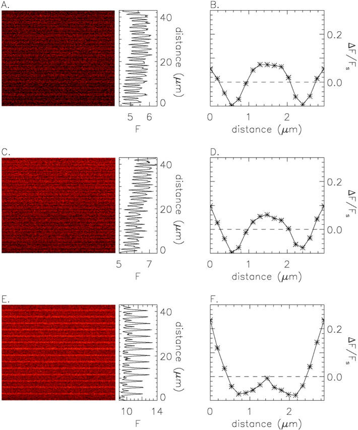
A is an F(x,t) image from a fiber from R. pipiens in normal Ringer's, and C and E are F(x,t) images from a fiber from R. temporaria in normal Ringer's and 30 mM [K⁺] Ringer's, respectively. The x axis is vertical, and the time axis is horizontal and extends 512 ms. The vertically oriented traces at the right of each panel, which show F(x), have mean values of 5.41, 6.26, and 10.47 counts/μs (A, C, and E, respectively). B, D, and F show (ΔF/F_S)(x), the normalized average sarcomeric fluctuation in F(x) (see text); distance on the abscissa runs from m-line to m-line. Fiber references, z083000b (A) and z082499b (C and E); times after injection, 25, 46, and 59 min (A, C, and E, respectively). For fiber z082499b, the change to 30 mM [K⁺] Ringer's occurred at 53 min. The images in C and E were taken at virtually identical fiber locations, 280 μm along the fiber axis from the injection site and 6 μm above the bottom surface of the fiber.

To better reveal the details of the sarcomeric periodicity, the F(x) pattern of Fig. 3 A was partitioned at m-line boundaries and the intensity data from the 14 sarcomeres were averaged. Fig. 3 B shows the result displayed in normalized units. The abscissa represents distance from one m-line to the next (sarcomere length, 2.96 μm) and the ordinate, denoted (ΔF/F_S)(x), was calculated as (F_S(x) − F_ave)/F_ave, where F_S(x) is the sarcomere-averaged F(x) pattern and F_ave is the average value of F_S(x). ΔF/F_S has a broad plateau in its middle, which contains the z-line at its center (at 1.48 μm on the abscissa), and reaches a peak value of ∼0.075. The leftmost and rightmost locations, which mark the m-lines, define a secondary maximum that reaches a peak value of ∼0.050. The minima of (ΔF/F_S)(x) are located ∼0.9 μm on either side of the z-line and have an average value of about −0.10.

A sarcomeric periodicity in F(x) has also been found in cut fibers (Tsugorka et al. 1995; Klein et al. 1996; Lacampagne et al. 1996; Shirokova and Ríos 1997). Surprisingly, in cut fibers, z-lines are centered at minima in F(x) rather than at maxima (Fig. 3 A). As mentioned below, F(x) patterns similar to those reported in cut fibers can be seen in intact fibers under some circumstances. Sarcomeric periodicities in F(x) probably occur because most of the fluo-3 molecules in myoplasm (∼85% in intact fibers) are not freely diffusible but are bound to proteins (Harkins et al. 1993; Zhao et al. 1996). Because fluo-3 likely binds to both soluble and structural proteins, we presume that sarcomeric periodicities in F(x) are due to the binding of fluo-3 to structural proteins of the sarcomere or to other proteins that can associate with structural components.

The middle two panels in Fig. 3 show results from a second fiber in normal Ringer's (this time from R. temporaria). The results are generally similar to those of the top panel. The main difference is that the amplitude of the broad plateau in (ΔF/F_S)(x) containing the z-line is slightly smaller, rather than slightly larger, than the narrow maximum marking the m-lines. Resting patterns similar to those illustrated in the top and middle panels of Fig. 3 were commonly observed in fibers from both species in normal Ringer's (see also Fig. 2 A). Within the same fiber, variations in the resting pattern were common, similar to the variation illustrated by the top and middle panels of Fig. 3.

In some fibers and images, the value of ΔF/F_S at the m-line was substantially larger than that at the z-line and the broad plateau of fluorescence centered at the z-line was absent. A pattern of this type was occasionally seen in fibers in normal Ringer's but was more frequently seen in fibers in elevated [K⁺] Ringer's. An extreme example is illustrated in the bottom two panels of Fig. 3. These data were obtained from the same fiber used for the middle panel, a few minutes after the solution bathing the fiber had been changed from normal Ringer's to 30 mM [K⁺] Ringer's. A comparison of the middle and bottom panels reveals two obvious effects of the solution change: (1) an increase of 65–70% in the mean value of F(x) (compare amplitude of F(x) traces to the right of C and E), and (2) a dramatic change in the shape of (ΔF/F_S)(x) (D and F). The new (ΔF/F_S)(x) pattern has a very prominent m-line maximum that exceeds the small peak at the z-line by ∼0.25 ΔF/F_S units. The increase in mean F(x) is expected because the depolarization produced by 30 mM [K⁺] Ringer's should elevate [Ca²⁺]_R and hence F(x). Although the change in shape of (ΔF/F_S)(x) was unexpected, it is interesting that the profile in elevated [K⁺] Ringer's is similar to that in normally polarized cut fibers (see above). This raises the possibility that the value of [Ca²⁺]_R in normally polarized cut fibers is larger than that in intact fibers. Intermediate (ΔF/F_S)(x) profiles were obtained with smaller increases in solution [K⁺], 7.5–13 mM (not shown). These changes in ΔF/F_S usually reversed after return to normal Ringer's.

Spark Detection and Frequency

In fibers in normal Ringer's, the majority of x-t images revealed either zero or one spark. In contrast, in 13 mM [K⁺] Ringer's, the majority of images revealed two or more sparks. The likely cause of this increase in spark frequency is the more positive value of membrane potential associated with the higher [K⁺] (Hodgkin and Horowicz 1959) and its ability to activate t-tubular voltage sensors, which in turn activate sparks (Tsugorka et al. 1995; Klein et al. 1996). The mean spark frequency in 13 mM [K⁺] Ringer's (estimated membrane potential, −60 to −65 mV) exceeded that in normal Ringer's (estimated membrane potential, −80 to −90 mV) by an order of magnitude (see below). Thus, it is likely that most sparks detected in 13 mM [K⁺] Ringer's were voltage-activated sparks.

Fig. 4 shows images from a fiber that was bathed successively in normal Ringer's (left), 13 mM [K⁺] Ringer's (center), and normal Ringer's (right). The top panels show F(x,t) images in the three solutions (pseudocolor scale not shown), and the bottom panels show the same images after conversion to ΔF/F units (see Fig. 5 for amplitude calibrations). The images were analyzed for sparks by the automatic detection routine described in materials and methods (detection threshold, ΔF/F = 0.3). No sparks were detected in either image in normal Ringer's but nine sparks were detected in the image in 13 mM [K⁺] Ringer's. These sparks were distributed among six different sarcomeres and each spark was centered on a z-line (midway between adjacent narrow peaks in the F(x,t) image, which mark m-lines; see Fig. 3). The vertical arrowheads at the bottom of the middle panel identify the time of the two largest sparks (discussed below in connection with Fig. 5).

Figure 4.

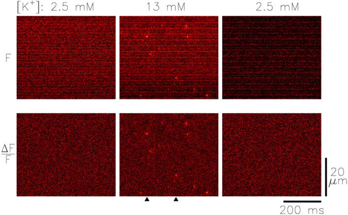
x-t images from a fiber from R. pipiens taken at similar fiber locations in normal Ringer's (left and right) and 13 mM [K⁺] Ringer's (center). The top row of images are in fluorescence intensity units and the lower row in normalized units (ΔF/F; pseudocolor scales not shown). The mean intensity levels were 3.01, 4.61, and 2.43 counts/μs, and the times after injection were 32, 39, and 107 min (left, center, and right, respectively). Fiber reference, z080200a.

Figure 5.

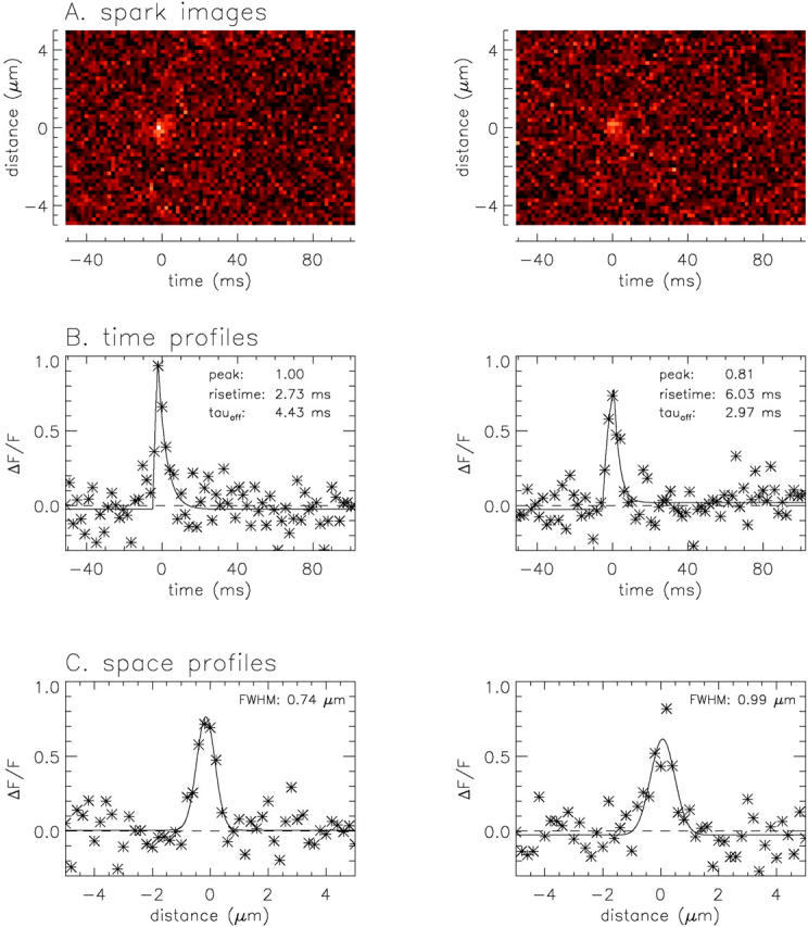
(A) Zoomed images of the two largest sparks identified in Fig. 4. (B) Asterisks show time profiles, obtained as the average of the three time lines at, and on either side of, the spatial center of the spark. Lines show least-squares fits of to the data. (C) Asterisks show space profiles, obtained as the average of two spatial lines, one just before and one just after the fitted time to peak of the spark. Lines show least-squares fits of to the data. In B and C, the dashed lines show the baselines; the values of the morphological parameters not printed on the figures are as follows: FDHM, 4.66 and 6.31 ms (left and right, respectively); late offset, 0.00 and 0.05; mass, 0.49 and 0.95 μm³. The values of peak amplitude, late offset and mass do not reflect the F′/F scaling (see text). For the nine sparks identified in Fig. 4, the mean ± SEM values of the morphological parameters (not including F′/F scaling) were as follows: rise time, 4.66 ± 0.71 ms; peak amplitude, 0.80 ± 0.05; decay time constant, 3.41 ± 0.63 ms; FDHM, 5.51 ± 0.71 ms; late offset, 0.02 ± 0.01; FWHM, 0.98 ± 0.09 μm; mass, 1.16 ± 0.40 μm³.

An important question concerning sparks is whether their distribution among sarcomeres is random. This issue is examined in a later section of results.

The protocol of Fig. 4 was performed in 10 of the 15 experiments from R. pipiens and in 1 of the 12 experiments from R. temporaria. In several of the remaining experiments, similar measurements were made either without a bracketing series of measurements in normal Ringer's or in Ringer's solutions that contained 7.5–10 mM [K⁺] instead of 13 mM [K⁺]. Table (R. pipiens) and Table (R. temporaria) give information about these experiments, including the values of [K⁺] (column 2), the times in the different solutions (column 3), the total number of detected sparks (column 5), and the average frequencies of sparks (column 6). Although the spark frequency in any particular solution appeared to be stable, a comparison of frequencies in experiments that had both initial and final bracketing measurements in normal Ringer's suggests that, on average, spark frequency may have been increasing slowly with time. For example, for R. pipiens, the initial and final spark frequencies were 0.048 ± 0.014 and 0.102 ± 0.026 sarcomere⁻¹ s⁻¹, respectively (mean ± SEM, N = 10; calculated from column 6 in Table ). For R. temporaria, the corresponding frequencies were 0.069 ± 0.026 and 0.081 ± 0.035 sarcomere⁻¹ s⁻¹ (N = 3; column 6 of Table ). Although neither of these differences between initial and final frequencies is statistically significant, in both cases the second mean frequency is larger than the first.

Table 1.

Spark Frequencies in R. pipiens (Continued)

1	2	3	4	5	6
Fiber No.	Ringer [K+]	Time	F′/F	No. of sparks	Frequency
	mM	min			sarcomere−1 s−1
z072600a	2.5	11		6	0.024
	13	19	1.30	379	0.662
	2.5	9		1	0.055 (2.29)
z072600b	2.5	9		23	0.104
	13	39	1.43	947	1.012
	2.5	10		63	0.215 (2.07)
z073100aa	2.5	14		41	0.121
	13	56	1.37	477	1.021
	2.5	12		75	0.252 (2.08)
z080200aa	2.5	9		1	0.003
	13	60	1.30	510	0.556
	2.5	18		23	0.069 (23.0)
z080800a	2.5	9		0	0.000
	13	27	1.29	178	0.403
	2.5	37		0	0.000
z080800ba	2.5	10		3	0.010
	13	36	1.26	52	0.168
	2.5	14		22	0.061 (6.10)
z081800bb	2.5	18		35	0.096
	13	44	1.23	262	0.510
	2.5	9		22	0.085 (0.88)
z082300ab	2.5	10		6	0.023
	13	68	1.38	339	0.423
	2.5	17		75	0.162 (7.04)
z082300b	2.5	8		1	0.004
	13	32	1.08	8	0.030
z082800ab	2.5	8		17	0.062
	13	41	1.34	492	0.893
	2.5	9		6	0.034 (0.55)
z082800bb	2.5	7		9	0.038
	13	58	1.68	1,057	1.545
	2.5	11		31	0.086 (2.26)
z083000a	2.5	9		3	0.009
	13	13	1.64	293	0.711
z083000b	2.5	10		21	0.066
	13	11	1.26	286	0.804
z090700a	2.5	13		36	0.091
z090700b	2.5	10		34	0.109
	13	11	1.25	243	0.679
Mean ± SEM	2.5 (N = 15)	20.1 ± 2.6		37 ± 9	0.069 ± 0.014
	13 (N = 14)	36.8 ± 5.1	1.34 ± 0.04	395 ± 80	0.673 ± 0.102

Column 1 gives the fiber identification; column 2, the value of [K⁺]; column 3, the time in each [K⁺] solution; column 4, the ratio of resting fluorescence in elevated [K⁺] Ringer's (F′) to that in 2.5 mM [K⁺] Ringer's (F); column 5, the number of sparks detected in each solution; column 6, the spark frequency (equal to the number of sparks detected in each solution divided by the product of the number of sarcomeres studied times the total recording time for the images in that solution). For fibers that had measurements at early and late times in Normal Ringer's, the number in parentheses in column 6 gives the ratio of spark frequencies for the late and early exposures. Where possible, the value in column 4 was obtained from the average of two F′/F values: that estimated for the change from Normal Ringer's to elevated [K⁺] Ringer's and that for the change back to Normal Ringer's. For the calculation of the mean ± SEM values in the bottom row, a mean value for each solution (2.5 and 13 mM [K⁺] Ringer's) was first obtained for each experiment and these values were then averaged. Fiber numbers marked with superscript b and a denote experiments that contributed to the measurements summarized in Table and Table , respectively. Sarcomere length, 3.00 ± 0.06 μm.

Table 2.

Spark Frequencies in R. temporaria

1	2	3	4	5	6
Fiber No.	Ringer [K+]	Time	F′/F	No. of sparks	Frequency
	mM	min			sarcomere−1 s−1
z051899c	2.5	16		6	0.024
z052099a	2.5	20		46	0.149
z052599a	2.5	9		9	0.042
	7.5	16	1.15	48	0.176
	2.5	14		10	0.039 (0.93)
z052599b	2.5	11		29	0.120
	10	9	1.23	34	0.190
	2.5	20		53	0.150 (1.25)
z082499b	2.5	18		3	0.008
z111899a	2.5	4		0	0.000
z112399a	2.5	5		1	0.006
z112499b	2.5	4		0	0.000
z120399a	2.5	4		4	0.046
z120999a	2.5	11		5	0.019
z052000b	2.5	8		4	0.012
	10	9	1.14	8	0.036
z052600a	2.5	9		9	0.044
	13	24	1.31	177	0.261
	2.5	16		24	0.054 (1.23)
Mean ± SEM	2.5 (N = 12)	14.1 ± 2.7		14.4 ± 7.2	0.041 ± 0.015
	13 (N = 1)	24	1.31	177	0.261

Presentation is the same as Table . Sarcomere length, 3.02 ± 0.05 μm.

For the 10 fibers from R. pipiens in which the protocol of Fig. 4 was used, the mean spark frequency in 13 mM [K⁺] Ringer's was 0.719 ± 0.127 sarcomere⁻¹ s⁻¹; in contrast, the average of the initial and final bracketing frequencies in normal Ringer's was 0.075 ± 0.019 sarcomere⁻¹ s⁻¹. For the four fibers from R. pipiens that had no final bracketing measurement in normal Ringer's, the mean frequencies were 0.556 ± 0.177 and 0.047 ± 0.025 sarcomere⁻¹ s⁻¹ in 13 mM [K⁺] Ringer's and normal Ringer's, respectively. Both of these differences are highly statistically significant and indicate that the frequency in 13 mM [K⁺] Ringer's is ∼10-fold larger than that in normal Ringer's.

For the single experiment from R. temporaria in which the protocol of Fig. 4 was used, the frequency in 13 mM [K⁺] Ringer's was about fivefold larger than that in normal Ringer's, 0.261 vs. 0.049 sarcomere⁻¹ s⁻¹. For the experiments with intermediate [K⁺] (7.5–10 mM; Table ), spark frequencies were generally intermediate between the values measured in normal and in 13 mM [K⁺] Ringer's.

The first spark measurements in elevated [K⁺] Ringer's were usually made 1–2 min after the solution change. In contrast, in voltage-clamp experiments on cut fibers, measurements are usually made during the first second after a depolarization. Spark frequencies immediately after depolarization in elevated [K⁺] Ringer's might be somewhat different from the values given in Table Table .

The 10-fold increase in spark frequency upon depolarization with 13 mM [K⁺] Ringer's is probably a lower limit because of missed sparks in the 13 mM [K⁺] Ringer's. This happens because [Ca²⁺]_R and therefore resting F increase with depolarization. On average, exposure to 13 mM [K⁺] Ringer's increased F by ∼1.3 (F′/F, Table and Table , column 4), implying a roughly similar increase in [Ca²⁺]_R. Because the associated increase in [Ca²⁺]_R is expected to have little effect on the amplitude of ΔF produced by an SR Ca²⁺ release event of fixed amplitude and duration (unpublished theoretical analysis), the value of the ΔF/F is expected to be reduced by ∼1.3-fold. As a result, fewer sparks would be detected by our autodetection program in 13 mM [K⁺] Ringer's.

Estimation of Morphological Parameters

For further analysis, it is important to have a quantitative characterization of the temporal and spatial features of sparks. Fig. 5 A shows zoomed ΔF/F images of the two largest sparks identified in the middle panel of Fig. 4. Both sparks have a similar appearance. In Fig. 5B and Fig. C, the asterisks show extracted time and space profiles, respectively, of these sparks, and the curves show the least-squares fits of and to the profiles (materials and methods). From the fits, estimates were obtained for the main morphological parameters considered below: rise time, peak amplitude, decay time constant, FDHM, late offset, FWHM, and mass (see Fig. 5 and legend for information on the fitted values of these and other sparks in Fig. 4).

Because [Ca²⁺]_R and consequently resting fluorescence was larger in elevated [K⁺] Ringer's than in normal Ringer's (see preceding section), ΔF/F amplitudes of sparks measured in 13 mM [K⁺] Ringer's were scaled by the factor 1.3 (= F′/F) for subsequent analysis to make these amplitudes comparable to those measured in normal Ringer's. For example, after the 1.3-fold scaling, the amplitudes of the two sparks analyzed in Fig. 5 are 1.30 and 1.05 instead of 1.00 and 0.81. For sparks in 10 and 7.5 mM [K⁺] Ringer's, fitted amplitudes were scaled by smaller factors, 1.2 and 1.1, respectively (Table , column 4). With these corrections, sparks produced in the different solutions by similar Ca²⁺ release events are expected to have similar ΔF/F amplitudes.

(Note: for several reasons, the F′/F correction procedure provides only an approximate method for the comparison of ΔF/F amplitudes in solutions with different [K⁺]. First, in some but not all experiments, the value of F′/F varied somewhat with time, being larger for the change from normal to elevated [K⁺] Ringer's than for the change from elevated [K⁺] back to normal Ringer's. Second, at any particular [K⁺], there was undoubtedly some fiber to fiber variation in [Ca²⁺]_R and, therefore, in the resting fluorescence intensity per unit concentration of fluo-3. Third, it is possible that other factors, such as the degree of Ca²⁺ loading of the SR, may have contributed to fiber to fiber variation in spark amplitudes.)

Table gives the mean values of the morphological parameters of sparks in normal Ringer's and in elevated [K⁺] Ringer's for the fibers from R. pipiens and R. temporaria. For two reasons, the data in the Table were restricted to “larger” sparks, defined as sparks with a fitted peak amplitude of at least 0.7 ΔF/F (after F′/F scaling). First, with larger sparks, estimates of morphological parameters are influenced less by photon and instrumentation noise. Second, larger sparks are likely to have been detected with a similar, high probability in both elevated [K⁺] and normal Ringer's. (In contrast, smaller release events are less likely to have been detected in elevated [K⁺] Ringer's than in normal Ringer's because of the difference in resting F and hence ΔF/F; see final paragraph of preceding section.)

Table 3.

Properties of Larger Sparks in Normal Ringer's and Elevated [K⁺] Ringer's

	1		2	3
R. pipiens
	Morphological parameter	Units	Normal Ringer's (N = 237)	13 mM [K+] Ringer's (N = 3,176)
	0–100% rise time	ms	3.70 ± 0.09	4.18 ± 0.03a
	Peak amplitude	ΔF/F	1.06 ± 0.03	1.08 ± 0.01
	Decay time constant	ms	4.32 ± 0.13	4.60 ± 0.04
	FDHM	ms	5.37 ± 0.11	5.92 ± 0.04a
	Late offset	ΔF/F	0.013 ± 0.002	0.013 ± 0.001
	FWHM	μm	0.95 ± 0.02	1.02 ± 0.01a
	Mass	μm3	1.65 ± 0.14	1.94 ± 0.05
R. temporaria
	Morphological parameter	Units	Normal Ringer's (N = 69)	7.5–13 [K+] Ringer's (N = 132)
	0–100% rise time	ms	3.49 ± 0.15	4.10 ± 0.14a
	Peak amplitude	ΔF/F	0.92 ± 0.02b	0.84 ± 0.01a,b
	Decay time constant	ms	4.92 ± 0.30b	5.05 ± 0.23b
	FDHM	ms	5.66 ± 0.23	6.18 ± 0.17a
	Late offset	ΔF/F	0.014 ± 0.005	0.014 ± 0.005
	FWHM	μm	0.95 ± 0.04	0.99 ± 0.03
	Mass	μm3	1.28 ± 0.17	1.35 ± 0.13a

Entries show mean ± SEM values for sparks with a fitted peak amplitude ≥0.7 ΔF/F. All data were obtained with a line scan period of 2.048 ms. ^aSignificant difference (at P < 0.05) between the mean values of columns 2 and 3. ^bSignificant difference between the corresponding mean values for R. temporaria and R. pipiens. The number of fibers were 15 (column 2) and 14 (column 3) for R. pipiens and 12 (column 2) and 4 (column 3) for R. temporaria (see Table and Table ). As described in the text, ΔF/F values in column 3 were corrected by the F′/F scaling procedure, with F′/F factors of 1.3, 1.2, and 1.1 (13, 10, and 7.5 mM [K⁺] Ringer's, respectively). For the sparks from R. pipiens in 13 mM [K⁺] Ringer's, the average value of spark amplitude from the 14 individual experiments ranged from 0.87 to 1.26 (mean ± SEM = 1.06 ± 0.03; N = 14). Temperature: 17–19°C for R. pipiens, 17–20°C for R. temporaria.

The mean morphological parameters in Table characterize the basic properties of sparks in amphibian intact fibers under these experimental conditions. Although the parameters are quite similar for the two species and the two recording solutions, there are some small but significant differences. A superscript a (^a) in column 3 of Table identifies a morphological parameter with a mean value that is significantly different in normal and elevated [K⁺] Ringer's. For R. pipiens, three parameters were slightly larger in 13 mM [K⁺] Ringer's than in normal Ringer's. The percent increases are as follows: 13% for rise time, 10% for FDHM, and 7% for FWHM. For R. temporaria, rise time and FDHM were also slightly larger in elevated [K⁺] Ringer's (by 17% and 9%, respectively), although FWHM was not significantly different. Peak amplitude was slightly smaller in elevated [K⁺] Ringer's (by 9%).

For both R. pipiens and R. temporaria, the largest significant parameter difference is for rise time (13–17% larger in elevated [K⁺] Ringer's). This difference may arise because the rate of voltage-sensor deactivation at the membrane potential of normal Ringer's is faster than that of elevated [K⁺] Ringer's (Lacampagne et al. 2000).

We also looked for significant differences between sparks in fibers from R. pipiens and R. temporaria. A superscript b (^b) in Table indicates a statistically significant difference between species. The mean values of peak amplitude and decay time constant were significantly different in both normal and elevated [K⁺] Ringer's, whereas the mean spark mass was significantly different only in elevated [K⁺] Ringer's. Spark amplitude was 15–30% larger, mass was 30–45% larger, and decay time constant was 10–15% smaller in R. pipiens than in R. temporaria. Interestingly, the peak value of ΔF/F elicited by an action potential (measured on the optical bench apparatus a few minutes after the fluo-3 injection; materials and methods) was 40–50% larger in R. pipiens than in R. temporaria (see first section of results). Although the underlying reason(s) for all of these differences is not clear, the larger spark amplitude (and consequently spark mass) in R. pipiens may be due to a smaller value of [Ca²⁺]_R.

Spark Properties with a Line Scan Period of 1 ms

The data in Table were obtained with the standard line scan period of this study, 2.048 ms (materials and methods). Because the mean value of spark rise time (∼4 ms) is only about twice the scan period, the rising phase of the spark was not well resolved; consequently, estimates of rise time may have some systematic error. To test for this possibility, four experiments were performed with line scan periods of both 1 and 2 ms. Fibers were bathed in 13 mM [K⁺] Ringer's to induce sparks and three sets of images were recorded: first with a line scan period of 2.048 ms, then with 1.024 ms, and then again with 2.048 ms. With the 1.024-ms scan period, it was necessary to reduce the excursion of the scan mirror from a useful length of 43.0 μm at the fiber to 17.3 μm. Both this reduction and the shorter scan period decreased the mean number of sparks detected per image. In each experiment, the spark frequency (units of sarcomere⁻¹ s⁻¹) was similar during the three recording periods. Fig. 6 and Fig. 7 give examples of the images recorded and morphological fits obtained in these experiments. Table summarizes the morphological parameters tabulated by scan period; the values from the initial and final sets of measurements with the 2.048-ms scan period were similar (not shown). Although the mean parameter values from the two scan periods are quite similar, four of the six means are statistically different (indicated by superscript a; column 3). In each case, the mean value with the 2.048-ms scan period is slightly larger than that with the 1.024-ms scan period; the percent increases are 15% for rise time, 8% for FDHM, 9% for FWHM, and 33% for mass.

Figure 6.

F(x,t) images from a fiber from R. pipiens in 13 mM [K⁺] Ringer's, with line scan periods of 2.048 ms (left) and 1.024 ms (right). The vertically oriented traces at the right show F(x), the spatial profile of fluorescence, obtained as the time average of F at each spatial location after exclusion of pixels that were part of identified sparks. (On the left, the peak in F(x) at ∼11.5 μm is due to a faint streaker; Fig. 2). The images were taken 47 min (left), 18 min (top right), and 41 min (bottom right) after introduction of the 13 mM [K⁺] Ringer's. Fiber reference, z082800b.

Figure 7.

Zoomed images (A; in ΔF/F units) with fits (B and C) of the two largest sparks identified in Fig. 6 (time of spark occurrence: ∼150 ms in the left-hand image of Fig. 6 and ∼55 ms in the lower right-hand image of Fig. 6). In B and C, the values of the fitted parameters not printed on the figure are as follows: FDHM, 5.47 and 5.28 ms (left and right, respectively); late offset, 0.06 and 0.01; mass, 1.42 and 1.69 μm³. Values of peak amplitude, late offset, and mass do not include F′/F scaling (see text).

Table 4.

Properties of Larger Sparks with 1- and 2-ms Scan Periods

1		2	3
Morphological parameter	Units	1.024-ms scans (N = 358)	2.048-ms scans (N = 876)
0–100% rise time	ms	3.60 ± 0.09	4.13 ± 0.07
Peak amplitude	ΔF/F	1.09 ± 0.02	1.13 ± 0.01
Decay time constant	ms	4.84 ± 0.11	4.93 ± 0.08
FDHM	ms	5.67 ± 0.11	6.13 ± 0.08
Late offset	ΔF/F	0.010 ± 0.002	0.015 ± 0.002
FWHM	μm	0.93 ± 0.02	1.01 ± 0.01
Mass	μm3	1.42 ± 0.08	1.89 ± 0.09

Entries show mean ± SEM values for sparks from R. pipiens with a fitted peak amplitude ≥ 0.7 ΔF/F, measured with 1.024- and 2.048-ms scan periods (columns 2 and 3, respectively). The data were collected in 13 mM [K⁺] Ringer's from the four fibers marked by a superscript b in column 1 of Table . As in Table , ΔF/F amplitudes were corrected by the F′/F scaling procedure (factor = 1.3). Temperature, 17–19°C.

Numerical analysis of simulated sparks (not shown) was also used to evaluate possible errors in the estimation of morphological parameters with the 2-ms scan period. The time course of simulated sparks was assumed to satisfy . Random noise was added to the waveform to approximate the photon noise in the measurements. Variability was also introduced to simulate uncertainty in the time of spark onset relative to spark sampling (uncertainty assumed to be distributed uniformly between ± 0.5 time pixels). The analysis indicated that, if the actual spark rise time is 4 ms, the use of a 2-ms line scan period overestimates mean rise time by ∼5%; if the actual rise time is 3 ms, the overestimate is ∼20%. With a 1-ms scan period, the overestimates are smaller, 0 and 5%, respectively. These results are in reasonable agreement with the results in Table , where the mean rise time with the 2-ms scan period is ∼15% larger than that with the 1-ms scan period. The combined results of Table and the numerical analysis support the conclusion that the rise times in Table and Table are reasonably accurate, although the values obtained with the 2-ms scan period may be overestimated by 10–20% if the actual spark waveform is accurately described by the theoretical spark waveform.

Spark Properties with y-t Scanning

In the experiments described above, the spatial spread of a spark was measured in only the x direction (along the fiber axis). In cardiac myocytes, however, the spatial spread of a spark depends on direction; at the time of the peak of a spark, FWHM in y (the direction perpendicular to the fiber axis and to the light path) is 15% (Cheng et al. 1996) to 30% (Parker et al. 1996) smaller than that in x. To test for this possibility in our experiments, sparks were measured with x-t and y-t scanning (2.048-ms scan period) in three fibers bathed in 13 mM [K⁺] Ringer's to induce sparks. In each experiment, three sets of images were recorded: first, with the chamber in its normal orientation; second, with the chamber rotated by 90°; and, third, again in the normal orientation. Spark frequency was similar during the three recording periods, as were the average morphological parameters estimated from the initial and final sets of x-t measurements. Fig. 8 shows examples of x-t and y-t images recorded in these experiments. The y-t images showed no obvious sign of spark synchronization in the y direction, which contrasts with the situation reported for rat cardiac myocytes (Parker et al. 1996). Fig. 9 shows zoomed images of two sparks from Fig. 8 and their morphological fits.

Figure 8.

Fluorescence intensity images and F profiles from a fiber from R. pipiens in 13 mM [K⁺] Ringer's taken with x-t (left) and y-t (right) scanning. The images were taken 12 min (left) and 35 min (right) after introduction of the 13 mM [K⁺] Ringer's. Fiber reference, z080200a.

Figure 9.

Zoomed images (A; in ΔF/F units) with fits (B and C) of the two largest sparks identified in Fig. 8 (time of spark occurrence: ∼275 ms and ∼80 ms in the left and right-hand images, respectively, of Fig. 8). In B and C, the values of the fitted parameters not printed on the figure are as follows: FDHM, 5.19 and 5.62 ms (left and right, respectively); late offset, -0.03 and 0.01. Values of peak amplitude and late offset do not include F′/F scaling (see text).

Table presents a summary of the morphological parameters obtained from the x-t and y-t images (columns 2 and 3, respectively). Only the values of FWHM are statistically significantly different and the difference is only 6%. These results support the conclusion that the diffusion of free Ca²⁺, fluo-3, and the other mobile Ca²⁺ buffers that affect the spatial spread of a spark occurs almost isotropically in frog myoplasm. Brum et al. 2000, working in cut fibers, also found that the spatial spread of sparks is very similar in x and y (if measured in the absence of caffeine).

Table 5.

Properties of Larger Sparks with x-t and y-t Scanning

1		2	3
Morphological parameter	Units	x-t scanning (N = 687)	y-t scanning (Ν= 653)
0–100% rise time	ms	4.13 ± 0.07	4.00 ± 0.06
Peak amplitude	ΔF/F	1.08 ± 0.01	1.08 ± 0.01
Decay time constant	ms	4.55 ± 0.09	4.56 ± 0.09
FDHM	ms	5.85 ± 0.08	5.75 ± 0.07
Late offset	ΔF/F	0.011 ± 0.002	0.014 ± 0.002
FWHM	μm	1.03 ± 0.01	0.97 ± 0.01a

Entries show mean ± SEM values for sparks from R. pipiens with a fitted peak amplitude ≥0.7. The data were collected in 13 mM [K⁺] Ringer's from the three fibers marked by a superscript a in column 1 of Table . As in Table , ΔF/F amplitudes were corrected by the F′/F scaling procedure (factor = 1.3). All data were obtained with a line scan period of 2.048 ms. Temperature, 17–19°C.

^aSignificant difference between means in columns 2 and 3.

Late ΔF/F Phase of a Spark

In their study of sparks in cut fibers, Gonzalez et al. 2000b reported the existence of an “ember,” a small, long lasting fluorescence increase that can be detected in an average x-t image formed from a large number of voltage-activated sparks. 28–48 ms after the peak, this late ΔF/F signal had an amplitude of 0.1–0.2 (relative to the prespark baseline) and a FWHM of ∼1 μm.

To determine the properties of such late signals in intact muscle fibers, an average x-t image was formed from 1,767 sparks recorded in 13 mM [K⁺] Ringer's and aligned at the time of peak. Fig. 10 A shows the average F(x,t) image displayed at high gain. This image reveals the average spark superimposed on the average resting fluorescence pattern. The F(x) signal from the prespark period is shown at the left, where the tall narrow peaks mark m-lines. As expected, the average spark is highly symmetric about the central z-line. Fig. 10B and Fig. C, show ΔF/F images of the average spark at low and high gain, respectively (see Fig. 11 for amplitude calibrations).

Figure 10.

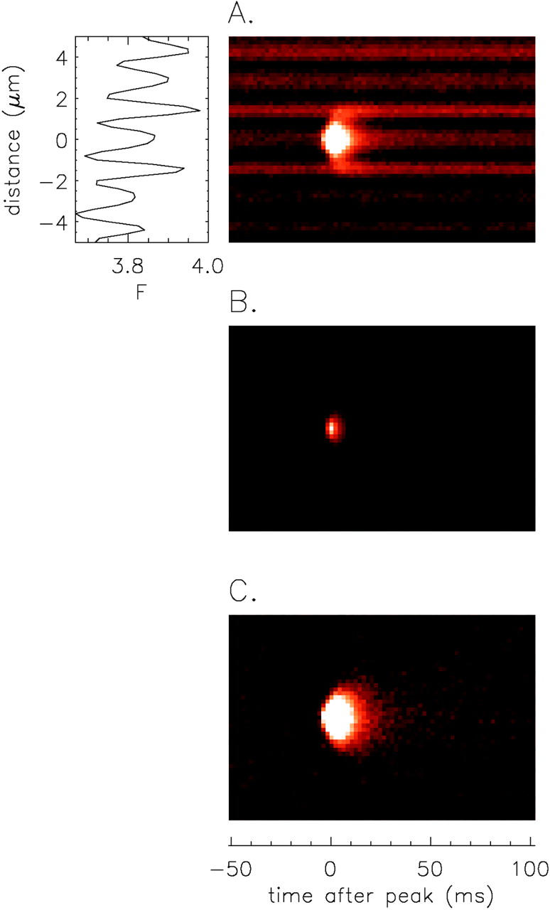
Average x-t images (10.2 μm by 155.6 ms) obtained from 1,767 sparks from R. pipiens in 13 mM [K⁺] Ringer's (line scan period, 2.048 ms). All analyzed and accepted sparks (materials and methods) were included in the average if (1) rise time was 2–7 ms; (2) amplitude was ≥ 0.7 ΔF/F; (3) no other sparks occurred at the same z-line during the 155.6-ms image period; and (4) a full x-t sub-image containing the spark (10.2 μm by 155.6 ms) was recorded. [Note: the positive late baseline offset criterion (A₂ < 0.15; see materials and methods) led to rejection of only one spark from the average.] All sparks were aligned so that the nearest pixel to the fitted time of peak always occurred at t = 0 ms and the nearest pixel to the fitted center of the spark occurred at x = 0 μm. (A) Average F(x,t) image displayed at a high gain to reveal the sarcomeric resting fluorescence pattern, F(x); most of the central pixels of the average spark are in saturation due to the high display gain (see Fig. 11 for amplitude of ΔF/F). The F(x) trace to the left is the average of the first 20 line scans (t < −10 ms); the narrow peaks mark m-lines. (B and C) Average ΔF/F images calculated from the F(x,t) image and the F(x) profile in A. In B, the (ΔF/F)(x,t) image is displayed at low gain; in C, the image is redisplayed at fivefold higher gain to reveal a possible “ember” (see text and Fig. 11).

Figure 11.

Data and fits from the ΔF/F image of Fig. 10; all amplitudes reflect the F′/F scaling procedure (factor = 1.3). (A) Asterisks show single temporal profile from the central z-line (x = 0 μm). The curve is the fit of , which gave the following parameter values: rise time, 4.55 ms; peak amplitude, 0.97; decay time constant, 5.19 ms; FDHM, 6.56 ms; and late offset, 0.014. Squares show the average temporal profile from the two immediately adjacent m-lines (3 profiles from each m-line). (C) Asterisks indicate single spatial profile at the time to peak of the spark (t = 0 ms); squares average of the 10 spatial profiles recorded during the period 28–48 ms after the spark peak. The curve is the fit of to the asterisk data; the fit gave values of 0.99 for peak amplitude and 0.96 μm for FWHM. (E) Square data of panel C displayed at higher vertical gain. The fit of (curve) gave values of 0.018 for peak amplitude and 2.94 μm for FWHM. (B and D) Values of amplitude (B) and FWHM (D) obtained from fits of to spatial profiles at different times (C with E). The fitted values of x₀ (not shown) fell in the range −0.2 to +0.3 μm. The curve in B is the same as that in A. (F) Spark mass, calculated from amplitude (B) and FWHM (D) with . In B, D, and F, squares give values obtained from fits to single line scans. To reduce noise in the small signals at later times, averages were used; triangles and circles show values obtained from fits to averages of three and nine line scans, respectively. The filled circles show the results of fitting to the average of the 10 line scans at 28–48 ms.

Fig. 11 A shows two temporal profiles extracted from the ΔF/F image of Fig. 10. The asterisks show the profile measured at the central z-line; this signal-averaged profile is much less noisy than that of a typical spark (Fig. 5 B, 7 B, and 9 B). The squares show the average of the profiles measured at the two immediately adjacent m-lines. The m-line signal has an amplitude that is ∼7% of that of the z-line signal and reaches a peak ∼4 ms after the z-line signal. The curve in Fig. 11 A shows the fit of to the z-line signal. As expected, the parameter values obtained from the fit (see legend) are close to the mean values in column 3 of Table R. pipiens.

Fig. 11 C shows two spatial profiles from the ΔF/F image of Fig. 10, one obtained at the time of peak of the spark (t = 0 ms; asterisks) and the other at the time of the late signal as studied by Gonzalez et al. 2000b (t = 28–48 ms; squares). The late profile has been replotted in Fig. 11 E at higher gain. The curves in Fig. 11 C and E show the fits of the standard Gaussian function () to these profiles. The fits yielded amplitude and FWHM values of 0.99 ΔF/F and 0.96 μm (Fig. 11 C) and 0.018 ΔF/F and 2.94 μm (Fig. 11 E). The late signal in intact fibers is substantially different from that described in cut fibers: the amplitude is ∼0.2 times that found by Gonzalez et al. 2000b and the FWHM is about three times larger.

Fig. 11 (B and D) shows the time courses of the amplitude and FWHM of ΔF/F, estimated from fits of to spatial profiles derived from Fig. 10 (as in Fig. 11C and Fig. E). The amplitude decreases progressively after the peak, as expected from Fig. 11 A, whereas the value of FWHM increases (note the different vertical gains in Fig. 11A and Fig. B). Fig. 11 F shows the time course of spark mass (). As mentioned in materials and methods, the product of spark mass times [Ffluo]_R approximates the total increase in Ca-fluo-3 (in moles) if the Ca²⁺ spark is at the scan line. Interestingly, at the time of peak of the average spark (t = 0 ms), which is thought to mark the termination of Ca²⁺ release (Cannell et al. 1995), signal mass is rising rapidly and does not reach its maximum until ∼5 ms later (two to three data points). Although the Ca²⁺ source is not centered at the scan line for all larger sparks, this increase in spark mass after the peak likely reflects increased binding of Ca²⁺ to fluo-3 after Ca²⁺ release has ceased. A delay of this type is expected because of the kinetic delay in the reaction between Ca²⁺ and fluo-3 in the myoplasmic environment (Harkins et al. 1993; Baylor and Hollingworth 1998).

Although the data in Fig. 11 B were obtained from Gaussian fits, they essentially superimpose, within the noise, the asterisk data in Fig. 11 A at t > 2 ms. The curve in Fig. 11 B is the same as that in Fig. 11 A. For 14 < t < 38 ms, the data lie above the fitted curve, whereas, for t > 46 ms, the data lie below the curve (Fig. 11 B). The discrepancy between the data and curve suggests that the falling phase of a spark contains an additional slow component. Therefore, it was of interest to refit the asterisk data of Fig. 11 A with a modified version of in which the decay of a spark follows a double-exponential (rather than a single-exponential) time course. This fit was performed both with and without the inclusion of a baseline offset. In both fits, the data were well described by a double-exponential decay. The time constant of the fast component was 4.6 ms and that of the slow component was 25–35 ms; the fractional amplitudes of the fast and slow components were 0.93 and 0.07, respectively (both fits). These results indicate that the decay phase of a spark has a small slow component whose time constant is severalfold larger than that of the large fast component, and that the positive baseline offset estimated in the fits with (Tables III–VI) reflects the presence of this slow component.

Early ΔF/F Phase of a Spark

To further explore the idea that the Ca²⁺ released by one RYR might serve as the immediate trigger of a cluster of RYRs responsible for a spark (Gonzalez et al. 2000b), we investigated whether the period immediately preceding the main rising phase of a spark reveals a fluorescence increase that might indicate a trigger signal. As shown by the asterisks in Fig. 11 A, the value of ΔF/F at the central location of the average spark is close to baseline during the prespark period (t = −50 to −4 ms). Thus, any early increase in fluorescence reflective of putative trigger activity is likely to be small. To study this further, a new average x-t image was formed, in which spark alignment was based on time of onset rather than time of peak. The voltage-activated sparks used for this new image were the same as those used for Fig. 10. The baseline used to correct the ΔF/F signal was formed from the average of the first 11 line scans in the image (t = −47 to −27 ms). Fig. 12 A shows the central time profile from this ΔF/F image.

Figure 12.

Data, and fits at early times, from an average ΔF/F image. This image used the same sparks as in Fig. 10, but spark alignment was based on time of onset rather than time of peak. (For each spark in the average, was fitted to the temporal profile and the pixel immediately preceding t = t₁ was taken as the alignment point.) (A) Asterisks indicate the temporal profile from the central z-line (x = 0 μm). The fit of (curve) gave the following values: rise time, 3.48 ms; peak amplitude, 1.05; decay time constant, 5.36 ms; FDHM, 5.89 ms; and late offset, 0.013. (B) Squares show spatial profiles at t = 0 ms (top), t = −2.048 ms (middle) and t = −4.096 ms (lower). The curves are the fits of to the data. See text for values of fitted parameters. All amplitudes reflect the F′/F scaling procedure (factor = 1.3).

To examine the onset of the spark, three spatial profiles were extracted from the average x-t image. These profiles (Fig. 12 B, squares) correspond to the scan line at the nominal time of spark onset (t = 0 ms; top profile) and to the two scan lines immediately preceding spark onset (t = −2.048 ms and t = −4.096 ms; middle and bottom profiles, respectively). The curves in Fig. 12 B are the best fits of the usual Gaussian function (). From these fits, the following values of ΔF/F and FWHM were obtained: 0.032 and 1.34 μm, 0.009 and 1.51 μm, and 0.014 and 1.50 μm, respectively. At the nominal time of spark onset (t = 0 ms), the small positive ΔF/F that is detected is ∼3% of peak. This small signal might conceivably reflect a trigger phase of ΔF/F. At t < 0 ms, the fitted values of amplitude are within the noise of the baseline (mean ± SD = 0.001 ± 0.008 ΔF/F, obtained from similar fits to the first 11 line scans); thus, a reliable signal was not detected at t < 0 ms. Overall, the small positive amplitude detected at t = 0 ms (3% of peak) implies that any trigger phase preceding a voltage-activated spark must be very small in comparison with the spark itself.

Repetitive Spark Activity within Individual Sarcomeres

Klein et al. 1999, in a study of voltage-activated sparks in cut fibers, noted that occasional images revealed repetitive sparks (“rep-mode” sparks), i.e., multiple sparks occurring at the same z-line with a frequency far greater than that expected from the average spark frequency. In our experiments, repetitive sparks were also occasionally observed. Fig. 14 A shows an example from a fiber from R. pipiens in 13 mM [K⁺] Ringer's. In this 1.571-s image of 14 sarcomeres, 11 sparks were detected, and all occurred at the same z-line (second from the top in Fig. 14 A). Of these, 10 passed the analysis criteria described in materials and methods and had a peak amplitude ≥ 0.7; consequently, they contributed to the average values in column 3 of Table R. pipiens. In this experiment, 558 sarcomeres were studied and the mean frequency of sparks with amplitude ≥0.7 was 0.25 per sarcomere per 1.571–s image. Under the hypothesis that the distribution of sparks among sarcomeres is random, the probability of finding a sarcomere with 10 or more sparks out of 558 sarcomeres is extremely low, <10⁻⁹ (calculated from the Poisson distribution with a mean frequency of 0.25; see next paragraph). Thus, sparks do not occur with a fixed probability that is equal among all sarcomeres.

Figure 14.

F(x,t) images illustrating different types of repetitive activity related to SR Ca²⁺ release. (A) Repetitive sparks. The autodetection routine identified 11 sparks in this 43 μm × 1.571–s image; mean resting F in the image was 5.8 counts/μs. All sparks occurred at the z-line located second from the top. 10 of the sparks passed the analysis criteria described in materials and methods and had a peak amplitude ≥ 0.7 ΔF/F (after F′/F scaling). The mean ± SEM values of the morphological parameters for these sparks were as follows: rise time, 3.12 ± 0.26 ms; peak amplitude, 1.12 ± 0.08 (after F′/F scaling); decay time constant, 3.78 ± 0.45 ms; FDHM, 4.41 ± 0.23 ms; late offset, −0.01 ± 0.01; FWHM, 0.94 ± 0.09 μm; mass, 1.43 ± 0.40 μm³. (B–D) Examples of sustained nonspark-like activity (see text). The sampling period and vertical extent of the images are 2.048 ms and 25.2 μm in B, and 1.024 ms and 17.3 μm in C and D. Fiber references are as follows: A, z080800b; B, z083000b; C, z082800a; D, z082800b.

To obtain some measure of the distribution of sparks among sarcomeres, the 3,176 voltage-activated sparks of R. pipiens (ΔF/F ≥ 0.7; Table , column 3) were sorted according to the number of sparks per sarcomere. The asterisks in Fig. 13 A show P_n, the fraction of sarcomeres that had n sparks per sarcomere in 1.571 s, plotted as a function of n (= 0, 1, 2,…12; 12 being the maximum number of sparks detected for any sarcomere). Fig. 13 B shows the same data plotted at higher vertical gain. The open squares in Fig. 13 (A and B) show the values of P_n expected for a random distribution of sparks among sarcomeres; these were calculated from a Poisson probability distribution constrained to match P₀, 0.65 (Fig. 13, legend). Compared with the values obtained from the Poisson probability distribution, the data reveal a deficit of sparks for n = 1 and an excess of sparks for n ≥ 2.

Figure 13.

Test for randomness in the sarcomeric distribution of sparks. The analyzed sparks (3,176; ΔF/F ≥ 0.7) were obtained from 355 1.571 s images having a total of 4,866 sarcomeres (Table R. pipiens, column 3). Asterisks show measured values of P_n and squares show values calculated from the Poisson distribution (P_n = e^−λ λⁿ/n!) with a mean frequency, λ, of 0.43. λ was calculated from the observed value of P₀ (0.65) and the relation P₀ = e^−λ. See text for the Poisson analysis underlying the open circles. A and B show the ordinate at low and high gain, respectively.

A possible reason for the difference between the asterisks and open squares in Fig. 13 is a nonuniform spatial distribution of RYRs in the y-z plane. Franzini-Armstrong et al. 1999 showed that the number of RYRs in a confocal x-t scan could vary widely in frog fibers, between 0 and ∼150. In making these estimates, the authors approximated the PSF in the y-z plane of the scan as a rectangle of size 0.5 μm in y and 1.0 μm in z. We have reanalyzed the images for frog skeletal muscle from their Fig. 5 using a rectangle of 0.2 μm in y and 0.5 μm in z, values close to those for FWHM of our measured PSF. In this analysis, ∼10% of scanned sarcomeres are estimated to have zero RYRs, the maximum number of RYRs in any scanned sarcomere is ∼80, and the mean number of RYRs per scanned sarcomere is 21. In Fig. 13, the open circles show the expected distribution for P_n calculated from our estimate of the spatial distribution of RYRs and the assumption that the number of sparks within a sarcomere follows a Poisson distribution with a mean frequency of 0.023 per 1.571 s per RYR. This is the frequency that gives the observed fraction of sarcomeres without sparks, 0.65. The open circles lie between the open squares and the experimental data (asterisks). Although a nonuniform spatial distribution of RYRs helps explain the observed number of sparks per sarcomere, there is still a deficit of sarcomeres for n = 1 and an excess for n > 2. Thus, both forms of the Poisson analysis support the conclusion that sparks do not occur with a fixed probability that is equal among all sarcomeres. For example, different sarcomeres may have different fixed probabilities or the probability of spark occurrence within one sarcomere might increase as a result of previous spark activity.

In Fig. 13 B, the observed values of P_n decrease along a smooth trajectory, with no obvious indication of a specific value of n that might be used as a threshold for identifying repetitive vs. nonrepetitive sparks. Thus, repetitive sparks of the type illustrated in Fig. 14 A may simply reflect an extreme result of an underlying mechanism that favors the recurrence of sparks at sites where sparks have already occurred.

A similar analysis (not shown) was also performed on the 237 sparks in normal Ringer's from R. pipiens (Table R. pipiens, column 2). These sparks were distributed among 192 out of a total of 4,564 sarcomeres in 334 images. Analogous to the procedure used in Fig. 13, the plot of P_n against n was compared with the two Poisson distributions calculated from the observed value of P₀, 0.96 (= (4,564 −192)/4,564). As in Fig. 13, P_n for both distributions revealed a deficit of sparks for n = 1 and an excess of sparks for n > 2. Thus, for both resting sparks and voltage-activated sparks, the results deviate from the simplest forms of the Poisson analysis.

We also explored the possibility that the values of spark morphological parameters might depend on n. The 3,176 sparks used for Fig. 13 were divided into three subgroups: (1) n = 1 (998 sparks); (2) n = 2–4 (1,564 sparks); (3) n = 5–12 (614 sparks). As shown in Table , the mean values of the parameters are similar for all three groups. As indicated by the superscript a in column 4, the small increases for rise time, peak amplitude, decay time constant, and FDHM are statistically significant. These results are generally consistent with the findings of Klein et al. 1999, who noted that the mean values of rise time, FDHM, and FWHM were very similar for repetitive and nonrepetitive sparks.

Table 6.

Properties of Larger Sparks for Different Numbers of Sparks per Sarcomere per 1.571–s Image

1		2	3	4
Morphological parameter	Units	n = 1 (N = 998)	n = 2–4 (N = 1,564)	n = 5–12 (N = 614)
0–100% rise time	ms	4.07 ± 0.06	4.21 ± 0.05	4.25 ± 0.07
Peak amplitude	ΔF/F	1.02 ± 0.01	1.09 ± 0.01	1.18 ± 0.02
Decay time constant	ms	4.45 ± 0.08	4.57 ± 0.06	4.94 ± 0.10
FDHM	ms	5.75 ± 0.06	5.93 ± 0.05	6.21 ± 0.08
Late offset	ΔF/F	0.014 ± 0.001	0.012 ± 0.001	0.009 ± 0.002
FWHM	μm	1.02 ± 0.01	1.02 ± 0.01	1.02 ± 0.02
Mass	μm3	1.87 ± 0.08	1.93 ± 0.07	2.06 ± 0.11

Entries show mean ± SEM values for the 3,176 sparks of column 3 of Table R. pipiens subdivided according to n (the number of sparks per sarcomere per 1.571–s image). The number in parentheses (N) gives the total number of sparks in each group. Temperature, 17–19°C.

Atypical Events

The vast majority of events observed in these experiments were narrowly confined in space and time, i.e., were unambiguously “sparklike” (Fig. 4 Fig. 5 Fig. 6 Fig. 7 Fig. 8 Fig. 9 Fig. 10). However, a few images revealed fluorescence increases that were different. These atypical events usually had a normal spatial spread but a duration that was unusually prolonged. Unlike streakers (Fig. 2 B), these events occurred at the same location as sparks (i.e., at z-lines), suggesting that they reflect the release of Ca²⁺ through active RYRs. Fig. 14 (B–D) shows three examples. In Fig. 14 B, the maintained activity (middle sarcomere of the image) appeared to begin as repetitive sparks but, at later times, changed to more sustained and less sparklike events. This pattern probably reflects atypical closings and reopenings of the same RYR or cluster of RYRs. Fig. 14C and Fig. D, shows sustained nonsparklike activity of long and short duration, respectively (second sarcomere from the top in each image). Although these rare events were not analyzed in detail, their presence is expected to have had negligible influence on the estimation of spark properties as given in Table Table Table Table Table Table .

DISCUSSION

This article describes the first detailed study of resting and voltage-activated Ca²⁺ sparks in frog intact skeletal muscle fibers. The use of intact muscle fibers for studies of excitation-contraction coupling is important because the physiological environment is expected to be as close to normal as is possible outside the whole animal. The experiments were performed with a home-built confocal microscope that has excellent spatial resolution. The values of FWHM of the microscope's point-spread function, 0.21 μm in x and y and 0.51 μm in z, are smaller than those from previous spark studies in frog cut skeletal fibers, 0.4–0.5 μm in x and y and 0.8–1.4 μm in z (Jiang et al. 1999; Ríos et al. 1999; Klein 2000). Good spatial resolution is obviously advantageous for resolving fluo-3 signals with a narrow spatial extent. Such signals include streakers (FWHM ≈ 0.3 μm; Fig. 2, B–D), intrasarcomeric periodicities in the resting fluorescence of fluo-3 (e.g., FWHM of m-line fluorescence ≈0.6 μm; Fig. 3), and sparks themselves (FWHM ≈1.0 μm; Tables III–VI).

Fluo-3 Resting Fluorescence

In intact fibers, F(x), fluo-3′s resting fluorescence along the fiber axis, revealed an oscillation with a well-defined substructure. In normal Ringer's, fluorescence at the m-line was usually similar to that at the z-line (Fig. 2 B and Fig. 3A and Fig. B). In elevated [K⁺] Ringer's, m-line fluorescence was usually larger than z-line fluorescence (e.g., Fig. 3 C and Fig. 10 A). This increase may be a consequence of an increase in [Ca²⁺]_R caused by the membrane depolarization in elevated [K⁺]. In cut fibers at the normal holding potential (−90 mV), m-line fluorescence is also larger than z-line fluorescence (Tsugorka et al. 1995; Klein et al. 1996; Lacampagne et al. 1996; Shirokova and Ríos 1997). This may indicate that [Ca²⁺]_R in cut fibers is larger than that in our intact fibers in normal Ringer's. In both intact and cut fibers, the presence of strong sarcomeric periodicities in F(x) is consistent with the idea that a substantial fraction of fluo-3 is bound to myoplasmic proteins (Harkins et al. 1993), including structural proteins. A possible mechanism for an effect of [Ca²⁺] on F(x) is that the binding of fluo-3 to sarcomeric proteins varies with [Ca²⁺] (Konishi et al. 1988; Harkins et al. 1993) or with other variables that may change with [Ca²⁺] ([Mg²⁺], pH, etc.).

Spark Frequency and Morphology

When the solution bathing an intact fiber was changed from normal Ringer's to 13 mM [K⁺] Ringer's, the mean spark frequency increased by about an order of magnitude and the elevation in frequency persisted at an approximately constant level for many tens of minutes. Thus, exposure of fibers to moderately elevated [K⁺] Ringer's provides a reliable method to induce voltage-activated sparks at a useful frequency for measurement. In both normal Ringer's and 13 mM [K⁺] Ringer's, a statistical analysis indicated that sparks do not occur with a fixed probability that is equal among sarcomeres (see Repetitive Spark Activity within Individual Sarcomeres).

Spark waveforms in time and space were fitted with standard functional forms ( and ) to estimate the morphological characteristics of sparks (Fig. 5, Fig. 7, and Fig. 9 and Tables III–VI). The waveforms extracted from individual sparks appeared to be well-fitted by and , although the noise in the data was sufficiently large that a systematic deviation between the data and the functional forms cannot be ruled out. In fact, two such deviations became apparent in the fits of and to the average ΔF/F that was complied from 1,767 sparks (Fig. 11). In Fig. 11 (A and B), the falling phase of ΔF/F does not exactly follow a single exponential decay to a baseline offset. Similarly, the best fit of a Gaussian function to the spatial profile of a ΔF/F at the time of peak (Fig. 11 C, curve and asterisks) reveals deviations; the fit overestimates the spark profile at half amplitude and underestimates the peak of the spark and the values at |x| ≥ 0.8 μm. These deviations are not surprising, since, as mentioned in materials and methods, and are not expected to exactly describe the time course and spatial spread of a spark.

Comparison of Spark Morphology in Intact and Cut Fibers from R. Pipiens

Sparks in frog intact fibers are remarkable for their small values of FDHM and FWHM (∼6 ms and ∼1.0 μm, respectively; Tables III–VI). Both of these values are substantially smaller than the corresponding values measured in other adult muscle preparations, such as frog cut skeletal fibers (9–15 ms and 1.3–2.3 μm; see next paragraphs), mouse enzyme-dissociated skeletal fibers (40 ms and 2.0 μm; Conklin et al. 1999), and rat cardiac myocytes (25–40 ms and 1.5–2.5 μm; e.g., Cheng et al. 1993, Cheng et al. 1996; Parker et al. 1996; Smith et al. 1998).

Table compares values of spark morphological parameters in frog intact fibers and in frog cut fibers under several conditions. Results from cut fibers are included only if the nominal value of free [Mg²⁺] was 0.5–1.0 mM, which is close to the physiological range. The ΔF/F threshold values for spark selection are indicated in parentheses after each entry in the Table. Two threshold values, 0.5 and 1.0, were used for intact fibers to allow comparison with results from cut fibers; these values are different from the 0.7 threshold used for Table Table Table Table . Columns 2 and 3 of Table give mean parameter values for voltage-activated sparks in intact and cut fibers, respectively; column 4 gives mean values for spontaneous sparks in cut fibers that were permanently depolarized by notching or saponin permeabilization.

Table 7.

Comparison of Morphological Parameters of Calcium Sparks from R. pipiens

1		2	3	4
	Units	Intact fibers	Voltage-clamped cut fibers	Permanently depolarized cut fibers
Rise time	ms	4.4 ± 0.1 (0.5)	4.7 ± 0.1 (0.4, c)	5.4 ± 0.2 (0.4, b)
		3.9 ± 0.1 (1.0)	4.8 ± 0.4 (0.6, e)	6.5 ± 0.2 (d)
				6.0 ± 0.1 (0.3, f)
				5.1–8.7 (1.0, g)
Peak amplitude	ΔF/F	0.99 ± 0.01 (0.5)	0.89 ± 0.03 (0.5, a)	0.75 ± 0.09 (0.4, b)
		1.36 ± 0.01 (1.0)	1.05 ± 0.03 (0.4, c)	1.5 (d)
			1.85 ± 0.12 (0.6, e)	0.63 ± 0.02 (0.3, f)
				1.65–1.83 (1.0, g)
Decay time constant	ms	4.9 ± 0.1 (0.5)	8.5 ± 0.4 (0.4, c)
		4.4 ± 0.1 (1.0)
FDHM	ms	6.3 ± 0.1 (0.5)	14.8 ± 0.3 (0.5, a)	9.7 ± 0.4 (0.4, b)
		5.6 ± 0.1 (1.0)	8.9 ± 0.2 (0.6, e)	11.2 ± 0.4 (d)
				13.3 ± 0.2 (0.3, f)
FWHM	μm	1.05 ± 0.01 (0.5)	1.51 ± 0.10 (0.5, a)	1.7 ± 0.1 (0.4, b)
		0.97 ± 0.01 (1.0)	1.33 ± 0.06 (0.6, e)	2.3 ± 0.1 (d)
				2.04 ± 0.04 (0.3, f)
				1.6–1.9 (1.0, g)
Spark mass	μm3	1.4 (0.5)	3.7 (0.5, a)	4.4 (0.4, b)
		1.5 (1.0)	5.2 (0.6, e)	22.5 (d)
				6.5 (0.3, f)
				9.5–15.0 (1.0, g)

Mean ± SEM values for intact fibers (this study; column 2) are compared with those from cut fibers (columns 3 and 4). Values in column 2 are for voltage-activated sparks in 13 mM [K⁺] Ringers; values in column 3 are for voltage-activated sparks studied with a Vaseline-gap voltage clamp; values in column 4 are for spontaneous sparks in fibers that were permanently depolarized by either notching with a hypodermic needle (ref. b) or chemical permeabilization with saponin (refs. d, f, and g). A number in parentheses gives the threshold value of ΔF/F used for spark acceptance and a letter identifies a reference according to the following code: a, Lacampagne et al., 1996; b, Lacampagne et al., 1998; c, Lacampagne et al., 1999; d, Klein et al., 1999; e, Gonzalez et al., 2000b; f, Shtifman et al., 2000; and g, Gonzalez et al., 2000a. Fiber conditions: intact fibers (17–19°C); cut fibers of a–d and f (20–23°C; nominal free [Ca²⁺], 0.1 μM; nominal free [Mg²⁺], 0.65 mM); cut fibers of e and g (17°C; nominal free [Ca²⁺], 0.1 μM; nominal free [Mg²⁺], 0.5 mM). Except for e and g, FWHM was determined from a Gaussian fit to the spatial profile of a spark (). Refs. e and g used a non-Gaussian method, which we estimate gives a value of FWHM that is only 0.8–0.85 times that obtained with the Gaussian method; the values of spark mass were calculated with from the corresponding mean values of peak amplitude and FWHM. In ref. g, the largest value of spark mass (15.0 μm³) is associated with the smallest value of rise time (5.1 ms) and with the largest value of FWHM (1.9 μm). For intact fibers, the mean values of mass calculated from individual sparks were 1.99 ± 0.05 (threshold, 0.5; N = 3,871) and 1.96 ± 0.06 (threshold, 1.0; N = 1,480).

The rise time of voltage-activated sparks is similar in both intact and cut fibers, 3.9–4.8 ms (columns 2–3), whereas the rise time of spontaneous sparks in permanently depolarized cut fibers is larger, 5.1–8.7 ms (column 4). At comparable detection thresholds, the amplitude of voltage-activated sparks is similar in intact fibers and in the cut fibers studied in the Schneider laboratory (Table , refs. a and c); the amplitude reported by the Ríos laboratory is almost twofold larger (ref. e). In comparing these values of ΔF/F, it is important to consider possible differences in the values of [Ca²⁺]_R and hence resting F from the different laboratories. If [Ca²⁺]_R is smaller in intact fibers than in cut fibers (as suggested above), the amplitude of ΔF in intact fibers may be smaller than those from both the Schneider laboratory and the Ríos laboratory.

The other morphological parameters reveal substantial differences between intact and cut fibers. The value of FDHM, which depends on both rise time and decay time constant, is about twofold larger in cut fibers (9–15 ms) than in intact fibers (6 ms). The larger value in cut fibers is due mainly to a larger value of decay time constant (8.5 ms at 20–23°C vs. 4.9 ms at 17–19°C). The reason for this difference is unknown.

FWHM is also larger in cut fibers (1.3–2.3 μm) than in intact fibers (∼1.0 μm). Factors that might contribute to the larger FWHM in cut fibers include the following: (1) larger values for the variance of the microscope point-spread function (see above); (2) slightly larger values of rise time, which are associated with larger values of FWHM (Gonzalez et al. 2000b); and (3) the possibility that cut fibers may have larger values of the diffusion constants of fluo-3, Ca²⁺, and mobile Ca²⁺ buffers such as ATP that contribute to spark spread. The latter possibility might occur as a consequence of increased fiber hydration (inferred from fiber swelling; Irving et al. 1987). Interestingly, the mean value of FWHM in our intact fibers is the first experimental value that is similar to the estimates of FWHM obtained from theoretical spark simulations, ∼1.0 μm for spark rise times in the range of 4–12 ms (Pratusevich and Balke 1996; Smith et al. 1998; Shirokova et al. 1999; Jiang et al. 1999; unpublished theoretical analysis).

For a given set of model assumptions (i.e., values of the concentrations of myoplasmic Ca²⁺ buffers and their reaction kinetics, of the diffusion constants of Ca²⁺ and its buffers, of [Ca²⁺]_R, etc.), spark simulations also indicate that spark mass at the time of the peak of an in-focus spark (compare ) increases with the amount of Ca²⁺ that has been released from the SR (Smith et al. 1998; unpublished theoretical analysis). Spark mass is severalfold larger in cut fibers than in intact fibers. The increase is ∼3-fold for voltage-activated sparks (Table , columns 2 and 3) and up to 10-fold larger for the comparison between permanently depolarized cut fibers and voltage-activated intact fibers (Table , columns 2 and 4). These factors would be even larger if [Ca²⁺]_R is smaller in intact fibers than in cut fibers (see above). Part of the increase in mass in cut fibers, especially in permanently depolarized cut fibers, may be caused by the longer duration of channel opening and the expected increase in Ca²⁺ release. With similar channel open times, a larger spark mass could arise from (1) a reduction in the apparent Ca²⁺ buffering power of myoplasm or (2) an increased flux of Ca²⁺ at the source. The apparent Ca²⁺ buffering power could be reduced by the diffusional loss of Ca²⁺ buffers from the ends of a cut fiber or by loss of factors that facilitate Ca²⁺ removal from the myoplasm. An increase in Ca²⁺ flux could arise from an increase in the Ca²⁺ release current per RYR or an increased number of active RYRs (such as might occur if, during a spark, Ca²⁺-induced Ca²⁺ release contributes to RYR activation [Stern et al. 1997] and this contribution is larger in cut fibers). Hopefully, future experiments will shed light on the reason(s) for these large differences in spark mass in intact and cut fibers.

Late Phase of a Spark

Voltage-activated sparks in intact fibers reveal a barely detectable fluorescence increase 28–48 ms after the peak (ΔF/F ≈ 0.02, FWHM ≈ 3 μm; Fig. 10 Fig. 11). This signal is smaller and broader than the signal studied by Gonzalez et al. 2000b, which they termed the “ember” (ΔF/F ≈ 0.1–0.2, FWHM ≈ 1 μm; also measured 28–48 ms after peak). Gonzalez et al. 2000a,Gonzalez et al. 2000b proposed a model for spark generation in cut fibers in which (1) sparks reflect the coordinated activity of a cluster of six or more RYRs, (2) the coordination takes place through Ca²⁺-induced Ca²⁺ release, (3) with voltage-activated sparks, the activity of the cluster is triggered by the activity of a single RYR that is itself directly gated by an apposing t-tubular voltage sensor (dihydropyridine receptor), and (4) the ember reflects the maintained release of Ca²⁺ by this single RYR.

Another explanation for the small late ΔF/F signal is an elevation of free [Ca²⁺] caused by the dissociation of Ca²⁺ from buffer sites that captured Ca²⁺ at earlier times during the spark. For example, the Ca²⁺ regulatory sites on troponin, which are located on the thin filament in the immediate neighborhood of the RYRs, are expected to bind significant amounts of Ca²⁺ early in the spark and to release this Ca²⁺ later in the spark. This release should produce a small, long-lasting elevation in [Ca²⁺] and hence ΔF/F.

Conclusions

Depolarization by 10–15 mM [K⁺] Ringer's provides a simple method to elicit voltage-activated sparks in frog intact muscle fibers. Compared with cut fibers, sparks in intact fibers have smaller values of decay time constant, FDHM, FWHM, and spark mass. In addition, the late phase of voltage-activated sparks is smaller and broader in intact fibers than in cut fibers. The large difference in spark mass between intact and cut fibers suggests that the apparent Ca²⁺ buffering power of myoplasm is smaller in cut fibers or that the flux of Ca²⁺ during release is larger. These and other results emphasize the importance of studying Ca²⁺ signaling mechanisms in the native environment.

References

- Baylor S.M., Hollingworth S. Model of sarcomeric Ca2+ movements, including ATP Ca2+ binding and diffusion, during activation of frog skeletal muscle. J. Gen. Physiol. 1998;112:297–316. doi: 10.1085/jgp.112.3.297. [DOI] [PMC free article] [PubMed] [Google Scholar]
- Baylor S.M., Peet J., Chandler W.K., Hollingworth S. Calcium sparks evoked by caffeine in intact frog skeletal muscle fibers Biophys. J. 78 2000. 438a(Abstr.) [Google Scholar]
- Baylor S.M., Peet J., Chandler W.K., Hollingworth S. Comparison of resting and voltage-activated calcium sparks in intact skeletal fibers of R. temporaria and R. pipiens Biophys. J. 80 2001. 66a(Abstr.) [Google Scholar]
- Brum G., Gonzalez A., Rengifo J., Shirokova N., Ríos E. Fast imaging in two dimensions resolves extensive sources of Ca2+ sparks in frog skeletal muscle. J. Physiol. 2000;528:419–433. doi: 10.1111/j.1469-7793.2000.00419.x. [DOI] [PMC free article] [PubMed] [Google Scholar]
- Cannell M.B., Cheng H., Lederer W.J. The control of calcium release in heart muscle. Science. 1995;268:1045–1049. doi: 10.1126/science.7754384. [DOI] [PubMed] [Google Scholar]
- Cheng H., Lederer W.J., Cannell M.B. Calcium sparkselementary events underlying excitation-contraction coupling in heart muscle. Science. 1993;262:740–745. doi: 10.1126/science.8235594. [DOI] [PubMed] [Google Scholar]
- Cheng H., Lederer M.R., Xiao R.-P., Gomez A.M., Zhou Y.-Y., Ziman B., Spurgeon H., Lakatta E.G., Lederer W.J. Excitation-contraction coupling in heartnew insights from Ca2+ sparks. Cell Calcium. 1996;20:129–140. doi: 10.1016/s0143-4160(96)90102-5. [DOI] [PubMed] [Google Scholar]
- Cheng H., Song L.-S., Shirokova N., Gonzalez A., Lakatta E.G., Ríos E., Stern M.D. Amplitude distribution of calcium sparks in confocal imagestheory and studies with an automatic detection method. Biophys. J. 1999;76:606–617. doi: 10.1016/S0006-3495(99)77229-2. [DOI] [PMC free article] [PubMed] [Google Scholar]
- Conklin M.W., Barone V., Sorrentino V., Coronado R. Contribution of ryanodine receptor type 3 to Ca2+ sparks in embryonic mouse skeletal muscle. Biophys. J. 1999;77:1394–1403. doi: 10.1016/S0006-3495(99)76988-2. [DOI] [PMC free article] [PubMed] [Google Scholar]
- Franzini-Armstrong C., Protasi F., Ramesh V. Shape, size, and distribution of Ca2+ release units and couplons in skeletal and cardiac muscle. Biophys. J. 1999;77:1528–1539. doi: 10.1016/S0006-3495(99)77000-1. [DOI] [PMC free article] [PubMed] [Google Scholar]
- Gonzalez A., Kirsch W.G., Shirokova N., Pizarro G., Brum G., Pessah I.N., Stern M.D., Cheng H., Ríos E. Involvement of multiple intracellular release channels in calcium sparks of skeletal muscle Proc. Natl. Acad. Sci. 97 2000. 4380 4385a [DOI] [PMC free article] [PubMed] [Google Scholar]
- Gonzalez A., Kirsch W.G., Shirokova N., Pizarro G., Stern M.D., Ríos E. The spark and its emberseparately gated local components of Ca2+ release in skeletal muscle J. Gen. Physiol. 115 2000. 139 157b [DOI] [PMC free article] [PubMed] [Google Scholar]
- Harkins A.B., Kurebayashi N., Baylor S.M. Resting myoplasmic free calcium in frog skeletal muscle fibers estimated with fluo-3. Biophys. J. 1993;65:865–881. doi: 10.1016/S0006-3495(93)81112-3. [DOI] [PMC free article] [PubMed] [Google Scholar]
- Hille B., Campbell D.T. An improved Vaseline gap voltage clamp for skeletal muscle fibers. J. Gen. Physiol. 1976;67:265–293. doi: 10.1085/jgp.67.3.265. [DOI] [PMC free article] [PubMed] [Google Scholar]
- Hodgkin A.L., Horowicz P. The influence of potassium and chloride ions on the membrane potential of single muscle fibres. J. Physiol. 1959;148:127–160. doi: 10.1113/jphysiol.1959.sp006278. [DOI] [PMC free article] [PubMed] [Google Scholar]
- Hollingworth S., Soeller C., Baylor S.M., Cannell M.B. Sarcomeric Ca2+ gradients during activation of frog skeletal muscle fibres imaged with confocal and 2-photon microscopy J. Physiol. 526 2000. 551 560a [DOI] [PMC free article] [PubMed] [Google Scholar]
- Hollingworth S., Peet J., Chandler W.K., Baylor S.M. Calcium sparks in intact frog skeletal muscle fibers Biophys. J. 78 2000. 438ab (Abstr.) [Google Scholar]
- Hollingworth S., Peet J., Chandler W.K., Baylor S.M. Calcium sparks from intact skeletal fibers of R. pipiens compared with x-t and y-t scanning. Biophys. J. 2001;80:66a. [Google Scholar]
- Huxley A.F., Niedergerke R. Measurement of the striations of isolated muscle fibres with the interference microscope. J. Physiol. 1958;144:426–441. doi: 10.1113/jphysiol.1958.sp006110. [DOI] [PMC free article] [PubMed] [Google Scholar]
- Irving M., Maylie J., Sizto N.L., Chandler W.K. Intrinsic optical and passive electrical properties of cut frog twitch fibers. J. Gen. Physiol. 1987;89:1–40. doi: 10.1085/jgp.89.1.1. [DOI] [PMC free article] [PubMed] [Google Scholar]
- Izu L.T., Mauban J.R.H., Balke C.W., Wier W.G. Large currents generate Ca2+ sparks. Biophys. J. 2001;80:88–102. doi: 10.1016/S0006-3495(01)75997-8. [DOI] [PMC free article] [PubMed] [Google Scholar]
- Jiang Y.-H., Klein M.G., Schneider M.F. Numerical simulation of Ca2+ “sparks” in skeletal muscle. Biophys. J. 1999;77:2333–2357. doi: 10.1016/s0006-3495(99)77072-4. [DOI] [PMC free article] [PubMed] [Google Scholar]
- Jong D.-S., Pape P.C., Baylor S.M., Chandler W.K. Calcium inactivation of calcium release in frog cut muscle fibers that contain millimolar EGTA or Fura-2. J. Gen. Physiol. 1995;106:337–388. doi: 10.1085/jgp.106.2.337. [DOI] [PMC free article] [PubMed] [Google Scholar]
- Klein M.G., Cheng H., Santana L.F., Jiang Y.-H., Lederer W.J., Schneider M.F. Two mechanisms of quantized calcium release in skeletal muscle. Nature. 1996;379:455–458. doi: 10.1038/379455a0. [DOI] [PubMed] [Google Scholar]
- Klein M.G., Lacampagne A., Schneider M.F. A repetitive mode of activation of discrete Ca2+ release events (Ca2+ sparks) in frog skeletal muscle fibers. J. Physiol. 1999;515:391–411. doi: 10.1111/j.1469-7793.1999.391ac.x. [DOI] [PMC free article] [PubMed] [Google Scholar]
- Klein M.G. Confocal resolution in skeletal muscle myoplasm. Biophys. J. 2000;78:439a. [Google Scholar]
- Konishi M., Olson A., Hollingworth S., Baylor S.M. Myoplasmic binding of fura-2 investigated by steady-state fluorescence and absorbance measurements. Biophys. J. 1988;54:1089–1104. doi: 10.1016/S0006-3495(88)83045-5. [DOI] [PMC free article] [PubMed] [Google Scholar]
- Lacampagne A., Lederer W.J., Schneider M.F., Klein M.G. Repriming and activation alter the frequency of stereotyped discrete Ca2+ release events in frog skeletal muscle. J. Physiol. 1996;2497:581–588. doi: 10.1113/jphysiol.1996.sp021791. [DOI] [PMC free article] [PubMed] [Google Scholar]
- Lacampagne A., Klein M.G., Schneider M.F. Modulation of the frequency of spontaneous sarcoplasmic reticulum Ca2+ release events (Ca2+ sparks) by myoplasmic [Mg2+] in frog skeletal muscle. J. Gen. Physiol. 1998;111:207–224. doi: 10.1085/jgp.111.2.207. [DOI] [PMC free article] [PubMed] [Google Scholar]
- Lacampagne A., Ward C.W., Klein M.G., Schneider M.F. Time course of individual Ca2+ sparks in frog skeletal muscle recorded at high time resolution. J. Gen. Physiol. 1999;113:187–198. doi: 10.1085/jgp.113.2.187. [DOI] [PMC free article] [PubMed] [Google Scholar]
- Lacampagne A., Klein M.G., Ward C.W., Schneider M.F. Two mechanisms for termination of individual Ca2+ sparks in skeletal muscle. Proc. Natl. Acad. Sci. USA. 2000;97:7823–7828. doi: 10.1073/pnas.97.14.7823. [DOI] [PMC free article] [PubMed] [Google Scholar]
- Maylie J., Irving M., Sizto N.L., Chandler W.K. Calcium signals recorded from cut frog twitch fibers containing antipyrylazo III. J. Gen. Physiol. 1987;89:83–143. doi: 10.1085/jgp.89.1.83. [DOI] [PMC free article] [PubMed] [Google Scholar]
- Minta A., Kao J.P.Y., Tsien R.Y. Fluorescent indicators for cytosolic calcium based on rhodamine and fluorescein chromophores. J. Biol. Chem. 1989;264:8171–8178. [PubMed] [Google Scholar]
- Parker I., Zang W.-J., Wier W.G. Ca2+ sparks involving multiple Ca2+ release sites along z-lines in rat heart cells. J. Physiol. 1996;497:31–38. doi: 10.1113/jphysiol.1996.sp021747. [DOI] [PMC free article] [PubMed] [Google Scholar]
- Parker I., Callamaras N., Wier W.G. A high-resolution, confocal laser-scanning microscope and flash photolysis system for physiological studies. Cell Calcium. 1997;21:441–452. doi: 10.1016/s0143-4160(97)90055-5. [DOI] [PubMed] [Google Scholar]
- Pratusevich V.R., Balke W. Factors shaping the confocal image of the calcium spark in cardiac muscle cells. Biophys. J. 1996;71:2942–2957. doi: 10.1016/S0006-3495(96)79525-5. [DOI] [PMC free article] [PubMed] [Google Scholar]
- Ríos E., Stern M.D., Gonzalez A., Pizarro G., Shirokova N. Calcium release flux underlying Ca2+ sparks of frog skeletal muscle. J. Gen. Physiol. 1999;114:31–48. doi: 10.1085/jgp.114.1.31. [DOI] [PMC free article] [PubMed] [Google Scholar]
- Schneider M.F., Simon B.J. Inactivation of calcium release from the sarcoplasmic reticulum in frog skeletal muscle. J Physiol. 1988;405:727–745. doi: 10.1113/jphysiol.1988.sp017358. [DOI] [PMC free article] [PubMed] [Google Scholar]
- Shirokova N., Ríos E. Small event Ca2+ releasea probable precursor of Ca2+ sparks in frog skeletal muscle. J. Gen. Physiol. 1997;502:3–11. doi: 10.1111/j.1469-7793.1997.003bl.x. [DOI] [PMC free article] [PubMed] [Google Scholar]
- Shirokova N., Gonzales A., Kirsch W.G., Ríos E., Pizarro G., Stern M.D., Cheng H. Calcium sparksrelease packets of uncertain origin and fundamental role. J. Gen. Physiol. 1999;113:377–384. doi: 10.1085/jgp.113.3.377. [DOI] [PMC free article] [PubMed] [Google Scholar]
- Shtifman A., Ward C.W., Wang J., Valdivia H.H., Schneider M.F. Effects of imperatoxin A on local sarcoplasmic reticulum Ca2+ release in frog skeletal muscle. Biophys. J. 2000;79:814–827. doi: 10.1016/S0006-3495(00)76338-7. [DOI] [PMC free article] [PubMed] [Google Scholar]
- Smith G.D., Keizer J.E., Stern M.D., Lederer W.J., Cheng H. A simple numerical model of calcium spark formation and detection in cardiac myocytes. Biophys. J. 1998;75:15–32. doi: 10.1016/S0006-3495(98)77491-0. [DOI] [PMC free article] [PubMed] [Google Scholar]
- Stern M.D., Pizarro G., Ríos E. Local control model of excitation-contraction coupling in skeletal muscle. J. Gen. Physiol. 1997;110:415–440. doi: 10.1085/jgp.110.4.415. [DOI] [PMC free article] [PubMed] [Google Scholar]
- Sun X.-P., Callamaras N., Marchant J.S., Parker I. A continuum of InsP3-mediated elementary Ca2+ signalling events in Xenopus oocytes. J. Physiol. 1998;509:67–80. doi: 10.1111/j.1469-7793.1998.067bo.x. [DOI] [PMC free article] [PubMed] [Google Scholar]
- Tan Y.P., Llano I., Hopt A., Wurriehausen F., Neher E. Fast scanning and efficient photodetection in a simple two-photon microscope. J. Neurosci. Methods. 1999;92:123–135. doi: 10.1016/s0165-0270(99)00103-x. [DOI] [PubMed] [Google Scholar]
- Tsugorka A., Ríos E., Blatter L.A. Imaging elementary events of calcium release in skeletal muscle cells. Science. 1995;269:1723–1726. doi: 10.1126/science.7569901. [DOI] [PubMed] [Google Scholar]
- Wier W.G., Balke C.W., Michael J.A., Mauban J.R.H. A custom confocal and two-photon digital laser scanning microscope. Am. J. Physiol. Heart Circ. Physiol. 2000;278:H2150–H2156. doi: 10.1152/ajpheart.2000.278.6.H2150. [DOI] [PubMed] [Google Scholar]
- Zhao M., Hollingworth S., Baylor S.M. Properties of tri- and tetra-carboxylate Ca2+ indicators in frog skeletal muscle fibers. Biophys. J. 1996;70:896–916. doi: 10.1016/S0006-3495(96)79633-9. [DOI] [PMC free article] [PubMed] [Google Scholar]