The Rate of Information Transfer of Naturalistic Stimulation by Graded Potentials

Abstract

We present a method to measure the rate of information transfer for any continuous signals of finite duration without assumptions. After testing the method with simulated responses, we measure the encoding performance of Calliphora photoreceptors. We find that especially for naturalistic stimulation the responses are nonlinear and noise is nonadditive, and show that adaptation mechanisms affect signal and noise differentially depending on the time scale, structure, and speed of the stimulus. Different signaling strategies for short- and long-term and dim and bright light are found for this graded system when stimulated with naturalistic light changes.

INTRODUCTION

A central question in the study of neuronal encoding is how much information about the stimuli is encoded in the neuronal responses. Information theory provides a rigorous way to characterize the encoding performance of a neuron. The quantity in this theory that measures the encoding performance for time-varying signals is the rate of information transfer (Shannon, 1948). The rate of information transfer depends on the joint probability of stimuli and neural responses and not on the particular cellular transformations, allowing for a comparison across different systems. Information theory has been applied in neuroscience to find optimal codes (i.e., Laughlin, 1981; Atick, 1992; van Hateren, 1992; Laughlin et al., 1998; Stanley et al., 1999; Balasubramanian et al., 2001; Balasubramanian and Berry, 2002; de Polavieja, 2002) as well as to estimate the reliability of neuronal communication (i.e., van Hateren, 1992; Rieke et al., 1995; Gabbiani et al., 1996; Theunissen et al., 1996; van Steveninck and Laughlin, 1996; Juusola and French, 1997; van Steveninck et al., 1997; Buracas et al., 1998; Schönbaum et al., 1999; Treves et al., 1999).

The main problem for the calculation of the rate of information transfer is the estimation of the joint probability of stimuli and neuronal responses for the finite data obtained in recordings. Successful calculations have been made when considering the responses as discrete, for example when converting a train of action potentials into a string of 0s and 1s, and extrapolating to the limit of infinite data (Strong et al., 1998; Reinagel and Reid, 2000; Lewen et al., 2001; van Hateren et al., 2002). On the other hand, for continuous signals, such as the responses of graded neurons, the waveform of spikes, or dendritic potentials, the literature presents only bounds or approximations of the rate of information transfer (van Steveninck and Laughlin, 1996; Juusola and French, 1997; Juusola and Hardie, 2001a,b). These bounds and approximations have been found assuming that the responses have a simple structure, which can be characterized by very few parameters, and the finite data is used to estimate the parameters.

Fly photoreceptors are ideal systems to study the rate of information transfer. Large amounts of data can be gathered from in vivo preparations. Their responses can be studied using a large variety of visual protocols such as steps (Laughlin and Hardie, 1978; French et al., 1993; Juusola, 1993), sinusoids (Zettler, 1969; Leutscher-Hazelhoff, 1975), and naturalistic stimulation (van Hateren, 1997; van Hateren and Snippe, 2001). An approximation to the rate of information transfer in photoreceptors has been obtained assuming that they have a linear response to Gaussian stimulation and that their noise is additive and Gaussian (van Steveninck and Laughlin, 1996; Juusola and Hardie, 2001a,b). Under these approximations, finite data are used to estimate the variance of the Gaussians using a simple formula given by Shannon (1948). These assumptions are expected to hold for low-light contrasts producing responses of a few mV. The small amplitude of these responses and the linearizing effect of white noise (Spekreijse and van der Tweel, 1965; French, 1980; Juusola et al., 1994) make the system approximately linear, although the goodness of these approximations is not under control. Moreover, it is known that the natural statistics are non-Gaussian and the photoreceptor responses are nonlinear during naturalistic stimulation (van Hateren and Snippe, 2001).

Fig. 1 A illustrates the experimental configuration used to record from photoreceptors during visual stimulation. The photoreceptor voltage V(t) in response to changing naturalistic light L(t) together with their non-Gaussian probability densities are given in Fig. 1 B. The best linear prediction of the true voltage response V(t) is given in the figure as V _lin(t). The large differences between the true response and its best linear prediction show that the response is nonlinear. Fig. 1 B also shows that the noise distributions for two close points are different, so additivity of the noise does not hold. Assumptions of linearity and Gaussian additive noise would clearly impair calculations of the rate of information transfer in photoreceptors.

Figure 1.

Measuring the rate of information transfer of naturalistic stimulation in a fly photoreceptor in vivo. (A) Naturalistic light changes are presented to a photoreceptor using a green LED and their graded voltage response is recorded intracellularly. (B) The response of the photoreceptor to the naturalistic stimulation is nonlinear. The best linear prediction of the voltage response, V_Lin(t), has important differences with respect to the true voltage response, V(t). Measures of the rate of information transfer cannot then assume linearity for naturalistic stimulation. Additionally, noise is not additive, as seen in the noise distribution for two points separated by 100 ms. (C) We measure the rate of information transfer, , with H_S and H_N the signal and noise entropies, respectively, without assumptions. We use a triple extrapolation method to avoid the problem of sampling. The photoreceptor response is digitized in time intervals T using a number of voltage levels, v. The naive entropies depend on the size of the file containing the responses, the number of voltage levels v, and the length of the time interval T as H^{T,v , size}. The true entropies are calculated using an extrapolation to the infinite size limit and the limit of infinite voltage levels. The rate of information transfer is obtained for the infinite time interval limit. As an example, we can see that for H^{T,v , size}, T = 6 ms and v = 13 voltage levels have small data size corrections. The linear term dominates the fit and we can be confident that the extrapolation to the infinite size limit gives us H^T,v (★). The second extrapolation uses these values H^T,v from the first extrapolation for different voltage levels, v (the one for v = 13 [★] is the extrapolated value from the previous graph). The extrapolation to the infinite number of voltage levels gives H^T (Δ). The third extrapolation is obtained using the values H^T from the second extrapolation for different word lengths T with the one corresponding to T = 6 ms marked as Δ. The extrapolation to the infinite word length limit gives the total entropy and noise entropy rates and their difference is the rate of information transfer. However, for large enough word lengths T or for large enough number of voltage levels v the quadratic term for the correction in size in the first extrapolation dominates and makes that extrapolation unreliable (gray circles). Before this sampling problem, a clear asymptotic trend emerges that we use to calculate the infinite limits. In the third extrapolation to the infinite word-length limit, there is a well-sampled region of clear linear behavior for both the signal and noise entropies and the extrapolation using these points can be trusted.

In this paper we discuss a method to calculate the rate of information transfer for any continuous signals without assumptions about the structure of the responses. The general idea of the method is to use a digitized version of the signals. For spiking data processed as a string of 0s and 1s, a double extrapolation of the digitized time intervals can handle finite datasets (Strong et al., 1998). The additional difficulty in graded data is that digitization leads to a finite number of voltage levels. Theoretically, we could take the limit of an infinite number of levels. However, increasing the number of levels without bound leads to an estimated information rate of zero with finite data. We show that estimated information rates at different digitization levels give a trend that allows extrapolation of the information rate to infinite data size, infinite number of voltage levels, and infinite time intervals.

The paper is organized as follows. First, we present the triple extrapolation method. Second, we test the method showing that its results coincide with those obtained using the Shannon formula for data artificially generated to have a Gaussian distribution and Gaussian additive noise. Third, we apply the method to calculate the rate of information transfer in Calliphora photoreceptors under Gaussian white noise stimulation. In contrast to the previous case with artificial data, here we obtain differences of up to 20% due to photoreceptor nonlinearities and the nonadditivity of noise. Fourth, we measure the rate of information transfer in Calliphora photoreceptors using naturalistic stimulation. We focus on changes in the rate of information transfer in adaptation to fast dark to bright light changes, in prolonged stimulation, and to increasing stimulus speed. We show that adaptation can affect photoreceptor signal and noise differentially. The gives details of the triple extrapolation method.

MATERIALS AND METHODS

Animals and Preparation

Up to 2-wk-old adult blowflies (Calliphora vicina) were taken from a regularly refreshed colony (Department of Zoology, University of Cambridge), where the larvae were fed with liver and yeast and the flies reared under a 12-h light-dark cycle at 25°C. For the experiments, the fly's proboscis, legs, and wings were removed, and it was positioned inside a copper holder and securely fixed by beeswax to prevent any head or eye movements. The abdomen was left mobile for the fly to ventilate. The fly-holder was placed on a feedback-controlled Peltier-element and a thermocouple was connected next to the fly so that its temperature could be maintained at 25°C. The recording microelectrode was driven into the eye through a small hole made on the left cornea and sealed with Vaseline. A blunt reference microelectrode was situated inside the head capsule.

Electrophysiology

Intracellular current clamp recordings were made from green-sensitive R1–6 photoreceptor cells using filamented quartz microelectrodes of resistance 60–150 MΩ. Voltage responses were sampled together with light stimuli at 0.5–100 kHz and filtered at 500 Hz using pi electronic SEC-10L amplifiers and custom-written MATLAB-software (BIOSYST, © M. Juusola, 1997–2002) with an interface package for National Instrument boards (MATDAQ, © H.P.C. Robinson, 1997–2001). The details of the set-up and data acquisition are explained in Juusola and Hardie (2001a).

Photoreceptors were stimulated via a green LED, whose output was controlled by a closed-loop custom designed driver. All intensities are expressed with respect to effective photons. We reduced the light output of the LED by neutral density filters to a light background (BG)* where individual quantum bumps could be counted. By systematically reducing the filtering with log-unit steps, each light background was then named by its relative intensity. The maximum BG0 (the one without filtering) produced at least 10⁷ absorbed photons/second. Only photoreceptor cells with resting potential less than −60 mV, maximum amplitude to saturating light impulses >50 mV, and input resistance >30 MΩ were selected for this study. Owing to good mechanical and electrical noise isolation, the recordings were extremely stable and could last for hours without obvious changes in the response sensitivity.

Stimulus Generation

Photoreceptors were stimulated with artificial (white noise) and naturalistic light patterns:

White noise (WN) stimulation is a fast way of studying the photoreceptor's frequency characteristics (compare Juusola et al., 1994; Juusola and Hardie, 2001a,b), has a linearizing effect (Spekreijse and van der Tweel, 1965) on many neural systems, and can be used to calculate the neuron's information capacity by the Shannon formula (van Steveninck and Laughlin, 1996).

Time series of naturalistic stimuli (NS) recorded at different illumination levels in different natural environments were downloaded from Dr. Hans van Hateren's database for NS. These files were obtained with a light detector worn on a headband by a person walking in a natural environment. For more details see van Hateren (1997).

Data Fitting

The calculation of total entropy and noise entropy values by triple extrapolation relies on data fitting. This was done with BIOSYST using MATLAB commands lsqcurvefit and fminsearch. The fitted parameters were found by the Levenberg-Marquardt method operating in a cubic-polynomial line search mode with a minimum of 10⁵ iterations and the tolerance limit set to 10⁻⁵. The fitting functions, parameterization, and the search engine settings were kept constant throughout this study (Figs. 2–5) and are listed in Table I . In each case, the fits were optimized by minimizing the mean square error and the goodness of the fit was confirmed by eye. The fitting algorithms always converged satisfactorily.

Figure 2.

Testing the triple extrapolation method with synthetic and real data. (A) 20 superimposed simulations taken from a 1,000 × 1,000 synthetic data matrix having Gaussian noise added to Gaussian signal and the their combined histogram. The information capacity, C, of synthetic data is compared with the information rate, R, this last one obtained by the triple extrapolation method. The values of R and C are very similar over the signaling range showing the quality of the triple extrapolation method. The inset shows that the voltage distributions at two close data points (▪ and ★) are almost identical as the noise is additive. (B) Superimposed photoreceptor responses to Gaussian white noise at bright light level with a skewed distribution. There can be 10–20% differences between C and R at different mean light intensities. These differences arise from the assumptions of linearity and additive noise in the Shannon formula. The inset shows the noise distributions at two different points of the same photoreceptor responses (▪ and ★), indicative of nonadditive noise.

Figure 5.

Information rate of photoreceptor responses depends on the speed and statistics of the stimulus. (A) The naturalistic stimulus sequence repeated at different stimulus playback velocities (top trace) and the corresponding photoreceptor response (bottom trace). (B) R _S of photoreceptor responses increases with the playback velocity until saturation, whereas R _N remains unchanged. This improves the photoreceptor's encoding performance. (C) The information rate R increases with playback velocity for four naturalistic stimulus (NS) series. (D) When Gaussian white noise (WN) stimulus is delivered at the same playback velocities as in A, the responses are reduced in amplitude. (E) R _N increases more than R _S with playback velocity, giving a decrease of the information rate, as shown in C.

TABLE I.

Fitting Functions

Extrapolations	Total entropy	Entropy noise
size → ∞	H S T,v,size=H S T,v+ size being 1/10, 2/10…10/10 of data.	H N T,v,size=H N T,v+ size being 1/10, 2/10…10/10 of data.
v → ∞	H S T,v=H S T+ Synthetic WN data: v = 5–14. Photoreceptor WN data: v = 6–14. Photoreceptor NS data: v = 4–14.	H N T,v=H N T+ Synthetic WN data: v = 5–16. Photoreceptor WN data: v = 6–16. Photoreceptor NS data: v = 6–16.
T → ∞	Mean and SD of linear extrapolations, R S T=R S+R S,1 T −1, calculated using 5–7 linearly aligned points.	Mean and SD of linear extrapolations, R N T=R N+R N,1 T −1, calculated using 2–4 linearly aligned points.

RESULTS

I: Information Rates of White Noise Stimulated Photoreceptors

The Shannon theory of communication (Shannon, 1948) is built around the notion of statistical dependence between input and output. In our case, input and output are the variations of light, L, in an interval, T, and the changes in voltage, S, in the photoreceptor in the same interval. The statistical information of the transformation from the variations of light, L, to the output voltage response of the photoreceptor, S, is contained in their joint probability distribution, P_LS. If the output is independent of the input then their joint probability is the product of their individual probabilities, . The mutual information, I_LS, measures the statistical dependence by the distance to the independent situation, given by Shannon (1948)

(1)

where the indices i and j run over the different light patterns {l} and voltage changes {s} in the interval T, respectively. In the limit of infinite resolution the sum becomes an integral (see ) or more generally, when the signal has continuous and discrete components, an integral and a sum. The mutual information can also be rewritten as the difference between the total entropy, , and the noise entropy as . The information rate, R, is the time averaged mutual information, I_LS, as in Shannon (1948)

(2)

In the following we point to the problems faced when calculating the general expression of the rate of information in Eq. 2 and how to overcome them. We digitize the neural response by dividing the graded response into time intervals, T, that are subdivided into smaller intervals, t, where t = 1 ms is the time resolution of our experiments. This digitization of the response can be understood as containing “words” of length T with T/t “letters.” The values of the digitized entropies depend on the length of the “words”, T, the number of voltage levels, v, and the size of the data file, H^T,v,size. The rate of information transfer can be obtained from the limits of infinite word length, T, infinite number of voltage levels, v, and infinite size of the data file as the difference between the total entropy rate, R _S, and noise entropy rate, R _N:

(3)

The problem for practical calculations is how to obtain these limits. For example, to see how to obtain the limit of infinite size, consider the upper subfigure in Fig. 1 C. The naive entropies depend on the size of the file containing the responses, the number of voltage levels v and the length of the time interval T as H^T,v,size. This figure shows the dependence of the naive entropy on size for an example with T = 6 ms and v = 13. It can be seen from this figure that there are small data size corrections dominated by a linear term and corrected by a quadratic term that are well fitted by

(4)

For small data size corrections, the linear term dominates the fit, and we can be confident that the extrapolation for infinite size limit gives us H^T,v. The second extrapolation uses these values H^T,v from the first extrapolation for different voltage levels, v (the one for v = 13 [★] is the extrapolated value from the previous graph). The extrapolation to the infinite number of voltage levels gives H^T (Δ). The third extrapolation is obtained using the values H^T from the second extrapolation for different word lengths, T, with the one corresponding to T = 6 ms, indicated by the symbol Δ. The extrapolation to the infinite word length limit gives the total entropy and noise entropy rates and their difference is the rate of information transfer, R. However, for large enough word lengths, T, or for large enough numbers of voltage levels, v, the quadratic term for the correction in size in Eq. 4 dominates and the extrapolation is unreliable. The gray circles in Fig. 1 C correspond to the values of the entropies with such high numbers of voltage levels or large word lengths. These gray circles deviate from the trends because, for the finite size of the data, the contribution of the quadratic term is relevant and the extrapolation for infinite size is unreliable. Before this sampling catastrophe, a clear asymptotic trend emerges that we can use to calculate the infinite limits. In the final graph used to extrapolate for the infinite word length limit (Fig. 1 C, bottom subfigure), there is a well-sampled region of clear linear behavior for both the signal and noise entropies, so the extrapolation using these points is reliable.

The triple extrapolation method uses the original expression for the rate of information transfer without assumptions and makes three concatenated extrapolations to avoid the sampling problem. In the rest of the paper we apply this method to calculate the rate of information transfer. First, we apply it to data generated artificially to have a Gaussian distribution and Gaussian noise. For this artificial data the Shannon formula holds and we show that the triple extrapolation method gives the same results. After this test, we calculate the rate of information transfer in Calliphora photoreceptors, first for stimulation by Gaussian white noise and then for the case of naturalistic stimuli. The study using Gaussian white noise is designed to find the corrections of the method to the Shannon formula. The application to naturalistic stimuli gives the first values of the rate of information for non-Gaussian data. Different protocols are used in this case to study the effects of adaptation, dark periods, and playback velocity.

We start by comparing the triple extrapolation method with the Shannon formula for capacity, C (Eq. 7), for the case of Gaussian white noise input, for which the Shannon formula holds. We synthesize data with a size that is comparable to our photoreceptor experiments. We use a thousand repetitions of a Gaussian input of 1,000 points, adding Gaussian noise to the repetitions, using different standard deviations for both distributions. In practice, we have to limit the Gaussian to finite values comparable with our experiments. The signal, an array of Gaussian white random numbers, is Bessel-filtered to a selected band- and stop-pass and added to noise-arrays of white random numbers with t = 1-ms time resolution. Fig. 2 A shows the information rate using the triple extrapolation method against the Shannon capacity. We find good agreement between the two for the range of variances considered. The small differences are a consequence of the input length of 1,000 points that gives a Gaussian to some approximation. Longer inputs give increasingly closer representations of the conditions for the application of the Shannon formula and more points for extrapolations. For these longer inputs, we find even closer correspondence between the information rate calculated from the triple extrapolation method and the Shannon formula (see , Fig. 8). The small discrepancies for inputs of 1,000 points provide a reference for experiments in which more significant differences arise.

We stimulate Calliphora photoreceptors with Gaussian white noise predominantly with contrast values around 0.3 (i.e., Juusola et al., 1994). For low light contrast at moderate background light, the distributions of photoreceptor responses and photoreceptor noise, assuming additive noise, are known to be close to Gaussian, where we expect the Shannon formula to work and for which reported rates are 200–500 bits/s (van Steveninck and Laughlin, 1996). However, at very low light contrast, photoreceptor noise is Poisson distributed and at high light contrast the response has a skewed distribution due to photoreceptor nonlinearities. Moreover, the assumption of additivity of the noise is not realistic, as shown in the inset of Fig. 2 B. The breakdown of these three assumptions of the Shannon formula makes us expect differences between the results using this formula and those of the triple extrapolation method.

Fig. 2 B shows the information rates calculated by the triple extrapolation method and the Shannon formula. We obtained rates of up to 1,200 bits/s for the brightest light levels considered. Previous measurements by van Steveninck and Laughlin (1996) varied from 100 bits/s in dim illumination to estimated rates of 1,000 bits/s at bright light levels, consistent with our direct measurements. Despite the global correspondence between the information rates obtained by the triple extrapolation and Shannon methods, there are systematic deviations that cannot be due to data size. These deviations are ∼10–20% of the rate values. For the majority of photoreceptors and light levels studied, the Shannon formula underestimated information rates below 750 bits/s and overestimated rates above 750 bits/s. These are the differences we expect from the deviation from Gaussian behavior of the true distributions for the response and the noise. For a given variance, the Gaussian distribution is the one having the highest entropy. It then follows that treating the distribution as Gaussian when it is skewed will overestimate the entropies. For high rate values, the effect of the photoreceptor's nonlinearity then makes the Shannon formula overestimate the information rate, and for low information rates to underestimate it, as noise becomes Poisson instead of Gaussian. Two extra factors that can affect the results are the nonadditivity of the noise and the nonstationarity of the photoreceptor response. The nonstationarity manifests itself as different adaptation trends in the response that can be confused with noise. The rest of the paper is dedicated to showing that adaptation differentially affects the total response and the noise, allowing for changes in the information rate with time.

II: Information Rates for Naturalistic Stimuli: Effect of Adaptation at Different Light Intensity Levels

Photoreceptor responses to naturalistic stimulus are more nonlinear than those to white noise (van Hateren, 1997; van Hateren and Snippe, 2001). Also, the distribution of light intensities is not a Gaussian and the noise is nonadditive. We measure the rate of information transfer for naturalistic stimulation using the triple extrapolation method during adaptation at different light intensities. An increase in the Shannon capacity has been reported for a high light level in Musca (Burton, 2002). For the naturalistic stimulation we have used the files available from van Hateren (1997), which contain some of the natural complexity of images.

Fig. 3 A shows superimposed voltage responses of a single photoreceptor to a naturalistic stimulus sequence at two different light intensity levels. The voltage responses are larger for the brighter light and vary slightly during repetitive stimulation. We now examine this variability. Fig. 3 B illustrates the same voltage responses in the order they were recorded during the experiments. There is a clear exponential adaptation trend. The photoreceptor responses at the bright light adapt to steady amplitude within 30 s with an average time constant of 10–15 s. At dim light the photoreceptor responses decay continuously displaying two time constants that vary considerably between different recordings; the fast one (4–20 s) and slow one (2–20 min), respectively.

Figure 3.

Information rate of photoreceptor voltage responses to naturalistic stimulus repetitions shows light intensity dependent dynamics. (A) Superimposed photoreceptor responses to 1-s long naturalistic stimulus sequence at dim (left) and bright (right) illumination. The stimulus consists of 10,000 amplitude values and is repeated 1,000 times. (B) The same responses shown as a continuous time series (black trumpeting bars). Notice how the first responses are larger than the others as adaptation gradually compresses their amplitude. The spread of responses is nearly Gaussian at low intensity conditions (left), but increasingly skewed or multipeaked (right) when the light is brighter. At dim (BG-3, left), the time course of response decay follows two exponentials; at bright (BG0, right) it is monoexponential. R _S, R _N, and R in consecutive sections of raw data, each from 100 repetitions. The gray symbols correspond to the first 30 repetitions with an extra fast adaptive component that overestimates the noise. At dim illumination (left), R _S falls faster than R _N so R is reduced over time. At bright illumination (right), R remains constant over the experiment. (C) The behavior of information rate in three photoreceptors at five different adapting backgrounds, each one log unit apart (BG0–4). (D) The difference between the initial and last R of the data sections, R _A, gives the change in the information rate during adaptation, shown here as percentage of the total information rate. Under dim conditions, light adaptation reduces R ∼30–40%, whereas photoreceptor adaptation to bright light does not change the information rate. This behavior occurred also with WN stimulation (compare Fig. 2 B).

Is there a correlation between this adaptation and the rate of information transfer? According to the data processing theorem (Cover and Thomas, 1991; see ), transformations of signals like those of adaptation cannot increase the rate of information transfer as they affect equally the total entropy and the noise entropy. For the changes in the information rate to be correlated with adaptation, there has to be a differential change of signal relative to noise. To study the effect of adaptation, we divide the time interval of interest into smaller intervals within which the response is stationary to a good approximation. Fig. 3 B gives the total entropy rate, the noise entropy rate, and the information rate for these quasi-stationary intervals for the high and low light levels. For dim light, the total entropy rate decreases continuously while the noise entropy rate increases during the first 8 min and remains constant afterwards, so the information rate decreases during the experiment. For bright light, none of the entropy rates change significantly. During the first minute of the experiment, the response is highly nonstationary with a fast adaptation trend that is confused with noise, giving an artificially low value for the rate. This also happens in the first minute at dim light and in both cases we have left this point in gray color to signify this.

Fig. 3 C shows the changes in information rate with time for five different light levels and three of the six photoreceptors tested. Fig. 3 C also gives the average over six photoreceptors of the change of information rate with time for the five different light levels. Fig. 3 D gives a summary of the change of rate in percentage for the five light levels. The change in the rate of information transfer depends on the light level. For low light levels, the noise entropy may not be reduced as much as the total entropy and therefore the information rate can decrease up to 40%. For intermediate and bright light levels no appreciable change in the rate takes place. In summary, long-term adaptation causes differential changes in signal and noise entropies only for low light intensities, giving a decrease in information rate with time in dim light.

III: Information Rates for Naturalistic Stimuli: Effect of Brief Dark Periods

Naturalistic stimulation includes brief periods (<1 s) of darkness that are never present in white noise stimulation experiments. We perform the following experiment to test the effect of short-term adaptation to these events. We analyze photoreceptor responses to three identical bright naturalistic stimulus sequences (marked #1, #2, and #3), each containing 10,000 light intensity values and lasting 1 s, followed by a 1-s dark period. The stimulus is repeated a 1,000 times, making the experiment last ∼70 min. Fig. 4 A shows the stimulus and typical photoreceptor responses to it at the start of the experiment. It is clear from the responses that during dark periods the photoreceptor resting potential is hyperpolarized below its original value by a sodium-potassium exchanger (Jansonius, 1990). This appears less prominent as the experiment progresses.

Figure 4.

Information rate of photoreceptor responses depends on the stimulus history. (A) A bright light stimulus consisting of 3 identical naturalistic intensity sequences, each lasting one second and numbered #1, #2, and #3, followed by a one second long dark period is repeated 1,000 times (above). A typical photoreceptor response to it (below). (B) The photoreceptor responses for these three groups are separated and grouped retaining the chronological order. The gray symbols correspond to the first 30 repetitions with an extra adaptive component that overestimates the noise. Notice that responses to the first naturalistic stimulus sequence are slightly larger than the responses to the second and third stimulus sequences. Below is shown how R _S, R, and R _N of the responses behave during the experiment. The information rate of the voltage responses to the first naturalistic stimulus sequence is ∼10% higher than the information rates of the second and third stimulus sequences. (C) This behavior was consistent in all the recordings (n = 6) giving the first second of responses on average 9.5% higher information transfer rates.

In Fig. 4 B, we group together the photoreceptor responses labeled as #1, and the same for responses labeled as #2 and #3. To make a fair comparison among the three groups of responses we eliminate the first 10 ms after the dark period, which contains a delay (French, 1980) and a fast transient. Each of the three groups shows similar behavior, with a largest response at the start of the experiment, and then gradually decreasing to a constant variance after ∼10 min. In all experiments (n = 6) the responses of group #1 are slightly larger than those of the following groups. The question of interest is if the noise in group #1 is also larger such that the information rate is the same in the three groups or if the responses in group #1 have a larger information rate. Fig. 4 B shows that the difference in total entropy rate and noise entropy rate is larger for group #1 by ∼70 bits/s. Two cells allowed experiments to be repeated and the same behavior was observed. The findings imply that the signaling precision of fly photoreceptors is higher at transitions from darkness to bright light and decreases afterwards in correlation with the adaptation to a lower voltage response.

IV: Information Rates for Different Image Velocities

We apply the triple extrapolation method to study the change in performance of photoreceptors at different image velocities that would naturally be created by flight behavior. Fig. 5 A shows how the experiments are conducted by depicting the first four stimulus repetitions and the corresponding voltage responses. The naturalistic stimulus pattern consists of 10,000–20,000 amplitude values. These are presented to a fly photoreceptor 100–1,000 times with playback velocities increasing or decreasing between repetitions in a preset manner. The data is sampled at 1 kHz. To use the same fitting parameters in the calculations of the rates at each playback velocity, we section the responses into 1,000 point long blocks for each velocity. Thus, for a playback velocity of 1 kHz with a 10,000 point long stimulus, we have 10 response blocks and 5 blocks for 2 kHz. The figures report the average over these data segments. Experiments presenting playback velocities in different order and different NS patterns or lengths give similar results.

Photoreceptor Encoding Performance Improves as the Naturalistic Stimulus Speeds Up

The amplitude of photoreceptor responses (Fig. 5 A) can well withstand the speeding of the naturalistic stimulus. Fig. 5 B shows for the same experiment that the total entropy rate increases with the playback velocity while the noise entropy rate remains constant. The resulting information rate then increases with playback velocity, as shown in Fig. 5 C for four different naturalistic stimulus traces. An explanation for this behavior can be found in the deviations of the stimulus from a 1/f spectrum, where f is the stimulus frequency. The stimulus time series has a cut-off frequency at 5 Hz. Increasing the playback velocity we push this cut-off to higher frequencies that can still be processed by the fly photoreceptors, thus increasing the information rate of their responses. The stimulus time series also has a power <1/f at low frequencies and the corresponding effect at increasing playback velocities is to reduce the information rate. The combined effect of these two deviations from time-scale invariance are likely the major factors for the increase of the information rate from 1 to 10 kHz and a saturation or slight reduction up to a playback velocity of 50 kHz.

Photoreceptor Encoding Performance Deteriorates as the White Noise Stimulus Speeds Up

We generate Gaussian WN stimulus with a cut-off frequency at 500 Hz. Unlike naturalistic stimuli of the same length, our WN stimulus lacks prolonged dark and bright periods. Hence, during WN stimulation a photoreceptor adapts to the mean light, effectively reducing its responses. When the stimulus is delivered at 1 kHz or faster, its cut-off is five times higher than those of the photoreceptor responses (93.2 ± 12.6 Hz, n = 18; at 25°C) wasting progressive amounts of its power. Consequently, the response amplitude (Fig. 5 D) decreases as the stimulus speed increases. Fig. 5 C shows how this translates into the photoreceptor encoding performance. Because the noise entropy rate, R _N, increases much faster than the total entropy rate, R _S, which reaches saturation at the playback velocity of 2 kHz (Fig. 5 E), the information rate of photoreceptor responses decreases monotonically with the increasing stimulus speed. The situation reverses when the WN stimulus is slowed down. At the playback velocity of 0.5 kHz the stimulus cut-off is halved. Since now more of its power is applicable within the phototransduction integration time, the responses grow larger (Fig. 5 D). With the increased signaling precision (Fig. 5 D), the information rate of photoreceptor responses increases (Fig. 5 C). Hypothetically, the information rate, R, should peak at a playback velocity of ∼0.2 kHz, when the cut-off of the stimulus matches that of the responses, and decrease monotonically with further slowing. However, such experiments are impractical, as recording 100 responses at the playback velocity of 0.2 kHz alone would take close to 3 h. If it were possible to do arbitrarily long experiments, we could locate the frequency band of the stimulus to any region of the spectrum and obtain all possible changes in stimulus speed. In practice, however, white noise experiments cannot obtain results similar to the ones with naturalistic stimulation.

DISCUSSION

We provide the first measurements of the encoding performance of photoreceptors under naturalistic light stimuli as characterized by their information rate. For these experiments, we developed a method to calculate the information rate for any graded signal in response to any type of stimulus. We found that the response and the noise of Calliphora photoreceptors can have independent dynamics while adapting to the statistical structure and speed of the given stimulation. This allows changes in the information transfer rate of photoreceptor responses at several time scales, suggesting that photoreceptor's signal processing strategies promote either improved or suppressed coding for certain stimulus features and conditions.

Naturalistic Stimuli Can Only Approximate Stimuli in Nature

Although sensory receptors and neurons in nature rarely experience exactly the same stimulus twice, repetitive stimulations in laboratory experiments provide an excellent way to analyze how their information rate behaves under different stimulus conditions over time. Also, our light stimulus lacks spatial statistics and we assume that each photoreceptor is an independent light detector for intensity variations at one point in space. Because of the wiring pattern, called neural superposition, light information from any one point in space is collected by six photoreceptors from neighboring ommatidia and transmitted to the same visual interneurons, the large monopolar cells (Kirschfeld, 1967). Microstimulation experiments (van Hateren, 1986) indicate that the photoreceptors forming a neural superposition unit are coupled electrically by axonal gap-junctions, possibly to combat synaptic noise at dim illumination. Even if this effect is small in the photoreceptor soma at daylight intensities, it can compromise the statistical independence assumed for photoreceptors in our recordings. Furthermore, neuromodulation from the brain may influence the photoreceptor performance (Hevers and Hardie, 1995). In this sense, when we present a naturalistic sequence of intensities locally, it may be unlike a true natural stimulus, where there would be differences from one photoreceptor to another. However, while a photoreceptor's performance in the laboratory may differ from its performance to spatial and chromatic light patterns outdoors, the validity of our method for measuring the information transfer is not affected by the choice of stimulus.

Adaptation, Metabolic Cost and Transmission of Neural Information

At bright illumination, photoreceptor responses to repeated naturalistic stimulation diminish over time (Fig. 3 B). Since this reduction affects both signal and noise equally the information transfer rate remains constant, and therefore the process of light adaptation can be simply considered filtering. Our experiments also suggest that, possibly to optimize encoding, the properties of the adaptive filtering are reset continuously by the light input. As seen in Fig. 4, after a brief dark period the first response sequence is less noisy than the ones coming after even though the stimulus is the same. Thus, apart from the obvious benefits of retaining neural alertness to sudden light changes, light adaptation may also lower metabolic costs of signaling at bright conditions. However, the photoreceptor responses are different at dim illumination (Fig. 3 B). For low light levels, responses not only diminish during the repeated stimulation, but their noise with respect to the signal typically increases over the experiment.

We suggest two ideas to explain the behavior at low light levels. The first relates to the photoreceptor economics. By cutting down the response size, photoreceptors may save metabolic energy, especially if the lighting is too dim for flying. In fact, the best survival strategy for a fly at dusk may involve staying put. Hence, reducing the metabolic investments in some transduction process, which either filters high-frequency noise or increases the timing precision of elementary responses, would then increase the noisiness in the responses. This does not conflict with the reported coding strategy (see van Hateren, 1992; Juusola et al., 1994). When the light signals are coming few and far apart, photoreceptors improve signal capture (i.e., opening full the intracellular pupil) and enhance response redundancy by sensitization (i.e., loosening the negative feedbacks) and slow integration (van Hateren, 1992). As long as the fly can spot the predator moving, the image details are secondary.

Our second idea has similar origins. It is about stochastic enhancement of the sensitivity in the photoreceptor-interneuron synapse to detect rare but significant events. As shown by van Hateren (1992) and others (see Juusola et al., 1996), the first visual synapse is an adaptive filter that tunes, at least to some extent, its signal transfer by the signal-to-noise ratio of the light input. The increased noisiness in the phototransduction output might thus be part of a “deliberate” strategy of neural processing that sets the voltage sensitivity and the speed of the synapse (see Juusola et al., 1996) toward resolving threatening events from those of less significance with the help of stochastic resonance.

Image Speed Versus Cruising Velocity and Other Behavioral Velocities

Although the maximum cruising velocity of flies is relatively slow (∼8 km/h for Musca; Wagner, 1986) during aerobatic behavior, their photoreceptors can be exposed to angular velocities up to 4,000 deg/s (van Hateren and Schilstra, 1999) and consequently to much higher image speeds than their own flight velocity. The true image speed of the environmental objects the fly experiences during such flights depends among other things on the proximity of the objects, its body and head movements and is difficult to assess. Our measures of the information transfer rate in Calliphora photoreceptors to naturalistic light patterns at various stimulus speeds imply that their information transfer must remain high even during very fast aerobatic flights (Fig. 5, A and B). The difference in the encoding performance to white noise (artificial) and naturalistic stimuli (Fig. 5, B and C) indicates that phototransduction dynamics have evolved to operate and are ready to adapt within the statistical structure of the natural environment; coping not only with vast intensity variations but also with a large range of behavioral velocities.

Generality of the Triple Extrapolation Method

Since the triple extrapolation method is applicable to any physical-graded coding scheme, we believe it could shed new light on many biological processes. For neuroscience, the method has many obvious applications to sensory systems, dendritic processing and synaptic efficacy. As an example, one can now investigate hybrid signaling in central nervous systems. Synapses convert action potentials into graded postsynaptic potentials, PSPs, which in turn govern firing in postsynaptic neurons. It is frequently assumed that excitatory and inhibitory potentials arising from various synaptic loci are independent and sum linearly, but this is unlikely. If each synapse adapts, i.e., it shows an activity-dependent memory or activity-reinforced delays or if it interacts with other synapses, the neural computations and spike encoding can be far more interesting (Barlow, 1996; Koch, 1999). The method can help to uncover the efficiencies and rules behind these operations. Here spike time analysis, on its own, is just a special case of calculating the information rate for data that is digitized to 2-voltage levels (Strong et al., 1998). Instead of just looking at the spike time entropies of input and output we can now calculate from the same data how much information is lost when PSPs are encoded into spikes. Furthermore, we could move beyond the view of spikes as simple digital units. Spike amplitudes often vary, particularly in bursts, where the first action potential is larger than the rest. Both spike height and duration might be important in regulating probability of transmitter release in synapses (i.e., Jackson et al., 1991; Wheeler et al., 1996; Sabatini and Regehr, 1997) and the triple extrapolation method should allow testing whether spike height or width carries significant information, and how this is related to spike timing.

APPENDIX

Removal of Adaptational Trends: Data Processing Inequality

Mathematical operations on the data do not change the rate of information transfer because both signal and noise are affected equally, unless data is clipped, which reduces the rate. Using the chain rule, we can expand the information transfer between X and Y and Z, with Z a function of Y as, Z = g(Y) in two ways:

(5)

As Z = Z(Y) then X and Z are conditionally independent given Y, so I(X; Z|Y) = 0. As any information transfer is positive, then I(X; Y|Z) > 0 and we have:

(6)

In practice this means that rates obtained for the same stimulus at different times within the experiment should be the same with or without the adaptation trends. We have checked that removal of the trend by dividing the data by the fitted trend or by shuffling the responses gives rates that differ by less than the error of the fits (<5%).

Calculation of the Shannon Formula: Effect of Size

Fig. 6 shows the steps of the calculation of the Shannon formula for the information rate in the case of Gaussian signal and Gaussian additive noise using synthetic data. These steps for this calculation have been given by other authors (van Steveninck and Laughlin, 1996; Borst and Theunissen, 1999), but we have found that the information rates calculated with the Shannon formula depend on the data size and that a simple extrapolation to infinite data size gives better estimates.

Figure 6.

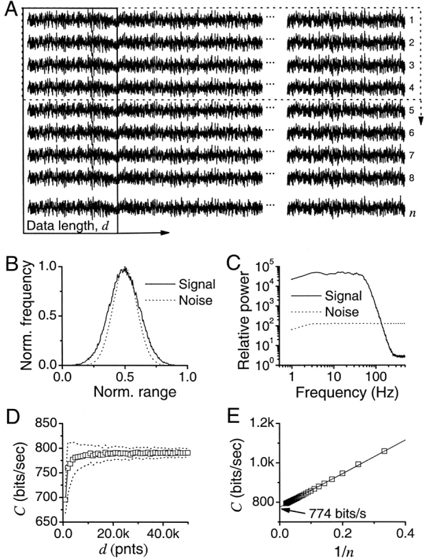
Calculation of information capacity, C. (A) Synthesized traces with Gaussian signal and Gaussian additive noise. Pass-band and stop-band for the signal are 70 and 120 Hz, respectively, whereas the noise is white. C (see Eq. 7) is estimated by using both different data lengths, d (indicated by the box with the arrow pointing right), and the number of trials, n (indicated by the dotted box with the arrow pointing down). (B) For long simulations with many repetitions, the signal and noise distributions are Gaussian. (C) Corresponding signal and noise power spectra. (D) C increases with the length of the data. Mean and SD shown. (E) Number of trials affects C; calculated from the data having 50,000 points. C is extrapolated by using the linear trend as .

In the case of Gaussian white noise stimulation and Gaussian additive noise, the signal is the mean response, and the noise is the difference from that mean. In our experiments we give n repetitions of an input of length, d. Fig. 6 B shows the distributions for the signal and the noise and Fig. 6 C the power spectra using a Fast Fourier Transform. To calculate the power spectra, the signal and noise traces are segmented using a Blackman-Harris four-term window with 50% overlap of segments (Bendat and Piersol, 1971; Harris, 1978). The data has 1 kHz resolution (t = 1 ms), so we set the size of the segments to 1,024 points. This fixes the minimum and maximum frequencies of the spectra to 0.977 and 512 Hz, respectively. The length of voltage responses dictates the number of samples of spectra: 1.024 s of data gives one signal and noise spectrum, whereas 10 s of data with overlapping segments gives 18 samples of spectra, each having a 512-point resolution. These are averaged in frequency domain to obtain smooth spectral estimates. The corresponding power spectra, S(f) and N(f), are then the real-valued (one-sided) autospectral density functions (Bendat and Piersol, 1971) and the signal-to-noise ratio, SNR(f), of the voltage responses is simply their ratio. SNR(f) is used to calculate the information capacity, C, given by the Shannon formula,

(7)

We now discuss the effect of the data length, d, and the number of repetitions, n.

Effect of Data Length on the Information Capacity Estimate

Fig. 6 D shows the dependence with the data length using n = 100 repetitions of a white noise stimulus. The data length in the graph varies from 1,000 to 50,000 points with the signal's pass-band and stop-band set to 70 and 120 Hz, respectively. Only after 10,000 points we observe convergence of the capacity values. To calculate the standard deviation, we repeat this calculation 1,000 times, shown in Fig. 6 D as a dotted line. The Shannon capacity converges to a value of 785 bits/s.

Effect of Repetitions

We use the values obtained from convergence at large lengths and we plot them in Fig. 6 E for different repetitions, n. Note a clear linear trend that extrapolates to a value of 773 bits/s. Note that large errors can take place if we do not use a large enough number of repetitions. Alternatively, a smaller number of repetitions could be used together with an extrapolation, such as the bias correction derived in van Hateren and Snippe (2001).

Details of the Triple Extrapolation Method

The triple extrapolation method has been described in the main text from Eq. 1 to 4. The purpose of this section is to show practical expressions for the entropies and a graphical tour of the calculations involved. We also show that for the mutual information the difference between the discretized mutual information converges to the continuous (integral) expression in the limit of small intervals

Eq. 2 follows from Eq. 1 simply rearranging terms and using that P _LS(l _i,s _i) = P _LS(l _i|s _i)P_S(s _i). We can separate the information into two terms, one for the total response and another for the noise as I_LS = H_S − H_N, with H_S the total entropy of the responses and H_N the entropy of the noise as and . Using these expressions for the signal and noise entropies, the expression for the information rate in Eq. 2 follows. As described in the main text, we discretize the photoreceptor signal in “words” of length T with T/t “letters.” Let P_S(s_i) be the probability of finding the i-th word. A naive estimate of the total entropy of the graded responses is given by:

(8)

This estimate depends on the size of the data, the length of the word, T, and the number of digitized voltage levels, v. The total entropy can be calculated as

(9)

and the total entropy rate as

(10)

The noise entropy rate is the average of the uncertainties of the graded responses to the different inputs. To calculate the noise we consider different trials of length T_trial. Let P _i(τ) be the probability of finding the i-th word at a time τ after the initiation of the trial. A naive estimate of the noise entropy is then obtained as

(11)

The noise entropy rate is then of the form:

(12)

and the information rate is R = R _S − R _N. As explained in the main text (see paragraph after Eq. 4 and Fig. 1 C), we use a concatenated triple extrapolation method to avoid the sampling catastrophe.

Independence of I on Bin Size with Bin Size Being Small

The dependence of the entropy on the bin-size, Δ, is given in Theorem 9.3.1 of Cover and Thomas (1991) as:

(13)

with S the integration limits for the variable x. The logarithmic divergences −log₂Δ present in the entropies cancel out in the transformation transfer as:

(14)

(15)

Graphical Tour to the Triple Extrapolation Method

First, we illustrate the calculation of the total entropy rate and then the noise entropy rate by using parameters that make simple graphs. For clarity, we start assuming that the method is just one extrapolation to infinite word lengths, fixing the data size and the number of voltage levels, v (Fig. 7) . After this we explain the steps of the triple extrapolation method (see Fig. 8).

Figure 7.

Total entropy and noise entropy rate of data digitized to four voltage levels. Calculation of the signal entropy rate R _S: (A) response and (B) its four-level digitization. (C) All possible two-letter words with four letters. (D) Frequency of the two-letter words in the word order given in (C). (E) Total entropy rate R _S extrapolated with a linear fit (, for T = 2, ▪). Calculation of R _N: (H) noisy responses (F) digitized to four voltage levels. The first and last two-letter words are highlighted in each trace. (G) Frequency of two-letter words at time τ = 551 ms. (H) Same as G for time τ = 559 ms. The noise entropy rate is given in E. (○) and (•). (G) Noise entropy rate R _N is extrapolated in the same way as for R _S.

First Step: Calculation of the Total Entropy Rate, R_S (Fig. 7, Left)

i. Digitization.

A single voltage response (Fig. 7 A) can be digitized into any number voltage levels, v, which defines the maximum number of different “letters” that make up the response. For illustrative purposes we use four voltage levels, v = 4 (Fig. 7 B).

ii. Segmentation into Letters and Words.

Four letters make 16 possible two-letter words (“11”, “12”, “13”,…”44”. v^T = 4², Fig. 7 C), 64 (4³) three-letter words and so on. Fig. 7 B shows the two-letter words in the response, here in a 50-ms window. Notice, that since the words do not overlap, a data-file with 1,000 time bins (or letter spaces, here t = 1 ms) contains 500 two-letter words.

iii. Calculation of the Probability Density P_S(s) for Different T.

Fig. 7 D shows the corresponding P_S(s) when T = 2, calculated from ten 1,000 point long responses. “33” is the most common two-letter word. Notice that words like “13” and “41” are not present in this data.

iv. Calculation of the Total Entropy.

The H _S ^T for each T was calculated as in Eq. 9.

v. Calculation of the Total Entropy Rate, R_S.

We divide H _S ^T by T and extrapolate to the infinity limit of T (Fig. 7 E). R_S is obtained by a linear extrapolation through seven points.

Second Step: Calculation of the Noise Entropy Rate, R_N (Fig. 7, Right)

i. Digitization.

Fig. 7 F shows ten 10-point long samples of voltage responses to the same repeated stimulus sequence that lasts 1,000 ms. The responses are digitized to four voltage levels (ν = 4; Fig. 7 I). The first and the last two-letter-words of the response samples are highlighted, occurring at the moments 551 and 559 ms, respectively.

ii. Calculation of the Probability Density P(τ) for Different T.

Having only 10 repetitions, both P(τ = 551) and P(τ = 559) for T = 2 are coarse (Fig. 7, G and H, respectively). Similarly, P(τ) for T = 2 is calculated for all the other 498 two-letter positions that occupy the remaining 996 data-points.

iii. Calculation of the Noise Entropy.

The H _N ^T for each T was calculated as in Eq. 11.

iv. Calculation of the Noise Entropy Rate R_N.

H _N ^T is divided by T and R_N (bits/s) is obtained by extrapolation to the infinite word length limit (Fig. 7 E).

Third Step: Calculation of the Information Transfer Rate

R = R_S − R_N for this data, digitized to four voltage levels, is 327 bits/s (Fig. 7 E).

For clarity, we have given these steps without making reference to the first two extrapolations. In the following we discuss details of the three extrapolations. The triple extrapolation method is computationally expensive, but gives an accurate estimate of information rate R for sufficiently large data-files. Fig. 8 illustrates the extrapolations for 1,000 repetitions of 1,000 points long segments of the synthetic data in Fig. 6.

Figure 8.

The triple extrapolation method. First extrapolation to infinite data size. (A) of the two-letter words (bottom) and of 10-letter words (top) of the responses for different voltage levels (v = 2–20) and fitted with quadratic Taylor series. and are obtained from extrapolations of and , respectively, for size→∞; [H _S ^T=2,2= ⋆; H _S ^T=2,20= Δ; H _S ^T=10,2= ★; H _S ^T=10,20= ▴]. Here, the probability of two-letter words is similar in all data fractions so size corrections in are minimal, whereas for 10-letter words size corrections have a bigger impact on H _S ^T=10,v. Second extrapolation to infinite voltage levels. (B) H _S ^T,v is shown for words of 2 and 10 letters, fitted here with both quadratic Taylor series (thick black lines) and exponentials (thin dotted lines). H _S ^T is obtained from the extrapolation of H _S ^T,v when ν→∞; H _S ^T=2 = open hexagon; H _S ^T=10 = closed hexagon, extrapolated from the Taylor fits. Third extrapolation. Entropy rates obtained from extrapolations to infinitely long words. (C) The total entropy rate, R _S (□), is obtained from a linear extrapolation of when T→∞. R _N (○) for the same data. Both R _S and R _N collapse to zero when the data is insufficient to provide an adequate extrapolation of H _S ^T and H _N ^T for long words and high voltage resolutions. The graph, however, shows enough linearly aligned points for accurate estimations of R _S, R _N, and R. (D) Effect of the number of voltage levels v used in the second extrapolation on R. The first point for the second extrapolation is the sixth voltage level. Taylor series of second order (▪) gives a good estimate when v = 11–25 for this data length. Exponential fits (○, using the second voltage level as the first point for the second extrapolation) compare worse with the capacity value. (E) Effect of data size on R. For >20 repetitions of 1,000 points long samples an accurate R (▪) is obtained. The length of the data sample should be at least 600 points long when repeated 1,000 times (□). Second extrapolation by Taylor series of second order with v ranges of 6–14 for H _S ^T and 6–16 for H _N ^T, respectively.

1. Infinite Data Size Extrapolation to Obtain H _S ^T,v and H _N ^T,v.

First, the data is digitized to different voltage levels, (here v = 2, 3…20, i.e., altogether 19 v levels). At each voltage level v, naive H _S ^T,v,size and H _N ^T,v,size are calculated for words of 1–20 letters (T = 1, 2…20; Eqs. 8 and 11, respectively) using 10 fractions of data (1/10, 2/10, 3/10…1). Hence, for one v this gives 200 and altogether 200 × 19 = 3,800 naive estimates for both H _S ^T,v,size and H _N ^T,v,size. Next, we search for trends in H _S ^T,v,size and H _N ^T,v,size for a given word length T at different data sizes. Simple trends emerge for both H _S ^T,v and H _N ^T,v and are extrapolated using quadratic Taylor series (Fig. 8 A shows (bottom) and (top) with the fits, for v = 2 and v = 20).

2. Infinitely Fine Voltage Resolution Extrapolation to Obtain H _S ^T and H _N ^T.

For each H _S ^T,v and H _N ^T,v, we fit the trend as v approaches infinity. Quadratic Taylor series provide a robust extrapolation of H _S ^T and H _N ^T over a large range of voltage levels (Fig. 8, B and D) and was used throughout this study (see Table I). For a small range of v (between 7 and 14 voltage levels) fitting H _S ^T,v by exponentials gives relatively similar values for H _S ^T (Fig. 8, B and D).

3. Infinitely Long Word Extrapolation to Obtain R_S and R_N.

H _S ^T and H _N ^T values are divided by T and the rates are extrapolated to the infinite word length limit (Fig. 8 C). For the exemplary data, this gives us a linear trend to obtain R_S and R_N by extrapolations. When using quadratic Taylor series for the first two extrapolations, R, the difference between R_S and R_N varies from 760 to 780 bits/s depending on the range of points taken for the final linear extrapolation (see also Fig. 8, D and E). This compares favorably with the corresponding information capacity estimate of 773 bits/s (Fig. 6).

Practicalities of Correcting Entropies by Size

If the data file is large enough that small fractions of it give accurate probability distributions for words of large T and v, the total entropy and noise entropy trends remain flat for lower T and v with increasing data size, and no size correction is required for H _S ^T,v and H _N ^T,v. For the given amount of synthetic WN data (as in Fig. 8), the entropies always rise with increasing data size and thus require the size correction. However, for many photoreceptor recordings we found the size correction negligible.

Minimum Data Size for Information Rate Estimation

Depending on the behavior of the data, 20 repetitions of 1,000 points long data file can be sufficient for the triple extrapolation method to provide a good R estimate (Fig. 8 E). On the other hand, the method provides an accurate R estimate for the given data files when they are at least 600 points long.

References

- Atick, J.J. 1992. Could information-theory provide an ecological theory of sensory processing? Network-Comp. Neural. 3:213–251. [DOI] [PubMed] [Google Scholar]
- Barlow, H. 1996. Intraneuronal information processing, directional selectivity and memory for spatio-temporal sequences. Network-Comp. Neural. 7:251–259. [DOI] [PubMed] [Google Scholar]
- Balasubramanian, V., D. Kimber, and M.J. Berry. 2001. Metabolically efficient information processing. Neural Comp. 13:799–815. [DOI] [PubMed] [Google Scholar]
- Balasubramanian, V., and M.J. Berry. 2002. A test of metabolically efficient coding in the retina. Network-Comp. Neural. 13:531–552. [PubMed] [Google Scholar]
- Bendat, J.S., and A.G. Piersol. 1971. Random Data: Analysis and Measurement Procedures. John Wiley & Sons, Inc., New York/London/Sydney/Toronto. 566 pp.
- Borst, A., and F.E. Theunissen. 1999. Information theory and neural coding. Nat. Neurosci. 2:947–957. [DOI] [PubMed] [Google Scholar]
- Buracas, G.T., A.M. Zador, M.R. DeWeese, and T.D. Albright. 1998. Efficient discrimination of temporal patterns by motion-sensitive neurons in primate visual cortex. Neuron. 20:959–969. [DOI] [PubMed] [Google Scholar]
- Burton, B.G. 2002. Long-term light adaptation in photoreceptors of the housefly, Musca domestica. J. Comp. Physiol. A. Neuroethol. Sens. Neural Behav. Physiol. 188:527–538. [DOI] [PubMed] [Google Scholar]
- Cover, T., and J. Thomas. 1991. Elements of Information Theory. John Wiley & Sons, Inc., New York 542 pp. [Google Scholar]
- de Polavieja, G.G. 2002. Errors drive the evolution of biological signaling to costly codes. J. Theor. Biol. 214:657–664. [DOI] [PubMed] [Google Scholar]
- French, A.S. 1980. Phototransduction in the fly compound eye exhibits temporal resonances and a pure time delay. Nature. 283:200–202. [DOI] [PubMed] [Google Scholar]
- French, A.S., M. Korenberg, M. Järvilehto, E. Kouvalainen, M. Juusola, and M. Weckström. 1993. The dynamic nonlinear behavior of fly photoreceptors evoked by a wide range of light intensities. Biophys. J. 65:832–839. [DOI] [PMC free article] [PubMed] [Google Scholar]
- Gabbiani, F., W. Metzner, R. Wessel, and C. Koch. 1996. From stimulus encoding to feature extraction in weakly electric fish. Nature. 384:564–567. [DOI] [PubMed] [Google Scholar]
- Harris, F.J. 1978. On the use of the windows for harmonic analysis with the discrete Fourier transform. P. IEEE. 66:51–84. [Google Scholar]
- Hevers, W., and R.C. Hardie. 1995. Serotonin modulates the voltage-dependence of delayed rectifier and shaker potassium channels in Drosophila photoreceptors. Neuron. 14:845–856. [DOI] [PubMed] [Google Scholar]
- Jackson, M.B., A. Konnerth, and G. Augustine. 1991. Action potential broadening and frequency-dependent facilitation of calcium signals in pituitary nerve terminals. Proc. Natl. Acad. Sci. USA. 88:380–384. [DOI] [PMC free article] [PubMed] [Google Scholar]
- Jansonius, N.M. 1990. Properties of the sodium-pump in the blowfly photoreceptor cell. J. Comp. Physiol. A. Neuroethol. Sens. Neural Behav. Physiol. 167:461–467. [Google Scholar]
- Juusola, M. 1993. Linear and non-linear contrast coding in light-adapted blowfly photoreceptors. J. Comp. Physiol. A. Neuroethol. Sens. Neural Behav. Physiol. 172:511–521. [Google Scholar]
- Juusola, M., E. Kouvalainen, M. Järvilehto, and M. Weckström. 1994. Contrast gain, signal-to-noise ratio and linearity in light-adapted blowfly photoreceptors. J. Gen. Physiol. 104:593–621. [DOI] [PMC free article] [PubMed] [Google Scholar]
- Juusola, M., A.S. French, R.O. Uusitalo, and M. Weckstrom. 1996. Information processing by graded-potential transmission through tonically active synapses. Trends Neurosci. 19:292–297. [DOI] [PubMed] [Google Scholar]
- Juusola, M., and A.S. French. 1997. The efficiency of sensory information coding by mechanoreceptor neurons. Neuron. 18:959–968. [DOI] [PubMed] [Google Scholar]
- Juusola, M., and R.C. Hardie. 2001. a. Light adaptation in Drosophila photoreceptors: I. response dynamics and signaling efficiency at 25°C. J. Gen. Physiol. 117:3–25. [DOI] [PMC free article] [PubMed] [Google Scholar]
- Juusola, M., and R.C. Hardie. 2001. b. Light adaptation in Drosophila photoreceptors: II. Rising temperature increases the bandwidth of reliable signaling. J. Gen. Physiol. 117:27–41. [DOI] [PMC free article] [PubMed] [Google Scholar]
- Kirschfeld, K. 1967. Die Projektion der optischen Umwelt auf das Raster der Rhabdomere im Komplexauge von Musca. Exp. Brain Res. 3:248–270. [DOI] [PubMed] [Google Scholar]
- Koch, C. 1999. Biophysics of Computation. Information Processing in Single Neurons. Oxford University Press, New York/Oxford. 562 pp.
- Laughlin, S.B. 1981. A simple coding procedure enhances a neuron's information capacity. Z. Naturforsch. [C]. 36:910–912. [PubMed] [Google Scholar]
- Laughlin, S.B., and R.C. Hardie. 1978. Common strategies for light adaptation in the peripheral visual systems of fly and dragonfly. J. Comp. Physiol. A. Neuroethol. Sens. Neural Behav. Physiol. 128:319–340. [Google Scholar]
- Laughlin, S.B., R.R.D. van Steveninck, and J.C. Anderson. 1998. The metabolic cost of neural information. Nat. Neurosci. 1:36–41. [DOI] [PubMed] [Google Scholar]
- Lewen, G.D., W. Bialek, and R.R.D. van Steveninck. 2001. Neural coding of naturalistic motion stimuli. Network-Comp. Neural. 12:317–329. [PubMed] [Google Scholar]
- Leutscher-Hazelhoff, J.T. 1975. Linear and non-linear performance of transducer and pupil in Calliphora retinula cells. J. Physiol. 246:333–350. [DOI] [PMC free article] [PubMed] [Google Scholar]
- Reinagel, P., and R.C. Reid. 2000. Temporal coding of visual information in the thalamus. J. Neurosci. 20:5392–5400. [DOI] [PMC free article] [PubMed] [Google Scholar]
- Rieke, F., D.A. Bodnar, and W. Bialek. 1995. Naturalistic stimuli increase the rate and efficiency of information transmission by primary auditory afferents. P. Roy. Soc. Lond. B. Biol. Sci. 262:259–265. [DOI] [PubMed] [Google Scholar]
- Sabatini, B.L., and W.G. Regehr. 1997. Control of neurotransmitter release by presynaptic waveform at the granule cell to Purkinje cell synapse. J. Neurosci. 17:3425–3435. [DOI] [PMC free article] [PubMed] [Google Scholar]
- Schönbaum, G., A.A. Chiba, and M. Gallagher. 1999. Neural encoding in orbitofrontal cortex and basolateral amygdala during olfactory discrimination learning. J. Neurosci. 19:1876–1884. [DOI] [PMC free article] [PubMed] [Google Scholar]
- Shannon, C.E. 1948. A mathematical theory of communication. Bell Syst. Tech. J. 27:379–423. [Google Scholar]
- Spekreijse, H., and L.H. van der Tweel. 1965. Linearization of evoked responses to sine wave modulated light by noise. Nature. 205:913. [Google Scholar]
- Stanley, G.B., F.F. Li, and Y. Dan. 1999. Reconstruction of natural scenes from ensemble responses in the lateral geniculate nucleus. J. Neurosci. 19:8036–8042. [DOI] [PMC free article] [PubMed] [Google Scholar]
- Strong, S.P., R.R. Koberle, R.R.D. van Steveninck, and W. Bialek. 1998. Entropy and information in neural spike trains. Phys. Rev. Lett. 80:197–200. [Google Scholar]
- Theunissen, F., J.C. Roddey, S. Stufflebeam, H. Clague, and J.P. Miller. 1996. Information theoretic analysis of dynamical encoding by four identified primary sensory interneurons in the cricket cercal system. J. Neurophysiol. 75:1345–1364. [DOI] [PubMed] [Google Scholar]
- Treves, A., S. Panzeri, E.T. Rolls, M. Booth, and E.A. Wakeman. 1999. Firing rate distributions and efficiency of information transmission of inferior temporal cortex neurons to natural visual stimuli. Neural Comp. 11:601–631. [DOI] [PubMed] [Google Scholar]
- van Hateren, J.H. 1986. Electrical coupling of neuro-ommatidial photoreceptor cells in the blowfly. J. Comp. Physiol. [A]. 158:795–811. [DOI] [PubMed] [Google Scholar]
- van Hateren, J.H. 1992. Theoretical predictions of spatiotemporal receptive-fields of fly lmcs, and experimental validation. J. Comp. Physiol. A. Neuroethol. Sens. Neural Behav. Physiol. 171:157–170. [Google Scholar]
- van Hateren, J.H. 1997. Processing of natural time series of intensities by the visual system of the blowfly. Vision Res. 37:3407–3416. [DOI] [PubMed] [Google Scholar]
- van Hateren, J.H., and C. Schilstra. 1999. Blowfly flight and optic flow II. Head movements during flight. J. Exp. Biol. 202:1491–1500. [DOI] [PubMed] [Google Scholar]
- van Hateren, J.H., and H.P. Snippe. 2001. Information theoretical evaluation of parametric models of gain control in blowfly photoreceptor cells. Vision Res. 41:1851–1865. [DOI] [PubMed] [Google Scholar]
- van Hateren, J.H., L. Ruttiger, H. Sun, and B.B. Lee. 2002. Processing of natural temporal stimuli by macaque retinal ganglion cells. J. Neurosci. 22:9945–9960. [DOI] [PMC free article] [PubMed] [Google Scholar]
- van Steveninck, R.R.D., and S.B. Laughlin. 1996. The rate of information transfer at graded-potential synapses. Nature. 379:642–645. [Google Scholar]
- van Steveninck, R.R.D., G.D. Lewen, S.P. Strong, R. Koberle, and W. Bialek. 1997. Reproducibility and variability in neural spike trains. Science. 275:1805–1808. [DOI] [PubMed] [Google Scholar]
- Wagner, H. 1986. Flight performance and visual control of flight of the free-flying housefly (Musca Domestica) II. Pursuit of targets. Philos. T. Roy. Soc. B. 312:553–579. [Google Scholar]
- Wheeler, D.B., A. Randall, and R.W. Tsien. 1996. Changes in action potential duration alter reliance of excitatory synaptic transmission of multiple types of Ca2+ channels in rat hippocampus. J. Neurosci. 16:2226–2237. [DOI] [PMC free article] [PubMed] [Google Scholar]
- Zettler, F. 1969. Die Abhängigkeit des ubertragungsverhaltens von frequenz und adaptationszustand gemessen am einzelnen lichtrezeptor von Calliphora erythrocephala Z. Vergl. Physiol. 64:432–449. [Google Scholar]