Ca²⁺ Sparks and Embers of Mammalian Muscle. Properties of the Sources

Abstract

Ca²⁺ sparks of membrane-permeabilized rat muscle cells were analyzed to derive properties of their sources. Most events identified in longitudinal confocal line scans looked like sparks, but 23% (1,000 out of 4,300) were followed by long-lasting embers. Some were preceded by embers, and 48 were “lone embers.” Average spatial width was ∼2 μm in the rat and 1.5 μm in frog events in analogous solutions. Amplitudes were 33% smaller and rise times 50% greater in the rat. Differences were highly significant. The greater spatial width was not a consequence of greater open time of the rat source, and was greatest at the shortest rise times, suggesting a wider Ca²⁺ source. In the rat, but not the frog, spark width was greater in scans transversal to the fiber axis. These features suggested that rat spark sources were elongated transversally. Ca²⁺ release was calculated in averages of sparks with long embers. Release current during the averaged ember started at 3 or 7 pA (depending on assumptions), whereas in lone embers it was 0.7 or 1.3 pA, which suggests that embers that trail sparks start with five open channels. Analysis of a spark with leading ember yielded a current ratio ranging from 37 to 160 in spark and ember, as if 37–160 channels opened in the spark. In simulations, 25–60 pA of Ca²⁺ current exiting a point source was required to reproduce frog sparks. 130 pA, exiting a cylindric source of 3 μm, qualitatively reproduced rat sparks. In conclusion, sparks of rat muscle require a greater current than frog sparks, exiting a source elongated transversally to the fiber axis, constituted by 35–260 channels. Not infrequently, a few of those remain open and produce the trailing ember.

INTRODUCTION

As an intracellular messenger, Ca²⁺ participates in a wide range of processes. In muscle, action potentials in the plasma membrane and transverse (T) tubules cause Ca²⁺ channels of the SR to open. The ensuing Ca²⁺ release initiates contraction (e.g., Cheung, 2002).

The study of this process (excitation-contraction coupling) was drastically altered by the realization that most, if not all, of Ca²⁺ release takes the form of Ca²⁺ sparks (Cheng et al., 1993; Tsugorka et al., 1995; Klein et al., 1996). The defining property of sparks is their abrupt termination, after an open time that in skeletal muscle varies narrowly around 5 ms. This brevity is reminiscent of the kinetic peak of Ca²⁺ release visible in the cell-averaged records, the similarity being a strong indication that the peak of Ca²⁺ release (which is a good representation of physiological response upon an action potential) may be just the result of superposition of synchronized sparks. Hence the relevance of Ca²⁺ sparks and their study.

Until very recently, it had been possible to study adult skeletal muscle sparks only in adult muscle of the frog. In mice and rats, the studies were largely restricted to myotubes in primary cultures. The adult produced few (Conklin et al., 1999) or no sparks, even in strong responses to voltage (Shirokova et al., 1998). The recent work of Kirsch et al. (2001) changed this situation, showing that sparks can be recorded in adult rodents in sufficient numbers to begin their biophysical study. This possibility is welcome, as it comes at a time when striking differences in the structures underlying Ca²⁺ signaling have been demonstrated between the two taxonomic classes, and when interesting transgenic mice are increasingly available.

Major differences in the molecular makeup of fast twitch muscles of frogs and mammals have long been known. First, the binding assays for dihydropyridines and ryanodine consistently yielded a lower dihydropyridine receptor (DHPR)/RyR for frogs, as if they had extra release channels. The early biochemical literature was reviewed by Shirokova et al. (1996). These authors took advantage of techniques developed by Delbono and Stefani (1993) and García and Schneider (1995) to carry out direct comparisons of Ca²⁺ release between frogs and mammals. A difference in the isoform complement of ryanodine receptors later became known, whereby the frog fast muscles contain RyR1 or α, and RyR3, or β, in approximately equal densities (for review see Sutko and Airey, 1996; Ogawa et al., 1999), whereas in most muscles of adult mammals the isoform 1 is found exclusively (Marks et al., 1989; Takeshima et al., 1989; Flucher et al., 1999). Finally, Felder and Franzini-Armstrong (2002) reported an association between the presence of RyR3 and extra channels, which in triadic cross sections appear as feet-like structures in a parajunctional position. These parajunctional channels are arranged in double or triple rows, but in glancing sections appear to constitute a lattice geometrically different than that of the junctional double row.

These disparate observations may reflect a fundamental structural difference in the supramolecular arrangement. The mammalian assemblage, made of a single release channel isoform in double row, connected with tetrads of voltage sensors in a well-known skipping pattern (Block et al., 1988), is complemented in the frog and other poikilotherms by a dual set of isoform 3 channels, located parajunctionally, and devoid of voltage sensors. It is reasonable to expect a functional correlate of these structural differences.

We undertook a systematic comparison of the morphology of Ca²⁺ sparks in mammalian and frog muscle, to derive information about Ca²⁺ release, and gating of release channels. An additional motivation was to elucidate the nature of embers, which were originally described as faint tails of voltage-elicited frog sparks (González et al., 2000b), but in the rat are much greater phenomena, leading or trailing a good fraction of spontaneous sparks and sometimes happening in isolation (Kirsch et al., 2001).

In this study we used fibers with a chemically permeabilized plasmalemma. This is because in our hands the mammalian response to voltage takes the form of a continuous, event-less release (Shirokova et al., 1998).

MATERIALS AND METHODS

Experiments were performed in segments of skeletal muscle fibers from the extensor digitorum longus of the rat (Rattus norvegicus, Sprague-Dawley) separated enzymatically, or singly dissected fiber segments from the semitendinosus muscle of Rana pipiens. 3-mo-old male rats were killed by CO₂ inhalation. EDL muscles of both legs were separated to their branches and pinned to a Sylgard chamber, which was filled with a modified Krebs solution plus 2 mg/ml collagenase type I and 10% fetal bovine serum, with no Ca²⁺ or Mg²⁺ added, and incubated in an orbital bath at 37°C for 1 h. Digested muscles were washed in Krebs solution plus FBS. After 30 min, fiber segments of ∼1 cm were removed gently and fixed slightly stretched (2.2 to 2.5 μm per sarcomere) to the glass bottom of a 100 μl Lucite chamber. The chamber was mounted on the stage of an inverted microscope (Axiovert 100 TV; ZEISS) equipped for confocal scanning of laser-excited fluorescence (MRC 1000; Bio-Rad Laboratories).

Adult frogs were anesthetized in 15% ethanol, then killed by pithing. The fibers, dissected and mounted in the confocal stage as described by González et al., (2000a), were moderately stretched to sarcomere lengths of 2.5 to 3.2 μm.

Immediately before saponization the fibers were briefly exposed to a relaxing (high [K⁺]) solution. All fibers were permeabilized by immersion in a glutamate-based internal solution (same as in Table I , but with 2 mM nominal [Mg²⁺] for rat fibers or 1 mM nominal [Mg²⁺] for frogs) containing 0.002% saponin and 50 μM fluo-3. Saponization was performed while monitoring fluorescence in the confocal system, so that penetration of dye could be assessed and exposure to saponin minimized (Launikonis and Stephenson, 1997). This allowed the use of a concentration of saponin lower than in earlier work (González et al., 2000a,b). Usually after 3 min saponin was washed out and the working solution (Table I) introduced in the chamber.

TABLE I.

Composition of Internal Solutions

	K(Cs)-Glutamate	K2SO4	EGTA	Total Ca	[Ca2+]	Total Mg	[Mg2+]	Na2ATP	Na2PC
		mM	mM	mM	mM	mM	mM	mM	mM
Rat glutamate	124		0.96	0.187	100	7.61	1	5.31	10.62
	124		0.96	0.319	200	7.61	1	5.31	10.62
	120		0.92	0.169	100	10.04	2	5.12	10.23
	120		0.92	0.291	200	10.03	2	5.12	10.23
Rat sulfate		90.0	1.06	0.204	100	7.92	1	5.35	10.58
		90.0	1.06	0.350	200	7.91	1	5.35	10.58
		86.6	1.02	0.186	100	10.73	2	5.15	10.29
		86.6	1.02	0.320	200	10.70	2	5.15	10.29
Frog glutamate	90		0.9	0.155	100	4.14	0.3	4.55	9.09
Frog sulfate		74.5	1.1	0.205	100	4.69	0.3	5.02	10.04

“PC” is phosphocreatine. Mg²⁺ and Ca²⁺ were added as Cl⁻ salts. Figures for [Ca²⁺] and [Mg²⁺] are nominal. All others are actual, after titration to pH 7 and dilution to an osmolarity between 315 and 320 mOsm/l (rat) or between 260 and 265 mOsm/l (frog). Solutions also had 5 mM glucose, 8% dextran, 10 mM HEPES, and 100 μM fluo-4 (except experiments with identifiers nnnn00, which had fluo-3).

Solutions

Experiments were performed at 17°C. Rat fibers were studied in either of the solutions listed in Table I, a glutamate-based solution with K⁺ as the main cation (essentially formulated by Kirsch et al., 2001), or a newly formulated SO₄ ²-based solution, otherwise similar to the glutamate solution. The composition of Krebs, Ringer, and relaxing solutions used in the preparation stages was given by Shirokova et al. (1996).

The scanning microscope was in standard fluorescein configuration (Ríos et al., 1999) and used a 40×, 1.2 n.a. water immersion objective (ZEISS). Line scan images shown are of fluorescence of fluo-4 (or fluo-3, in those with identifiers nnnn00), determined at 2-ms intervals at 768 points of abscissa x _j along a line parallel to the fiber axis. The pixel interval x was 0.1428 μm. The total time elapsed during acquisition of one image was 1,024 ms. Illumination for fluorescence excitation (100-mW Ar laser, 488-nm line attenuated to 3% power) caused some bleaching, evaluated and corrected as follows. Fluorescence intensity, F(x,t), was first averaged over x, after excising areas of excess fluorescence, to yield a function Φ(t), which in turn was divided by its average and low-pass filtered at 20 Hz to yield φ(t). This function, reflecting the bleaching effect, typically decayed ∼2% per second. A bleaching-corrected version of fluorescence was calculated as F(x,t)/φ(t) (henceforth represented as F(x,t)). Such function was then normalized to the baseline intensity F ₀(x), derived as an average of F(x,t) in the nonspark regions of the line scan image. Unless specified, images are not filtered before analysis, although for presentation purposes a two-dimensional digital filter at 0.33 of the Nyquist frequency was used throughout.

Line scan images were not taken repeatedly at the same location, to avoid photodamage. Exceptionally, when rare long-lasting events were observed (e.g., Fig. 8), repeated images were obtained at the same line, at ∼3-s intervals.

Figure 8.

Lone embers. (A and B) Line scan images obtained in succession on the same scan line. Images were digitally filtered at 0.33 of the Nyquist frequency. The spatial inhomogeneity in resting fluorescence shows that there was no spatial shift between the successive images. (C and D) Images after normalization, with time course of fluorescence averaged over seven pixels (or 1.00 μm) at the center of the ember. Identifier: 120700a3,4.

Detection and Morphology of Sparks

The quantitative characterization of spark morphology was performed on events identified by an objective detection program (Cheng et al., 1999, modified as in González et al., 2000a). For the present studies a first detection pass was performed with a threshold for detection determined relative to a regional measure of noise, then all events of amplitude below an absolute limit (0.3) were discarded. This dual pass procedure substantially reduced the number of false detections associated with such low amplitude criterion, while allowing for a more complete detection of narrow and brief events. When events were averaged (for the purpose of calculating release flux) additional selection criteria were used, and stated in each case.

The detection program carries out automatic determination of spark parameters: amplitude (peak F/F ₀), spatial half-width (full width above half magnitude [FWHM]* measured in the line scan that reached peak F/F ₀), rise time (from 10% to full peak), and full duration at half magnitude (both measured on the average of three central pixels). While parameters were measured on unfiltered images, the peak location of the spark, used for centering events in the construction of averages, was determined after two passes of 3-point smoothing. Because of the greater complexity of local events in the mammal, parametrizing their morphology required the definition of three additional measures: duration, which is the time span at the center of mass of the suprathreshold footprint, time to peak, the interval between the beginning of the suprathreshold portion and the peak, and average ember amplitude, only determined in cases when a steady ember was present.

The definitions above applied to the automatic quantification of individual events. When parameter values were determined on averaged events or on simulated events, the spatial width FWHM was calculated as 2(2ln2)^1/2 (or 2.3548) × σ determined on a shifted Gaussian function fitted to the spatial profile of the averaged spark or simulation, usually at the time of peak fluorescence. The fit also provided an amplitude, A.

(1)

Release Flux

Release flux was calculated as described by Ríos et al. (1999), on averages of the events located automatically. Because fluorescence images are obtained in scans along a line, the fluorescence information available is assumed to apply equally to all directions in space (i.e., sparks are assumed to be centered on the scanned line, and symmetric). Using this assumption, plus a specific scheme for dye reactivity and diffusion, the fluorescence of a spark and its surrounding space-time region is first processed to derive free [Ca²⁺] as a function of space and time. Then release flux is computed as the sum of binding fluxes to the known ligands (in turn calculated from diffusion-reaction equations). In the same way as earlier whole-cell methods (Baylor et al., 1983), this calculation assumes values for a set of parameters, which are listed in Table II and are used without changes for frog or rat, merely adjusting for changes in the concentrations of the relevant buffers (glutamate, fluo-x, EGTA) and for [Mg²⁺] or [Ca²⁺] if necessary. Two sets of parameter values, or “Models,” were used in parallel and are listed in the table. The first set, termed Model 1, consists of “consensus” values used by Ríos et al. (1999), with the addition of explicit binding and diffusion of glutamate, a poor buffer. The second set, Model 2, differed by the assumption of a threefold greater value for the diffusion coefficient of the dye and its Ca²⁺ complex. Volume integration of release flux density (with units of concentration over time) yielded a flux rate (quantity per unit time) that was converted to Ca²⁺ current.

TABLE II.

Values of Parameters Used by the Release Flux Algorithm and Simulations

Parameter/model	1	2	3	4
Fluo-3:Ca ON rate, 107 M−1s−1	3.2	3.2	3.2	3.2
Fluo-3:Ca OFF rate, s−1	33	33	33	33
EGTA:Ca ON rate, 107 M−1s−1	0.2	0.2	0.2	0.2
EGTA:Ca OFF rate, s−1	2	2	2	2
Trop:Ca ON-rate, 107 M−1s−1	0.57	0.57	0.57	0.57
Trop:Ca OFF-rate, s−1	11.4	11.4	11.4	11.4
ATP:Ca ON-rate, 107 M−1s−1	15	15	15	15
ATP:Ca OFF-rate, 104 s−1	3	3	3	3
ATP:Mg ON-rate, 107 M−1s−1	0.195	0.195	0.195	0.195
ATP:Mg OFF-rate, s−1	195	195	195	195
Glut:Ca ON rate, 107 M−1s−1	25	25	25	25
Glut:Ca OFF rate, 104 s−1	2,500	2,500	2,500	2,500
Parv:Ca ON-rate, 107 M−1s−1	12.5	12.5	12.5	12.5
Parv:Ca OFF-rate, s−1	0.5	0.5	0.5	0.5
Parv:Mg ON-rate, 107 M−1s−1	0.003	0.003	0.003	0.003
Parv:Mg OFF-rate, s−1	3	3	3	3
Maximum pump rate, mM s−1	9.8	9.8	9.8	9.8
[Troponin], mM	0.24	0.24	0	0.24
[Parvalbumin], mM	1	1	0	1
[Pump sites], mM	0.24	0.24	0	0.24
[EGTA], mM	1	1	1	1
[ATP], mM	5	5	5	5
DCa, 10−7 cm2s−1	35	35	35	52.5
Dfluo, 10−7 cm2s−1	2	6	2	3
DATP, 10−7 cm2s−1	14	14	14	21
Dglut, 10−7 cm2s−1	18	18	18	27
Dparv, 10−7 cm2s−1	0.16	0.16	0.16	0.24
DEGTA, 10−7 cm2s−1	0.36	0.36	0.36	0.54

Parv, parvalbumin. Trop, troponin. Glut, glutamate. [Ca²⁺] was 0.1 μM. [Mg²⁺] was 1 or 0.3, depending on the experiment.

Noteworthy in the current procedure is the adoption of a wider “workspace” of 65 pixels or 9.28 μm for the numerical computations. This yielded noticeably smoother results, probably because the boundary conditions apply better to the wider workspace.

Simulation of Sparks

Ca²⁺ sparks were simulated as the result of release from a source of known current and geometry, impinging on a homogeneous medium with the main Ca²⁺ binding and transport sites of the cytosol, as described by Ríos et al. (1999). In addition to a subresolution source, other simulations assumed a source greater than the resolution of the microscope. In those cases the source was cylindric, of subresolution radius, and a length of 3 μm (see illustration in Fig. 11). Reaction-diffusion equations describing the movements of Ca²⁺ and Ca²⁺-bound and Ca²⁺-free fluo-x in the presence of an isotropic myoplasm containing endogenous buffers were solved to calculate the concentration of Ca²⁺-bound dye, hence the fluorescence. The assumed release current was deposited uniformly into the source. Reaction-diffusion equations were solved numerically by PDEASE (Macsyma, Inc.) in a spheric volume of radius 4.3 μm. Control simulations in a larger volume gave results differing by <0.05 F ₀. The calculated fluorescence was a function of time and three spatial coordinates. Because the properties of the medium were isotropic, the spatial shape of the fluorescence was spherically symmetric when the source was a sphere, and axially symmetric when the source was a cylinder. A separate procedure, implemented in Fortran, was then used to “scan” the simulated fluorescence event. Such a scan could be at any spatial shift (in three directions) and form any angle with the axis of the cylindric source. The orientation was determined with two angles, θ and N, in perpendicular planes. The geometry of scanning is illustrated in Fig. 11. The simulation of scanning included blurring according to the experimentally determined point-spread function (PSF) of the imaging system (Ríos et al., 1999), idealized as a 3-D Gaussian function, with FWHM of 0.45 μm in the x-y plane and 1.44 μm in the z direction. For comparison of morphology parameters, random noise uniformly distributed in a range of 0.05 units of resting fluorescence was added to all simulated line scan images (rms = 0.014). For comparison with experimental averages, simulation averages were computed of line scans calculated using angles θ and ∅ that varied in a range consistent with the scanning orientation (additional description in discussion and Fig. 12).

Figure 11.

Simulated spark and scanning geometry. The diagram illustrates the network of transverse tubules (TT) and adjacent SR cisternae wrapping around myofibrils (M). A hypothetical source, i.e., release channels within the thick segment in red, is active. A spark (fluorescence, function of time and three space coordinates) was simulated assuming a 3-μm long source of 100 pA. Shown is the spatial picture after 2 ms. The corresponding scan image (examples in the following figure) is formed by line scans, calculated from this spark and the point spread function of the microscope at successive points in time. Intensity in the line scan depends on the position and angles of the source relative to the scanning line (in blue). In the diagram, x represents the scanning axis, y a perpendicular in the focal plane, and z the optical axis of the microscope. Three offsets (along x, y, and z), all of which are zero in the illustration, define the position of the spark. Two angles define its orientation: θ, between the spark axis and the z axis (∼45° in the figure), and φ, between the x-y projection of the spark axis and the x axis (zero in this figure).

Figure 12.

Sparks of brief rise time and their simulations. (A–C) Average of line scans of all sparks with rise time between 1.51 and 2.5 ms and amplitude greater than 1. (A) Longitudinally scanned rat sparks. (B) Transversally scanned rat sparks. (C) Frog, both directions. Color scale is chosen for visibility. (D) Temporal dependence of the averaged fluorescence at the spatial center of the sparks. Time constants of a single exponential decay fitted to the records: frog, 7.89 ms (in blue, from an average of 208 events); rat, longitudinal scans, 8.34 ms (in green, 49 events); transversal, 9.03 ms (in red, 21 events). (E) Spatial profile of averages at the time of peak fluorescence, color coded as in D. FWHM: frog, 1.26 μm; rat, longitudinal, 2.03 μm; transversal, 2.53 μm. (F–H) Line scan images of simulated sparks, using parameter values of Model 2. (F and G) 3 μm cylindric source of 150 pA, open for 2 ms. (F) Longitudinal scanning, simulated as an average of five scans, with offsets of zero in all directions, orientation angle φ = 80 degrees and θ = 5, 25, 45, 65, or 85 degrees. (G) Transversal scanning, an average of five scans at zero offset, with φ = 10 degrees and the same five values of θ. (H) Single line scan, with zero offset, of a spark simulated with a spheric 0.15 μm radius source of 50 pA, open for 2 ms. Random noise uniformly distributed within a 0.05 range of relative fluorescence units was added to all simulated images.

Parameter Values in Simulations

To explore the range of possible spark morphology, the simulations used a wide range of parameter values and two different assumptions for the dye–Ca²⁺ interaction. The sets of values used, termed “Models,” are given in Table II. Model 1 used the consensus values of Ríos et al. (1999). Model 2 used the same values and a much greater diffusion coefficient for the dye and its Ca²⁺ complex. Models 1 and 2 were also applied in all calculations of release flux (as described above). In Model 3, the concentration of all intrinsic binding sites (troponin, sites on the SR pump, parvalbumin) were set to 0. In Model 4, diffusion coefficients of all mobile species (dye, EGTA, ATP, glutamate, parvalbumin, as well as Ca²⁺ and its complexes) were increased by 50%. An additional set of simulations, with results available as additional material on line, used a more realistic scheme for the reactions of the dye (Baylor et al., 2002), whereby it could have ternary interactions with fixed sites in the cell and Ca²⁺.

Statistics

Significance of differences of averages was evaluated by the two-tailed Student's t test. The significance of the improvement of fit by a two exponential function compared with a single exponential was evaluated with the likelihood ratio statistic, LRS = (ssr₁ − ssr₂)/σ² (Hoel, 1971; Hui and Chandler, 1990), in which ssr₁ and ssr₂ are the sums of squares of the residuals, respectively, for the single and two-exponential fits and σ² is the variance of the record. LRS has a χ² distribution with two degrees of freedom. If the statistic exceeds 6.0 the improvement in fit provided by the two-exponential function is significant to better than 5%. σ² was estimated by ssr₁/(N − 5), which, being probably an overestimate, yields an underestimate of the statistic, hence underestimates the merit of the two-exponential approximation.

When averages of small samples not normally distributed were compared (as in Table VI), the significance of differences was compared also by the Mann-Whitney rank-sum test. In all cases the significance levels established by parametric and nonparametric tests were qualitatively consistent.

Online Supplemental Material

The additional material (available at http://www.jgp.org/cgi/content/full/jgp.200308796/DC1) expands simulations to include results with a ternary scheme of dye reactions taken from Hollingworth et al. (1999).

RESULTS

In this section, the morphologic parameters of local events in the rat are compared with those of the frog, and it is demonstrated that rat Ca²⁺ sparks are anisotropic, elongated within a plane parallel to the Z disk. Then a class of events, those exhibiting a prolonged ember, are described, averaged, and processed to evaluate the underlying Ca²⁺ flux. Finally, isolated or lone embers are analyzed in the same way.

Morphology of Local Ca²⁺ Events in the Rat

As first noted by Kirsch et al. (2001), local events in rat EDL muscle are characteristically polymorphic. This is illustrated in Fig. 1 , a composite of four different line scans of fluorescence, from two cells permeabilized by exposure to a relaxing solution with saponin, then immersed in a “rat glutamate” internal solution (Table I). Fluorescence is shown normalized to the spatially resolved, time-averaged fluorescence in the non active portions of the image. As described by Kirsch et al. (2001), events could be typical sparks (first trace from the top), sparkless “embers” (second trace), better illustrated in Fig. 8, or consist of spark-like peaks followed (third and fifth) or preceded (fourth) by embers of variable amplitude and width. This variable morphology is in contrast to the stereotypical nature of the events obtained in frog cells. For illustration of differences, Fig. 2 presents a line scan image from a frog muscle fiber, prepared in a similar way and immersed in the frog solution homologous to rat glutamate (Table I).

Figure 1.

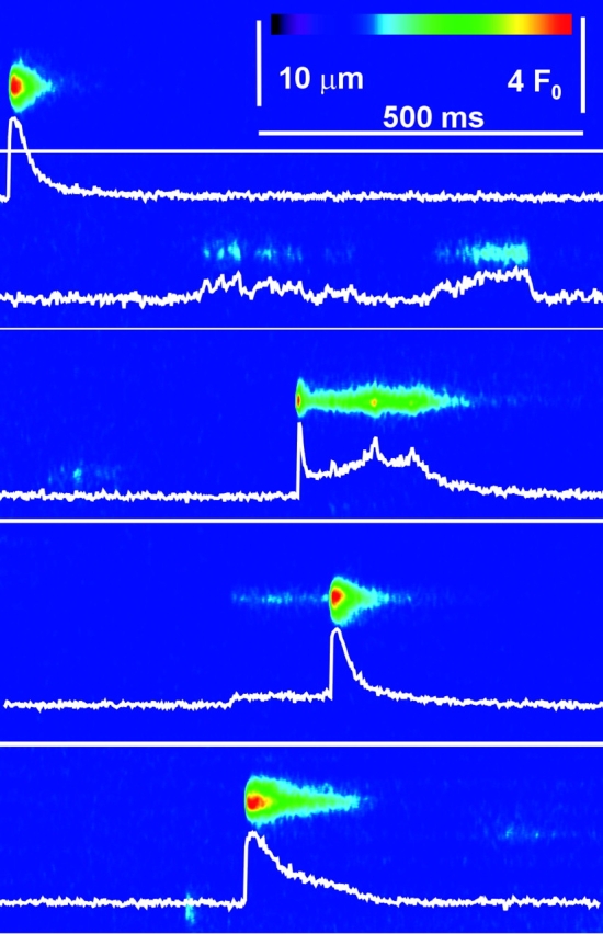
Sparks and embers in rat muscle. Collage of four line scan images of fluorescence in cells immersed in glutamate solution. Images were first corrected for bleaching (materials and methods). Corrected images were analyzed for initial location of sparks and a resting fluorescence F ₀(x) was calculated as the temporal average with spark regions excluded. The original images were normalized to F ₀(x) and digitally filtered in both dimensions at 0.33 of the Nyquist frequency. Cell and image identifiers, down from the top: 120700b11, 040401a4, 120700b69, 120700b62.

Figure 2.

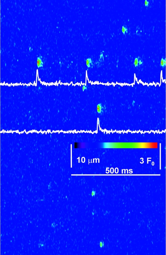
Sparks in frog muscle. Single line scan image from a frog cell in glutamate solution, normalized and filtered as described in Fig. 1. Identifier 102201c321.

Parameters were evaluated for ∼3,200 events in glutamate solution, automatically identified in 15 experiments. The frequency of events was variable between experiments and within the same experiment, tending to peak ∼20 min after membrane permeabilization, then decaying slowly over tens of minutes. The average frequency was 0.070 s⁻¹ per sarcomere. The mean values per experiment of parameters in all events, except those that were classified as “lone embers,” are listed in Table III .

TABLE III.

Morphology of Rat Events in Glutamate Solution

	Amplitude	FWHM	Duration	T to peak	Rise time	FDHM	N
		μm	ms	ms	ms	ms
071601b	0.57	2.07	43.02	12.65	8.85	14.00	51
071601a	0.54	2.03	39.94	14.49	8.02	12.18	391
062601a	0.59	1.92	43.87	13.82	7.57	11.69	175
062601b	0.62	2.07	37.89	13.18	7.28	10.43	318
061801a	0.51	2.00	45.49	13.37	8.00	12.84	617
061401b	0.65	1.95	43.22	16.20	6.44	9.45	430
061401a	0.60	1.87	41.44	15.19	6.86	10.20	261
052901a	0.46	2.51	49.75	13.97	9.09	16.29	55
052301c	0.43	2.21	38.68	13.55	9.14	14.77	38
052301b	0.51	2.33	43.31	12.66	8.56	15.24	122
052301a	0.50	2.00	45.23	13.27	7.95	12.64	47
040401a	0.82	1.97	75.24	27.50	5.87	48.69	132
120700a	0.69	1.84	62.73	28.85	6.94	42.28	151
120700b	0.75	1.99	64.20	24.74	7.40	11.90	174
120700c	0.59	1.86	56.06	22.87	6.65	9.67	254
Averages	0.59	2.04	48.67	17.09	7.64	16.82	3216
SEM	0.03	0.05	2.83	1.49	0.26	3.07

Parameters are defined in materials and methods. N is number of events detected automatically in all images of the same experiment, with criteria detailed in materials and methods. The averages and SEM in the last rows were calculated from equally weighted averages in individual experiments.

Comparison with Events in Frog Muscle

Because the internal solution was formulated with K⁺ as the main cation, while previous work with frog muscle used largely Cs⁺, we performed experiments with frog semitendinosus muscle in a comparable “frog K⁺ glutamate” or a “Cs⁺ glutamate” solution (Table I). The events recorded under such conditions were brief and stereotyped, similar to those in published works using Cs⁺-based internal solutions (e.g., González et al., 2000a,b). There were essentially no events with embers and none with more complex shapes.

A total of 1,890 events were collected in six frog cells, in either Cs⁺ or K⁺ glutamate. The average values of the parameters, listed in Table IV , were not significantly different in the two solutions. The average frequency of events (0.211 s⁻¹ per sarcomere) was similar in both solutions.

TABLE IV.

Morphology of Frog Events in Glutamate Solution

	Cation	Amplitude	FWHM	Duration	T to peak	Rise time	FDHM	N
			μm	ms	ms	ms	ms
101901a	K	1.01	1.47	41.13	11.94	4.93	16.44	1117
102201a	K	0.73	1.79	35.17	8.68	4.58	7.97	111
102201c	K	1.01	1.61	35.12	7.78	4.99	8.88	324
Average	K	0.92	1.63	37.14	9.47	4.83	11.10	1552
SEM		0.09	0.09	2.00	1.22	0.41	1.31
100901b	Cs	0.67	1.44	41.89	11.09	5.87	10.76	95
102901a	Cs	0.99	1.52	66.97	12.97	7.40	12.90	165
103001a	Cs	0.89	1.31	55.74	16.00	5.51	8.92	78
Average	Cs	0.85	1.43	54.87	13.36	6.26	10.86	338
SEM		0.10	0.06	7.25	1.22	0.41	1.31
Average	All	0.88	1.53	46.01	11.41	5.55	10.98	1890
SEM		0.06	0.07	5.20	1.22	0.41	1.31

“Cation” identifies the internal solution (either Cs⁺ or K⁺ glutamate, Table I). Averages and SEM for each cation were calculated from equally weighted averages in the experiments listed in each case. Averages and SEM in the last two rows were calculated from equally weighted averages in every individual experiment.

There were substantial differences between rat and frog parameters. The amplitude of the rat events was smaller by 33%. The rat events had substantially greater spatial width (2.04 μm) and a rise time ∼2 ms longer. In spite of these differences, sparks and embers were in most cases clearly identifiable, and in a first approximation it can be concluded with Kirsch et al. (2001) that most mammalian events consist of sparks, which may be riding on embers of varied properties.

Further illustration and analysis of the differences is in Figs. 3–5 . The histogram of spatial widths has a nearly monotonous decaying distribution for frogs, contrasting with a well-defined modal distribution, with a mode near 2 μm, for rats. The distribution of event durations in the frog (Fig. 3 B) could be fitted by a decaying exponential. The distribution of durations in the rat was better fitted as a sum of two exponentials. The improvement of the fit provided by the two-exponential function was highly significant (LRS = 12.72). The long-lasting component, of time constant 28 ms, comprises ∼83% of the sample mass and predicts that ∼0.5% of the population will have durations longer than 150 ms. Indeed, 49 events of durations in that range were identified. A study of events with long embers is presented below.

Figure 3.

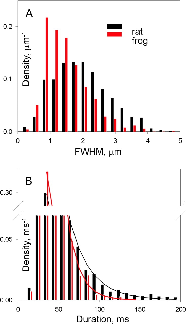
The distribution of spatial width and duration in rats and frogs. The rat histograms included all events listed in Table III (glutamate solution) and in Table IV (sulfate). The frog histograms included all events in Table V. The decaying portion of the frog duration histogram (B) was well fitted by a single exponential decay of τ = 13.5 ms. The rat duration histogram was fit better as the sum of two exponentials with τ₁ = 6.97 (factor a ₁ = 0.107) and τ₂ = 27.6 ms (a ₂ = 0.189).

Figure 5.

Averaged sparks in two orientations of scanning. (A–C) Average of line scans of all sparks with rise time between 4.01 and 6 ms and amplitude greater than 1. (A) Longitudinally scanned rat sparks. (B) Transversally scanned rat sparks. (C) Frog, all directions. Color scale is chosen for visibility. (D) Spatial profile of averages at the time of peak fluorescence. Frog data, in blue, from an average of 167 events (FWHM = 1.62 μm). Longitudinal rat scans, in green, 74 events (2.19 μm). Transversal rat scans, in red, 11 events (2.64 μm). (E and F) Spatial profiles at peak (continuous line) or 4 ms later (dashed), for average of rat longitudinal (green, E) or transversal scans (F); note crossing of curves in green. (G) Temporal dependence of the averaged fluorescence at the spatial center of the sparks, color coded as in D. Time constants of a single exponential decay fitted to the records: frog, 10.42 ms; rat, longitudinal, 14.29 ms; transversal, 12.66 ms.

Sulfate Increased Spark Frequency

While a large number of events could be collected in the rat, it was at the cost of examining thousands of images, given the low frequency of events. Additionally, there were many cells that did not produce events at a useful rate in either glutamate solution, or produced events transiently, and then stopped for no discernable reason. Serendipitously, it was found that a solution with SO₄ ²⁻ substituted for glutamate as the main anion (Table I) caused a slight increase in event frequency (to 0.08 s⁻ per sarcomere). More importantly, it stabilized frequency for any given cell, and reduced its variations among different cells. The average properties of events in SO₄ ²⁻ solution are listed in Table V . In spite of the differences in frequency and stability, no substantial differences were found between average values in SO₄ ²⁻ and glutamate solutions. Work in progress by Csernoch et al. (2003) indicates that, by contrast, SO₄ ²⁻ radically changes spark parameters in the frog.

TABLE V.

Morphology of Rat Events in Sulfate Solution

	[Ca2+]	Amplitude	FWHM	Duration	T to peak	Rise time	FDHM	N
	nM		μm	ms	ms	ms	ms
080701a	100	0.70	2.03	72.51	17.15	9.02	18.29	78
080701b	100	0.67	1.99	50.02	14.85	7.72	12.93	306
011002a	100	0.68	1.86	51.71	17.47	8.23	12.47	279
011602a	100	0.66	1.92	58.96	20.46	7.23	12.47	96
Averages	100	0.68	1.95	58.30	17.48	8.05	14.04	759
SEM		0.01	0.04	5.12	1.15	0.38	1.42
082401a	200	0.82	1.70	54.81	15.20	6.72	11.84	123
082801a	200	0.70	1.76	66.98	24.40	5.97	10.03	84
082801b	200	0.60	1.96	53.95	14.46	8.94	14.25	114
Averages	200	0.71	1.81	58.58	18.02	7.21	12.04	321
SEM		0.06	0.08	4.21	3.20	0.89	1.22
Averages	All	0.69	1.89	58.42	17.71	7.69	13.18	1,080
SEM		0.02	0.05	3.17	1.36	0.43	0.98

Morphology of rat events in sulfate solution. “[Ca²⁺]” is nominal in internal solution. Other columns have the same definitions as in previous tables. As shown, none of the average parameter values differs significantly in 100 and 200 nM [Ca²⁺]. Averages and SEM in the last two rows were calculated from equally weighted averages in all individual experiments.

Mammalian Muscle Ca²⁺ Sparks were Wider at All Rise Times

On average, mammalian sparks have a somewhat greater rise time (or source open time). To test whether their greater width is a consequence of the difference in rise time, the joint distribution of spatial width and rise time was examined. This is graphed for all events in longitudinal scans of rats or frogs in Fig. 4, A and B, as joint histograms interpolated by cubic convolution (González et al., 2000a). Both histograms show clear modes of rise times near 2 or 3 ms. They also show an evident difference in width at all rise times. A more quantitative comparison is made by calculating average spatial width in successive bins of rise time. The result, plotted in Fig. 4 C, shows major differences between the species. While in the rat the spatial width increases rapidly starting from the lowest rise times, in the frog the increase does not occur until 4 or 5 ms, and the average width stays lower than the rat value at all rise times. Relative differences in spatial width are most important at rise times from 2 to 5 ms, which is where the distribution modes are located. Because rat sparks are wider at all rise times, there must be reasons for the difference other than the increase in average rise time.

Figure 4.

Joint distributions of width and rise time. Joint histograms of rise time and spatial width were calculated for all frog (A) or rat events (B), in bins of 2 ms and 0.1428 μm. Frequencies were then interpolated by the technique of cubic convolution (Park and Schowengerdt, 1983; González et al., 2000a). (C) FWHM, averaged in contiguous bins of rise time, versus central rise time in each bin. Error bars represent one SEM in either direction. Frog values in blue.

An additional observation in rat fibers is the nearly identical relationship of spatial width and rise time exhibited by the sparks in glutamate and SO₄ ²⁻, in keeping with the assertion that in the rat the presence of SO₄ ²⁻ does not alter spark morphology.

Mammalian Muscle Sparks Are Elongated

The most striking difference between sparks in rat and frog fibers is the greater spatial width of the rat events, by 33% in the overall averages, but up to 80% greater in events with brief rise times (illustrated below). This indicates differences in mechanism. Indeed, while the spatial width of frog sparks in reference conditions (1.33–1.51 μm; Lacampagne et al., 1999; Klein et al., 1999; Ríos et al., 1999; González et al., 2000a) can be reproduced in model simulations that assume consensus buffer properties and subresolution sources (Chandler et al., 2003), it is difficult to explain wider events, unless radically different assumptions are made regarding the source geometry (see below). A wider spark requires in principle a Ca²⁺ flux increased in proportion to the third power of the increase in width, hence the underlying mechanisms will have to account for a much greater Ca²⁺ release current.

Alternatively, the cause of wider sparks could be structural differences leading to changes in diffusion coefficients or other parameters. As shown later, large differences of this sort were assumed in simulations, but could not explain the spark properties. Therefore, we hypothesized that the greater width in rat events reflects an extensive source, elongated in the direction of the T tubules. To test this hypothesis, events were collected under transversal scanning in two rat and two frog fibers.

The average parameter values are listed in Table VI . Event averages are compared in the table with similarly calculated averages for the longitudinally scanned events. In the rat case spatial width was ∼10% greater in the transversally scanned group, and no other significant differences were found. In the frog fibers the transversally scanned sparks were slightly narrower, but not significantly so. Because the distribution of widths was skewed (Fig. 3), the groups of spatial widths were also compared using a nonparametric test (the rank-sum statistic), which again resulted in significant difference between the rat but not the frog groups.

TABLE VI.

Comparison of Sparks under Two Directions of Scanning

	Species	Amplitude	FWHM	Duration	T to peak	Rise time	FDHM	N
			μm	ms	ms	ms	ms
080801a	rat	0.61	2.12	54.31	13.08	7.89	14.32	206
080801b	rat	0.81	2.36	50.51	14.87	7.05	12.37	35
Transversal averages	rat	0.64	2.15	53.76	13.34	7.77	14.03	241
SEM		0.02	0.05	2.74	0.86	0.42	0.53
Longitudinal averages	rat	0.62	1.97	49.18	16.77	7.49	14.14	4,296
SEM		0.00	0.01	0.49	0.27	0.09	0.44
102901a	frog	0.99	1.52	66.97	12.97	7.40	12.90	165
103001a	frog	0.89	1.31	55.74	16.00	5.51	8.92	78
Transversal averages	frog	0.96	1.46	63.37	13.94	6.79	11.62	243
SEM		0.04	0.05	1.75	0.90	0.36	0.45
Longitudinal averages	frog	0.97	1.52	39.59	10.85	4.97	14.05	1,647
SEM		0.01	0.02	0.31	0.25	0.10	1.05

Rows 2 and 3 list parameters of sparks in rat fibers scanned transversally to their axis. Averages are over individual events. “Longitudinal averages” are of individual events in all other rat experiments. Frog values are for fibers in glutamate solution, scanned transversally. “Longitudinal averages” are of individual events in all other frog experiments in glutamate solution.

Additional features of the difference between events are illustrated in Fig. 5. Based on the plot in Fig. 4 C, the difference in width between frog and rat sparks was most significant, in relative terms, for events of rise time near 5 ms. Averages of all events of rise times between 4 and 6 ms are compared in Fig. 5. (Only events of amplitude 1 or greater were included, to approximate an “in focus” condition, which will be assumed when comparing these averages with simulations.) There are major differences between the average of longitudinally scanned events in the rat (A) and the all-scans average in the frog (C). Fig. 5 E plots the spatial profiles of the averages at their peak. These profiles are approximately described by a Gaussian function (Eq. 1). The spatial half width of the averaged fluorescence calculated on the fitted Gaussian was 1.22 μm for the frog average and 2.19 μm for the average of longitudinally scanned rat events. Therefore, when events within this range of rise times are compared, the excess width is 80%, rather than the 33% difference obtained in comparisons of all events.

Also interesting is the effect of this restriction in rise times on the difference between sparks scanned in different directions. It results in a characteristic triangular shape for the transversal average (Fig. 5 B), contrasting with the “light bulb” appearance of the longitudinal average (Fig. 5 A). The different appearance reflects an earlier increase of spatial width in transversally scanned sparks. Thus, the profile of the average of transversally scanned sparks in this range of rise times, plotted in red in Fig. 5 D, had a FWHM of 2.64 μm, ∼20% greater than the longitudinal average of equal rise time. While width increased with rise time, the relative difference between the two orientations of scanning was greatest at the earliest rise time, and amounted to 34% at rise times near 2 ms. Averages within this range of rise times are illustrated in Fig. 12, and used for analysis in the discussion.

The longitudinal average (Fig. 5 A) owes its rounded appearance also to the fact that the spatial width appeared to rise after the time of peak amplitude (marked by the first arrow), so that the average became actually wider at times when its amplitude had started to decrease (a phenomenon termed “postpeak expansion,” second arrow). FWHM not only just grew after the fluorescence peak, but in longitudinally scanned images it did so more rapidly than before the peak. This led to a marked qualitative difference (key to the light bulb appearance in the longitudinal scans) illustrated in Fig. 5, E and F. The graphs show in solid line the spatial profiles at the time of the peak, and in dashed line the profiles 4 ms later, in Fig. 5 E for longitudinal scans (green) and in Fig. 5 F for transversal scans. For either direction, spatial width is seen to increase in the postpeak trace, but in the longitudinal scan, at distances of ∼2 μm, the fluorescence rises above the level reached at the peak of the spark (the plots cross). Such difference was observed between averages of events with rise time near 2, 5, or 7 ms, but was most marked at the shortest intervals. This fact, together with the observations that the difference in width with scan orientation was greatest at early times, and that the post-peak expansion was faster in sparks scanned longitudinally, can be explained if the source of current causing the spark is elongated. Put simply, when the scan of a long source is done perpendicularly to the source axis (that is, parallel to the fiber axis), the contribution to fluorescence from regions of the source away from the scan line will be detected later than those closer to focus. These spatiotemporal aspects are compared with properties of simulated sparks in the discussion.

The temporal profiles in Fig. 5 G show that the decay of rat sparks is somewhat slower. This may in part reflect the presence of embers in rat events, but the decay was slower even when long duration events were excluded. A slower decay could also be explained by a more extensive source, as shown later.

In summary, the examination of averages within restricted ranges of rise time confirms large differences in spatial width between species, strengthen the conclusion that rat sparks are elongated in the direction of the T tubules, and suggest that the elongation is due, at least in part, to the involvement of an elongated source. The rest of this section examines features related to gating of the spark sources.

Sparks with Long Embers

A remarkable feature of rat events, as already noted, was the presence of embers, which occur in manually peeled or intact cells as well (Kirsch et al., 2001). Based on a boundary of 50 ms for durations, Kirsch and colleagues estimated at 33% the fraction of sparks that had embers in chemically skinned rat cells. By the same criterion, 23% of the rat sparks in the present work had embers. In the majority of events with embers, these trailed the main spark (as in the third and fifth events graphed in Fig. 1). Others had leading embers, like the fourth event in Fig. 1. Such images pose the question of the magnitude and temporal properties of the Ca²⁺ release flux responsible for the ember.

Several studies have evaluated Ca²⁺ release underlying discrete events. We have done it with two complementary strategies (for review see Ríos and Brum, 2002). Both use deterministic equations of Ca²⁺ diffusion and binding to fixed and mobile cellular components, but they differ in their starting point. In the so-called “backward” calculation, the flux is derived from the measured fluorescence (Ríos et al., 1999). In the “forward” procedure, a flux (or current density, function of space and time) is assumed, and the resulting fluorescence event is calculated (Smith et al., 1998; Jiang et al., 1999; Ríos et al., 1999; Baylor et al., 2002; Soeller and Cannell, 2002). Then the assumptions for flux may be iterated seeking agreement between simulation and measured fluorescence (Soeller and Cannell, 2002). A somewhat different realization of a forward procedure is that of Uttenweiler et al. (2002), who calculate release flux as the product of a variable permeability and a [Ca²⁺] gradient, derived from explicit diffusion-reaction calculations in SR and cytosol.

We chose to apply the backward calculation algorithm to events with embers, rather than to the “standard” sparks for two reasons. First, the source of sparks is likely to be elongated, hence applying an algorithm that assumes spheric symmetry is likely to produce flawed results. In contrast, embers are due to lower release fluxes, originating in all likelihood at sources of subresolution dimensions, consistent with the assumptions of the algorithm. Moreover, the algorithm may also be applied to lone embers, providing a reasonable estimate of flux through a single channel.

Because the backward method involves repeated differentiation in space and time, it requires substantial averaging of the input signal to produce usable results. To evaluate the release flux underlying embers, the backward algorithm was applied to averages of events with long trailing embers. The selection criteria included duration greater than 160 ms, amplitude greater than 0.7 and time to peak <20 ms. Aspects of this selection and its consequences are illustrated in Fig. 6 A, depicting five hypothetical events. All but the first represent sparks with embers. The minimal duration criterion is represented by the double arrow. The selection process will reject the top two events and accept the next three. Therefore, the decaying (OFF) portion of their average will represent the average time course of their embers. If the duration criterion was changed to accept briefer events (so that the second example record would become acceptable), then the averaged OFF time course would not represent an average of embers, but the complex result of the termination of embers at different times. An additional aspect illustrated is that, as a consequence of “centering” the averaged records at their spark peak, the onset of the average will have kinetics that are slower and more graded than that of the individual events, because their beginnings will not be synchronized.

Figure 6.

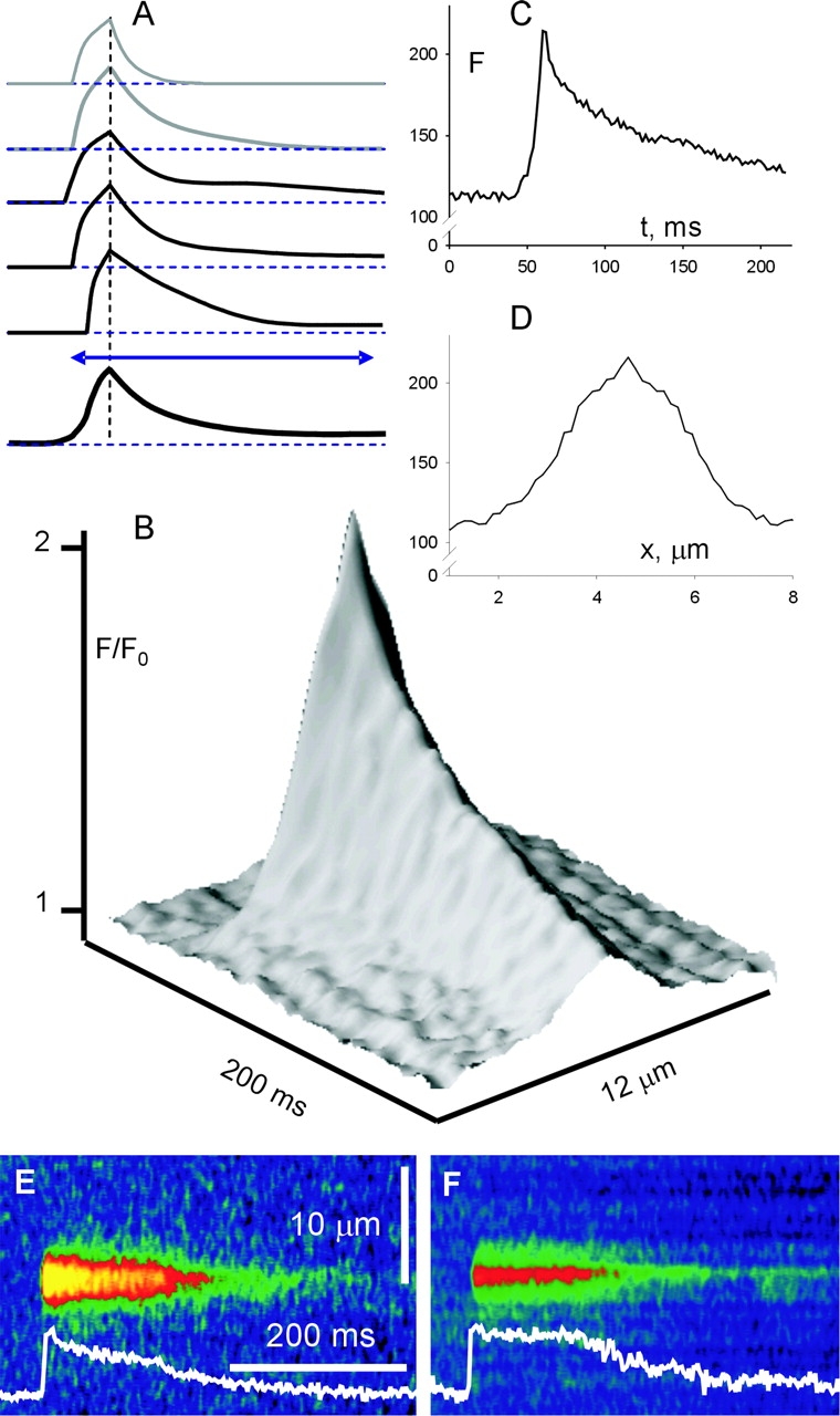
An average of sparks with long embers. (A) The selection criterion and its consequences. The selection process requires duration to be greater than the span represented by the double arrow. Of the five sparks represented above the double arrow, the first two, in gray, do not meet the criterion. The average of the other three is represented schematically in thick trace below the double arrow. (B) A surface shade plot of normalized fluorescence for the average of 49 events that met the criterion (duration > 160 ms, amplitude > 0.7). (C and D) Temporal and spatial profiles of fluorescence at the peak of the average. (E and F) Examples of sparks that met the selection criteria, but, unlike the average, show discontinuities in the slope of decay. The vertical bar represents 2 units of F₀ in E and 1 in F. Identifiers: E, 0814b100; F, 0824a27.

49 events satisfied the above conditions. The backward calculation algorithm was applied to their average (shown in Fig. 6 B). In prior applications this algorithm has been implemented with a “consensus” set of parameter values (Model 1 in Table II). In the present case a modified set (Model 2) was also used. This set was identical to the first one, except for a much greater diffusion coefficient of the dye (D_fluo) and its Ca²⁺ complex. In simulations, it performed best among many to reproduce the features of experimental sparks (discussion). The results are illustrated in Fig. 7 . In panel A are two representations of the flux density (in mM s⁻¹, Model 2), and in B is the release current, calculated with Model 1 (solid line) or 2.

Figure 7.

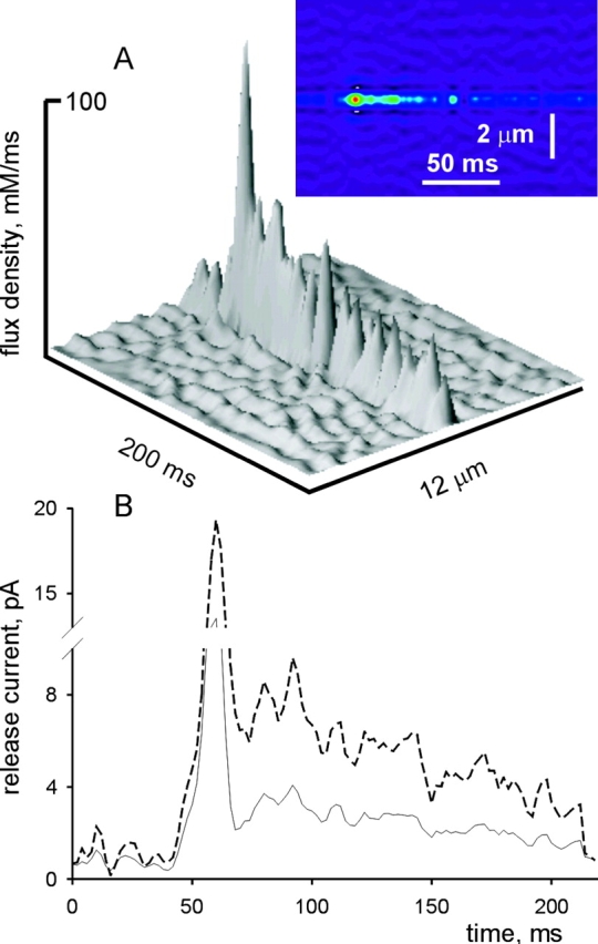
Ca²⁺ release flux in the average of events with long embers. (A) Two representations of release flux density derived from the average spark in Fig. 6 by the backward calculation algorithm, using Model 2 parameters. (B) Total Ca²⁺ release current, calculated from the flux density, under Model 1 (solid line) or 2. For model parameters see materials and methods.

Flux and current exhibit an early peak, at the time of rise of the spark, and then a lower level, corresponding to the ember. For reasons given before, the initial peak may not give a quantitative representation of the early flux. With either model, the flux decays slowly during the ember. The main consequence of the change of D_fluo was an increase of the current by a factor of ∼2. Changes in other diffusion parameters, which were less effective in modifying the calculated current, are explored with simulations in the discussion.

In conclusion, the Ca²⁺ release algorithm yields a slowly decaying Ca²⁺ release current during long-lasting trailing embers, with an initial value of 3 or 7 pA, depending on the assumptions.

Lone Embers

These are events that reach a steady amplitude and width after a monotonic onset, and in most cases last much longer than a spark. As an example, in Fig. 8, A and B , are unprocessed portions of scan images obtained successively at the same line. In C and D are the corresponding images after normalization. In this case the embers obviously originated at the same source. González et al. (2000b) and Shtifman et al. (2000) described similar events in frog muscle, produced by channel-opening ligands imperatoxin-A, ryanodine, and bastadin, and concluded that those embers were probably the consequence of drug-induced opening of single channels. It is under the same assumption that lone embers are studied here.

Properties of lone embers in glutamate and SO₄ ²⁻ are summarized in Table VII . Two far outliers, with amplitudes of 1.5 and 1.7, were not included in the averages. No difference was found between average parameters of these two groups.

TABLE VII.

Morphology of Lone Embers in Rat Muscle

		Amplitude	FWHM	N
			μm
Glutamate	Average	0.43	1.62	32
	SEM	0.036	0.097
Sulfate	Average	0.46	1.76	16
	SEM	0.044	0.157

All embers in the two internal solutions are included. When multiple embers originate at the same source in one image, as in Fig. 8, their average parameters are calculated and included as one individual value in the tabulation.

If lone embers indeed corresponded to single channels open for long intervals, it would follow that single channel openings result in steady release. Lone embers therefore suggest that Ca²⁺ release through a single channel does not cause depletion near the luminal channel mouth. A different view, leading to local depletion even with small fluxes, can be found in two recent papers (Sobie et al., 2002; Uttenweiler et al., 2002).

The presence of repeated embers from the same source, as in the illustration, made it possible to apply the “backward” release calculation. All close-to-open transitions leading to openings of 80 ms or longer, with fluorescence >0.25 were identified and collected. 18 transitions satisfied these criteria. They were averaged and centered at the spatial position of maximum fluorescence and at the time of threshold crossing. The average is shown in Fig. 9 . The release flux calculated with Model 2 is represented in Fig. 9 D and the current, with both models, in Fig. 9 E. The release current during the initial 80 ms of the ember average oscillates near 0.7 pA, with Model 1, or 1.3 pA with Model 2.

Figure 9.

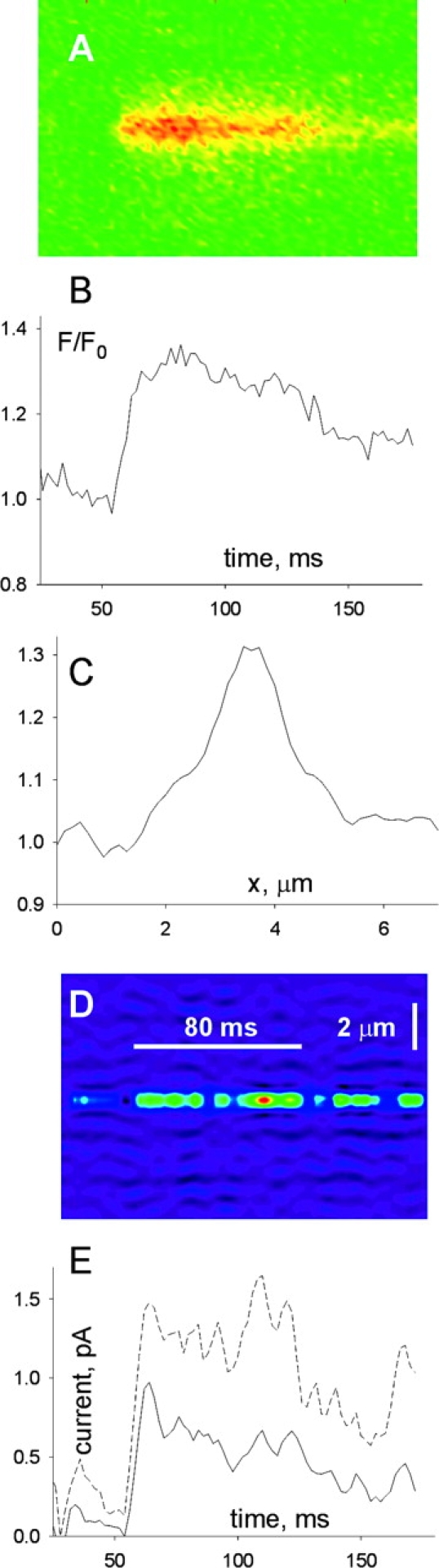
Flux in lone embers. (A) Average of opening transitions in 18 lone embers of amplitude >0.2 and duration >80 ms. The individual events were positioned in time so that their first point above threshold would coincide. (B) Temporal profile at the central pixel. (C) Spatial profile, obtained by averaging fluorescence during 50 ms, after the central fluorescence reached 80% of maximum. (D) Line scan representation of release flux density, calculated with the backward algorithm and Model 2. (E) Ca²⁺ release current, with Models 1 (solid line) or 2.

Given the values of Ca²⁺ release current at early times of the averaged trailing ember (Fig. 8 B), 3 pA (with Model 1) or 7 pA (Model 2), and the corresponding values in the averaged lone ember, it is concluded that early in the trailing ember 4 or 5 channels (7/1.3 or 3/0.7) remain open. If only a small number of channels remained open during a trailing ember, then it should be possible to observe step-wise closing, which should result in abrupt changes in the decay rate. Such was often the case, as illustrated by examples in the bottom panels of Fig. 6, as well as the bottom record in Fig. 1.

Events with Leading Embers

The fourth event plotted in Fig. 1 is an example of a spark preceded by an ember. The backward analysis of release is less practical in this case because it is not possible to construct a meaningful average that does not smear either the beginning of the ember or the spark. Instead, on this and other examples analyses were performed based on two linear approximations.

The first approximation was to compare the rates of rise of fluorescence in ember and spark, which are proportional, within limits, to the intensity of the source, provided that the source dimensions are below the limits of resolution of the imaging method (e.g., Smith et al., 1998; Shirokova et al., 1999a). Fig. 10 A includes a plot of fluorescence versus time (normalized, corrected for bleaching and averaged in the central 5 pixels of the signal). The initial transition, at the start of the leading ember, was fitted by an exponential, represented in thick trace. The rising phase of the spark was likewise fitted by an exponential, in thin trace. The maximum rates of rise (of the fitted exponentials) were 0.123 ms⁻¹ for the ember and 4.55 ms⁻¹ for the spark. Their ratio, 37, is therefore an estimate of the number of channels open in the spark, under the assumption that the leading ember corresponds to one fully open channel, and that the sources have dimensions below resolution.

Figure 10.

Rates of fluorescence change in a spark with leading ember. (A, dashed) Normalized fluorescence averaged over three central pixels of image in third panel of Fig. 1. Thick continuous line, single exponential fit to the overlapping region of the experimental curve. Parameters of fit: amplitude, 0.473; exponential rate constant, 0.261 ms⁻¹. Thin continuous line: single exponential fit to the overlapping points of the experimental curve. Parameters of fit: amplitude, 3.52; exponential rate constant, 1.30 ms⁻¹. (B) Continuous line: signal mass, calculated by volume integration of excess fluorescence over the baseline, assuming spheric symmetry. Dashed line: similar calculation, but spark was first smoothed by five points over time. An exponential fit, showed in continuous line, was used to evaluate the evolution of signal mass early in the leading ember. Parameters of fit: amplitude, 3.57 μm³; rate constant, 0.0376 ms⁻¹. Identifier: 120700b69.

This number is an underestimate. Indeed, when the source is made extensive (that is, of size greater than the limit of resolution of roughly 0.5 μm) then large currents may occur without a proportional increase in fluorescence (e.g., Smith et al., 1998). In these cases the spatial width of the signal increases, and a better estimator of release current can be found instead in the rate of production of signal mass (Sun et al., 1998; González et al., 2000a, Chandler et al., 2003). In the event of Fig. 1 the spatial width of the spark is much greater than that of the ember, hence the signal mass (proportional to the third power of spatial width under the assumption of spheric symmetry) will rise comparatively faster than the central fluorescence.

Signal mass was calculated by integrating the normalized fluorescence in the volume of the spark, assumed spherically symmetric. Under longitudinal scanning, the orientation of the T tubules is always perpendicular to the scan line. If the spark in question was elongated, rather than symmetric, then the calculation would underestimate signal mass.

The calculation is illustrated in Fig. 10 B. In continuous line is the signal mass calculated for each line (or time point) of the image, plotted versus time. From this plot, a maximum rate of production of mass, 21.45 μm³ ms⁻¹, was calculated as the average in the interval 504–508 ms. In dashed trace is the signal mass displayed in an expanded vertical scale, to show the early increase associated with the ember. (The signal mass in this case was calculated on a 5-point smoothed image to reduce noise.) The maximum rate of signal production was calculated as the initial slope of the fitted exponential (black, dashed). The result, 0.134 μm³ ms⁻¹, leads to a ratio of 21.45/0.134, or 160.

In conclusion, two analyses of this particular spark lead to estimates of 37 or 160 for the number of channels fully open at the time of maximum growth of the spark.

DISCUSSION

In the present work morphologic parameters were evaluated for Ca²⁺ sparks generated spontaneously in membrane-permeabilized cells of rat muscle. Morphology was evaluated for a vast database of events. The sole precedent for comparison is the work of Kirsch et al. (2001), on a smaller set of events in saponized mammalian muscle. The present results are in agreement as regards the polymorphism and proportion of different types of local events. However, there are differences: average amplitude was greater in the previous work, FWHM was smaller, while rise time and duration at half magnitude were much greater (∼48 ms in the previous work, vs. 7.6 and 16.8 ms here). These differences may stem in part from the fact that Kirsch and colleagues identified sparks by eye. Additionally, a definition of rise time that does not correct for the presence of a leading ember, will include the duration of the leading ember in this measure. In our case, the rise time started at the 10% rise above any leading ember.

The parameter values found in the present work make the differences with the events of frog muscle more obvious and striking.

Mammalian Muscle Events Were Wider and Longer-lasting

In the rat, the events were less frequent, and their occurrence less predictable than in equally prepared frog cells. Hence, an alternative solution, with SO₄ ²⁻ as main anion, which was found to increase frequency and reliability of event production, was also used.

Rat events were compared with events recorded in similarly prepared frog fibers in glutamate solution (which had measures consistent with previous works of Lacampagne et al., 1999; González et al., 2000a, in similar conditions). The most impressive differences were in amplitude, which was 50% greater in the frog, and spatial width, with a FWHM of ∼2 μm in longitudinal scans in the rat, compared with 1.5 μm in the frog. Other differences were a greater time to peak in the rat (indicative of the presence of leading embers), a greater duration (consequence of the presence of embers), and a somewhat greater rise time. The average parameter values in the rat were remarkably independent of the presence of sulfate or glutamate. (Work communicated preliminarily by Csernoch et al., 2003 finds instead that in the frog the substitution of SO₄ ²⁻ for glutamate causes substantial changes in spark morphology.)

Of the differences listed above, potentially most interesting is that of spatial width, for two reasons. It has been difficult to understand and reproduce the large spatial widths of experimental sparks. Simulations that assumed point sources with open time limited to 7 ms or less had spatial width close to 1 μm (Smith et al., 1998; Jiang et al., 1999; Ríos et al., 1999; Baylor et al., 2002). More recent work, using large currents, simulated noise from various sources and a diffusion-reaction scheme that contemplates the different reactivity of free and protein-bound fluorescent dye, produced sparks of greater spatial width, similar to the values reported in cut frog fibers (Chandler et al., 2003). In addition, events of greater spatial width require a proportionally much greater Ca²⁺ flux (proportional to the third power of the width under simple assumptions).

Possible reasons for an increase in spatial width were explored before in a study showing that caffeine, a promoter of CICR, increases the width of frog sparks (Baylor et al., 2000; González et al., 2000a). The conclusion in that study was that the increase in width resulted from involvement of a greater number of channels, which made the spark source extensive. Extensive sources were then observed by Brum et al. (2000) in x-y scans with a fast-scanning system. By analogy, the greater width of rat sparks may reflect the involvement of a greater number of channels than in the corresponding frog events, constituting a more extensive source.

This interpretation is bolstered by the observation of anisotropy in the rat sparks, which were ∼0.2 μm wider in scans transversal to the fiber axis. While the feature could be due to an anisotropy in diffusion coefficients or other properties, this is unlikely for various reasons. First, there is a clear precedent to the contrary in the observations with the fast confocal scanner (Brum et al., 2000). While frog sparks were isotropic in reference conditions, in the presence of caffeine they became elongated, in the direction of the transverse tubules. Moreover, Csernoch et al. (2003) observed that in the frog SO₄ ²⁻ makes sparks wider in the transversal direction (that is, similar to rat sparks). While still preliminary, this observation indicates that the elongation of sparks is not due to anisotropy in diffusion or structural constraints. A third argument is that in glutamate solution frog sparks are entirely isotropic, therefore an anisotropy in diffusion coefficients would have to be restricted to the mammalian cell only. Finally, the difference in width between transversally and longitudinally scanned sparks is greater at early times (as demonstrated in Fig. 4, or comparing Figs. 5 and 12). An anisotropic diffusion would lead instead to differences in spatial width at all times.

The conclusion from this study of morphology is that mammalian sparks are elongated, probably due to the geometry of the source. Intensity and size of the sources are considered next, through calculations of Ca²⁺ release flux and spark simulations.

“Backward” Evaluations of Ca²⁺ Release Current

Application of the release flux calculation algorithm to sparks with long trailing embers, and to embers occurring without sparks (lone embers) led to the conclusion that some five channels remained open at the beginning of the trailing embers.

From inspection of the release flux density (Fig. 7), the peak of current during the spark that precedes such embers should involve many more than five channels. The backward algorithm, however, may be of limited use with mammalian sparks. Because the events were collected with longitudinal scans, which reports spatial width of presumably elongated events in their “narrow” aspect, the images underestimate the events' physical size. The evidence that the sparks, and probably the sources, are elongated, implies that the assumptions of the backward algorithm are not satisfied, which may lead to unpredictable results. Finally, the limited temporal resolution of the data suggest that the fastest rates of signal production go largely undetected. In view of these difficulties, current during sparks was assessed through numerical simulations.

Simulations with Small Sources

In a first set of simulations, the purpose was to test whether a geometrically small, subresolution source could reproduce the main aspects of the mammalian muscle events, especially their large spatial width. Because the greatest difference in spatial width between two orientations of scanning was observed in sparks of rise time near 2 ms, initial simulations assumed an open source time of 2 ms. Simulations with other open times, presented later, did not change the conclusions.

As a demonstration of possibilities, a large portion of the parameter space was explored, especially ranges of values expected to increase the spatial width of the simulated sparks. Simulations started with a conventional set of parameter values, identified as Model 1, then assumed three other sets of values. In Model 2, the diffusion coefficient of free dye and its Ca²⁺ complex were increased threefold. This change was found by Ríos et al. (1999) to bring the properties of simulated sparks closer to those in cut frog fibers. Model 3 assumed zero concentration of all intrinsic protein Ca²⁺ sites (on parvalbumin, troponin and the pump). This is an extreme of the assumption that the permeabilized muscle cell loses intrinsic Ca²⁺ binding sites (e.g., Baylor et al., 2002). Model 4 assumed 50% greater mobility of all diffusible species. This is an extreme of the assumption (also suggested by Baylor et al., 2002) that fibers that are cut or permeabilized gain water volume and mobility of diffusible species.

The simulations assumed a spheric source of 0.15 μm radius located in focus, that is, coincident with the scan line. The properties of the simulated sparks are listed in Table VIII , which includes for comparison the measures of averages of events with rise times between 1.5 and 2.5 ms. These averages only included events of amplitude 1 or greater, to reduce the incidence of out of focus events and therefore match as closely as possible the assumption of in-focus scanning in the simulations. The intensity of the source current was varied in the simulations to approximately match the observed peak amplitude.

TABLE VIII.

	Current		Amplitude	FWHM	τ
	pA			μm	ms
Observations		N
Frog, all scans		208	1.50	1.26	7.89
Rat longitudinal		49	1.24	1.97	8.34
Rat transversal		21	1.62	2.64	9.03
Simulations		Model
Spheric source	60	1	1.30	1.37	11.53
	60	2	1.24	1.37	5.39
	25	3	1.55	1.45	11.12
	60	4	1.34	1.50	15.50
3 μm source longitudinal	130	1	1.69	1.29	12.34
	130	2	1.49	1.46	7.14
	50	3	1.70	1.53	13.33
	130	4	1.73	1.47	17.33
3 μm source transversal	130	1	1.71	1.90	12.00
	130	2	1.52	1.99	7.15
	50	3	1.68	2.02	12.61
	130	4	1.72	2.00	17.36

For experimental sparks, parameters were calculated on averages of all events with rise time in the range 1.51 to 2.50 ms, with amplitude >1. FWHM is 2.3548 × σ calculated by fitting Eq. 1 to the spatial profile at peak time. τ is the exponential time constant fitted to the decaying portion of the fluorescence at the central position. Models identified by different numerals differ in parameter values as described in materials and methods and Table II. Spheric source had the current listed exiting a 0.15-μm radius sphere. The 3-μm source was a cylinder of 0.1-μm radius. In simulations with the 3-μm source, rows labeled “longitudinal” are from averages of five scans, with θ = 5, 25, 45, 65, and 85 degrees, and φ = 80 degrees. Rows labeled “Transversal” are from averages of scans with the same five values of θ and φ = 10 degrees. In all simulations source opening lasted 2 ms. Parameter values of the four models and further details are given in materials and methods.

It can be seen that 25 pA of current (with Model 3) or 60 pA (with all others) was required to approximately match the observed peak amplitudes. The spatial widths of the simulations exceeded somewhat that of the frog average, but were far short of the rat averages in either scanning direction. Models 2–4 were approximately equally effective in widening the spark, but only Model 2 yielded a rate of decay after the peak comparable with that of the frog events.

In addition to a simulation “cytosol” with the properties described by Ríos et al. (1999), a more detailed version was implemented, which incorporates dye binding to fixed sites in the cell (Harkins et al., 1993; Hollingworth et al., 1999). This caused minor changes in amplitude, a slight increase in width and a significant hastening of decay after the peak. A summary of results with this scheme is available as online supplemental material (available at http://www.jgp.org/cgi/content/full/jgp.200308796/DC1). Finally, sparks were simulated assuming a finite shift between scanning line and source. In spite of a large reduction in peak amplitude, only slight changes in spatial width and rise time were observed with shifts (both in the y and z directions) of up to 0.5 μm.

In conclusion, simulations of release from a source with sub-resolution dimensions were unable to reproduce the large spatial width of mammalian sparks. Alternative models with large modifications of certain parameters could only increase the spatial width to ∼1.5 μm. Among those, only Model 2 resulted in sparks with adequate decay rates.

Simulations with Large Sources

Seeking to explain the large spatial width of mammalian sparks, additional simulations assumed a supraresolution source, elongated transversally to the fiber axis. The spheric source simulations were adequate for the frog events, but only Model 2 reproduced their high rates of decay. While other combinations of parameters could have improved agreement with the frog events, choices among the many possibilities appeared arbitrary. Therefore, the large-source simulations used the same models, and the somewhat more successful Model 2 was used alongside Model 1 in all applications of the release flux algorithm (Figs. 7 and 9).

Simulations with elongated sources assumed a cylindric geometry, with 0.1-μm radius and 3-μm length. We chose the cylinder as a parsimonious extension of the geometry, which in a rough sense copies the shape of a skeletal muscle “couplon” (Stern et al., 1997). Tests not shown demonstrated that it does not matter what geometry is assumed for the subresolution dimensions, i.e., the actual radius of the cylinder did not introduce sizable differences, provided that it was below the limit of resolution and that the total source current was kept constant.

Fig. 11 clarifies the procedures. The diagram represents a network of T tubules and facing terminal cisternae of the SR, wrapped around cylindric myofibrils. The thick segment in red represents the location of a hypothetical source (e.g., a couplon). In the same figure there is a volume representation of a spark, simulated assuming a 3-μm long source of 100 pA. The simulated spark is a four-dimensional array of fluorescence F(x _i,y_j,z_k,t_l), where t spans 100 ms. In the figure, F is represented as a function of x, y, and z, at t = 2 ms. (Image prepared by Dr. Laszlo Csernoch, University of Debrecen).

Scan images were then generated, as a stack of line scans calculated from the spark and the point spread function of the microscope, at 2-ms time intervals. Intensity in the line scan depends on the position and orientation of the source relative to the scanning line, represented in blue in Fig. 11. Three offsets (along the scanning axis x, y, also in the focal plane, and z, the optical axis of the microscope) defined the position of the spark source. Two angles in the polar coordinate system of the microscope defined its orientation: θ, between the spark axis and the z axis (∼45 degrees in the figure), and φ, between the projection of the spark axis on the xy plane and the x axis (zero in the illustration).

Fig. 12 compares the simulations with the averages of events of 2 ms rise time. These averages (Fig. 12, A–C) exhibit the same qualitative differences that were pointed out for events of 5-ms rise time (Fig. 5). The simulated line scans are represented in the right panels. The scans in Fig. 12, F and G, are from the spark simulated with a cylindric source and that in Fig. 12 H is from a spheric source, both using Model 2 and zero offsets. The transversal scan image (Fig. 12 F) was produced as an average of several simulated scans, with different angles θ (to represent the lack of knowledge about orientation of the T tubule within the transversal plane) and φ = 10° (a probable value of the angle between Z disks and a plane perpendicular to the fiber axis; e.g., Brum et al., 2000). Likewise, the longitudinal scan image was produced as an average of scans at several θ angles and φ = 80°.

The assumption of a cylindric source brought the simulations closer to the averaged rat events, reproducing the difference between longitudinal and transversal scans. As listed in the lower rows of Table VIII, Model 1 yielded a somewhat lower spatial width than Model 2, but a similar difference between scanning orientations. As could be expected from the spheric source simulations, only Model 2 led to events that decayed sufficiently rapidly in time.

Post-peak Expansion

The assumption of a cylindric source was successful in reproducing other features of the differences among sparks scanned in different directions, already noted in reference to Fig. 5, and illustrated for events of rise time 2 ms in Fig. 13 . The average sparks are reproduced in Fig. 13, A and B, with arrows indicating peak time and the post-peak expansion, especially clear in the longitudinal average (A). In Fig. 13 C, large symbols represent spatial widths of averages of experimental events of different rise time, measured at their peak. This plot demonstrates that the difference is large from the shortest rise time, and is fractionally greatest there. The small dots, joined by dashed line, represent the spatial width of the 2-ms rise time averages, measured in the first interval after the peak (hence the 4-ms abscissa). These show that width increases rapidly after the peak, but more so in the longitudinal scan (green).

Figure 13.

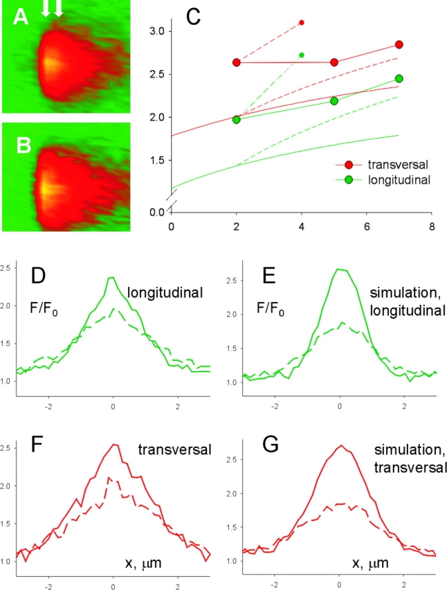
Postpeak expansion of sparks. (A and B) Averages of sparks of 2 ms rise time (range 1.51 to 2.5 ms) with longitudinal (A) or transversal scanning (B). The first arrow indicates time of peak and the second marks the postpeak expansion, especially clear in the longitudinal average (A). (C) Spatial widths of averages of events of different rise times, measured at their peak (large symbols) for longitudinal (green) or transversal scans. This plot demonstrates that the difference is large even at the shortest rise time, and is fractionally greatest there. The small dots, joined by dashed line to large symbols at 2-ms abscissa, represent the spatial width of the 2-ms rise time averages, measured in the first interval after the peak (hence the values are plotted at the 4-ms abscissa). Smooth continuous lines: evolution of FWHM in spark simulations (3 μm long cylindric source of 100 pA). Dashed lines starting at 2 ms: FWHM of simulated sparks when the source was closed after 2 ms. (D and F) Solid lines: spatial profile at the time of the peak (2 ms), dashed lines: 4-ms later. For the longitudinal scan (D, green), the fluorescence at locations near 2 μm from the center of the spark is higher in the later record. (E and G) Spatial profile at peak and 4 ms postpeak in simulations with the cylindric source open for 2 ms.

The continuous lines in that panel represent the evolution of FWHM in spark simulations assuming a 3-μm long cylindric source. The dashed lines starting at 2 ms represent the FWHM of simulated sparks when the source was closed after 2 ms. These functions have many qualitative features in common with the observations. The relative difference between widths is maximal initially, and decreases with open time. The width continues to increase upon source closure. The rate of this increase after closure is faster in the longitudinal scanned simulation.

Intriguingly, the simulations share with the data a qualitative difference, whereby in longitudinal scans, and at some distance from the source, the fluorescence after the peak may increase above the values at the time of the peak. This was illustrated for averages of 5-ms rise time in Fig. 5, E and F, and is shown for the averages of rise time 2 ms in Fig. 13, D and F. As before, the solid lines represent the profile at the time of the peak (2 ms), and the dashed lines the profile 4 ms later. For the longitudinal scan, the fluorescence at 2 μm is higher in the later profile. The feature is qualitatively reproduced in the simulations (Fig. 13, E and G).

In conclusion, it was necessary to assume an extensive source, of supraresolution length, to qualitatively reproduce the features of rat sparks. This assumption also explained naturally the dependence of width on scan orientation, and the singular temporal evolution of this difference. An alternative explanation for the transversal elongation of sparks, that diffusion coefficients are anisotropic, was not considered likely given the nearly isotropic properties of frog sparks. The intensity of current needed in the simulations (50–130 pA), together with estimates of unitary current from previous work (ranging from 0.5 pA, unpublished data; to 1.4 pA, Tinker et al., 1993) or current in embers estimated at 0.7 or 1.3 pA, yields a range of 35–260 for the number of channels involved.

While a 3-μm long source yielded an adequate simulation, other lengths, combined with changes in other parameters, could have worked as well. A length of 3 μm, however, is consistent with the large estimates of channel numbers reached above, fitting some 200 channels in a double row at 30 nm between channels. Although a single couplon (defined as the channels on one side of a junctional segment of T tubule; Stern et al., 1997) already constitutes a source of supraresolution length (∼1 μm in the rat; Franzini-Armstrong et al., 1999), a source anywhere close to 3 μm in length would require more than one couplon. The implications of these numbers are intriguing. In particular, the essentially synchronous activation of tens of channels over a large junctional area would require a specific synchronization mechanism, perhaps the allosteric interactions proposed to explain coupled gating in bilayer experiments (Marx et al., 1998). Further speculation would benefit from more precise determinations of source geometry, for example using video-rate confocal microscopy (e.g., Lacampagne et al., 1999; Brum et al., 2000), an approach currently in progress in our laboratory.

Differences with Current in Sparks of Frog Muscle

In studies of frog or mammalian heart muscle, it is becoming increasingly clear that sparks of different morphology and properties may be observed, depending on the conditions, and surely reflecting a variable number of participating channels (for review see Schneider, 1999; Ríos and Brum, 2002; see also Chandler et al., 2003). The present estimates of numbers of channels involved in mammalian muscle sparks are greater than the high-end estimates in frog sparks. This reflects the fact that mammalian sparks are remarkably wide, but paradoxically of lower amplitude than their frog counterparts. The lower amplitude probably does not reflect differences between channels (Mejía-Alvarez et al., 1999; Kettlun et al., 2000), but suggests a lower driving force (i.e., luminal SR [Ca²⁺]) in the rat.

Another difference is the presence of embers, caused in the rat by channels that remain open after termination of the spark proper. The failure of some channels to close could simply be a consequence of the greater numbers of channels involved in rat sparks. There are indications, however, that gating is very different in these two species. For instance, frog sparks appear to have no spontaneous embers (González et al., 2000a), whereas in voltage-clamped mammalian fibers we consistently fail to find sparks (Shirokova et al., 1998; Zhou et al., 2003). The fact that channels close synchronously in frog sparks (Lacampagne et al., 1999) has been taken as evidence of a powerful inhibitory control mechanism, which avoids excessive Ca²⁺ release and underlies the abrupt reduction in release that follows the early peak in global records under voltage clamp. Why this mechanism is less effective in the mammal remains a puzzle. In a worst case scenario, mammalian muscle embers may reflect unspecific damage by the permeabilization procedure. This, however, is contradicted by the observation of similar events in mechanically split mammalian fibers (Kirsch et al., 2001), and no embers in saponized frog fibers (González et al., 2000a). It seems more likely that embers in the rat reflect fundamental control differences, not yet understood, with frog muscle.

We set out to study sparks of mammalian muscle spurred by their channel endowment, simpler than that of the frog. Against the expectations we encountered a richer variety of events in the mammal, and sparks that involve possibly a greater number of channels. Therefore, several puzzles remain: why sparks of mammalian muscle are scarce, and have not been seen to occur under voltage control (Shirokova et al., 1998; Zhou et al., 2003); why do they involve a number of channels greater than in the frog (spanning perhaps a few microns of junction); and, finally, the reasons for the failures of termination (revealed by delayed closure of channels in trailing sparks) and the failures of activation (visible in the presence of sparks with leading embers, as well as lone embers that do not elicit sparks). Answering these questions should help understand the functional significance of the different endowment of Ca²⁺ release channels in mammals and amphibians, as well as their mutual interactions and controls.

References

- Baylor, S.M., W.K. Chandler, and M.W. Marshall. 1983. Sarcoplasmic reticulum calcium release in frog skeletal muscle fibres estimated from Arsenazo III calcium transients. J. Physiol. 344:625–666. [DOI] [PMC free article] [PubMed] [Google Scholar]
- Baylor, S.M., J. Peet, W.K. Chandler, and S. Hollingworth. 2000. Calcium sparks evoked by caffeine in intact frog skeletal muscle fibers. Biophys. J. 78:438a. [Google Scholar]
- Baylor, S.M., S. Hollingworth, and W.K. Chandler. 2002. Comparison of simulated and measured calcium sparks in intact skeletal muscle fibers of the frog. J. Gen. Physiol. 120:349–368. [DOI] [PMC free article] [PubMed] [Google Scholar]
- Block, B.A., T. Imagawa, K.P. Campbell, and C. Franzini-Armstrong. 1988. Structural evidence for direct interaction between the molecular components of the transverse tubule/sarcoplasmic reticulum junction in skeletal muscle. J. Cell Biol. 107:2587–2600. [DOI] [PMC free article] [PubMed] [Google Scholar]
- Brum, G., A. González, J. Rengifo, N. Shirokova, and E. Ríos. 2000. Fast imaging in two dimensions resolves extensive sources of Ca2+ sparks in frog skeletal muscle. J. Physiol. 528:419–433. [DOI] [PMC free article] [PubMed] [Google Scholar]
- Chandler, W.K., S. Hollingworth, and S.M. Baylor. 2003. Simulation of calcium sparks in cut skeletal muscle fibers of the frog. J. Gen. Physiol. 121:311–324. [DOI] [PMC free article] [PubMed] [Google Scholar]
- Cheng, H., W.J. Lederer, and M.B. Cannell. 1993. Calcium sparks: elementary events underlying excitation-contraction coupling in heart muscle. Science. 262:740–744. [DOI] [PubMed] [Google Scholar]
- Cheng, H., L.S. Song, N. Shirokova, A. González, E.G. Lakatta, E. Ríos, and M.D. Stern. 1999. Amplitude distribution of calcium sparks in confocal Images. Theory and studies with an automatic detection method. Biophys. J. 76:606–617. [DOI] [PMC free article] [PubMed] [Google Scholar]
- Cheung, H.C. 2002. Calcium-induced molecular and structural signaling in striated muscle contraction. Molecular Control Mechanisms in Striated Muscle Contraction. R.J. Solaro and R.L. Moss, editors. Kluwer Academic Publishers, Norwell, MA.
- Conklin, M.W., V. Barone, V. Sorrentino, and R. Coronado. 1999. Contribution of ryanodine receptor type 3 to Ca(2+) sparks in embryonic mouse skeletal muscle. Biophys. J. 77:1394–1403. [DOI] [PMC free article] [PubMed] [Google Scholar]
- Csernoch, L., J. Zhou, B.S. Launikonis, A. González, M.D. Stern, G. Brum, and E. Ríos. 2003. The effects of SO4 2−, a Ca2+-precipitating buffer, on Ca2+ sparks of mammalian and batrachian muscle. Biophys. J. 84:386A. 12524292 [Google Scholar]
- Delbono, O., and E. Stefani. 1993. Calcium transients in single mammalian skeletal muscle fibres. J. Physiol. 463:689–707. [DOI] [PMC free article] [PubMed] [Google Scholar]
- Felder, E., and C. Franzini-Armstrong. 2002. Type 3 ryanodine receptors of skeletal muscle are segregated in a parajunctional position. Proc. Natl. Acad. Sci. USA. 99:1695–1700. [DOI] [PMC free article] [PubMed] [Google Scholar]
- Flucher, B.E., A. Conti, H. Takeshima, V. Sorrentino. 1999. Type 3 and type 1 ryanodine receptors are localized at the triads of the same mammalian skeletal muscle fibers. J. Cell Biol. 146:621–630. [DOI] [PMC free article] [PubMed] [Google Scholar]
- Franzini-Armstrong, C., F. Protasi, and V. Ramesh. 1999. Shape, size, and distribution of Ca2+ release units and couplons in skeletal and cardiac muscles. Biophys. J. 77:1528–1539. [DOI] [PMC free article] [PubMed] [Google Scholar]
- García, J., and M.F. Schneider. 1995. Suppression of calcium release by calcium or procaine in voltage clamped rat skeletal muscle fibres. J. Physiol. 485:437–445. [DOI] [PMC free article] [PubMed] [Google Scholar]
- González, A., W.G. Kirsch, N. Shirokova, G. Pizarro, M.D. Stern, and E. Ríos. 2000. a. The spark and its ember. Separately gated local components of Ca2+ release in skeletal muscle. J. Gen. Physiol. 115:139–157. [DOI] [PMC free article] [PubMed] [Google Scholar]
- González, A., W.G. Kirsch, N. Shirokova, G. Pizarro, G. Brum, I.N. Pessah, M.D. Stern, H. Cheng, and E. Ríos. 2000. b. Involvement of multiple intracellular release channels in calcium sparks of skeletal muscle. Proc. Natl. Acad. Sci. USA. 97:4380–4385. [DOI] [PMC free article] [PubMed] [Google Scholar]
- Harkins, A.B., N. Kurebayashi, and S.M. Baylor. 1993. Resting myoplasmic free calcium in frog skeletal muscle fibres estimated with fluo-3. Biophys. J. 65:865–881. [DOI] [PMC free article] [PubMed] [Google Scholar]
- Hoel, P.G. 1971. Introduction to mathematical statistics. Fourth Edition. John Wiley & Sons, Inc., New York. 211–217.
- Hollingworth, S., C. Soeller, S.M. Baylor, and M.B. Cannell. 1999. In skeletal muscle fibres, a rise in myoplasmic calcium appears to speed the diffusion of fluo-3 by perturbing the equilibrium between protein-free and protein-bound indicator. J. Gen. Physiol. 114:11a. [Google Scholar]
- Hui, C.S., and W.K. Chandler. 1990. Intramembranous charge movement in frog cut twitch fibers mounted in a double Vaseline-gap chamber. J. Gen. Physiol. 96:257–298. [DOI] [PMC free article] [PubMed] [Google Scholar]
- Jiang, Y.H., M.G. Klein, and M.F. Schneider. 1999. Numerical simulation of Ca2+ sparks in skeletal muscle. Biophys. J. 77:2333–2357. [DOI] [PMC free article] [PubMed] [Google Scholar]
- Kettlun, C., A. González, W. Nonner, E. Ríos, and M. Fill. 2000. Ryanodine receptor (RyR) unitary current is greater in frog skeletal muscle than in mammalian heart. Biophys. J. 78:2576. [Google Scholar]
- Kirsch, W.G., D. Uttenweiler, and R.H.A. Fink. 2001. Spark- and ember-like elementary Ca2+ release events in skinned fibres of adult mammalian skeletal muscle. J. Physiol. 537:379–389. [DOI] [PMC free article] [PubMed] [Google Scholar]
- Klein, M.G., H. Cheng, L.F. Santana, Y.H. Jiang, W.J. Lederer, and M.F. Schneider. 1996. Two mechanisms of quantized calcium release in skeletal muscle. Nature. 379:455–458. [DOI] [PubMed] [Google Scholar]
- Klein, M.G., A. Lacampagne, and M.F. Schneider. 1999. A repetitive mode of activation of discrete Ca2+ release events (Ca2+ sparks) in frog skeletal muscle fibres. J. Physiol. 515:391–411. [DOI] [PMC free article] [PubMed] [Google Scholar]
- Lacampagne, A., C.W. Ward, M.G. Klein, and M.F. Schneider. 1999. Time course of individual Ca2+ sparks in frog skeletal muscle recorded at high time resolution. J. Gen. Physiol. 113:187–198. [DOI] [PMC free article] [PubMed] [Google Scholar]
- Launikonis, B.S., and D.G. Stephenson. 1997. Effect of saponin treatment on the sarcoplasmic reticulum of rat, cane toad and crustacean (yabby) skeletal muscle. J. Physiol. 504:425–437. [DOI] [PMC free article] [PubMed] [Google Scholar]
- Marks, A.R., P. Tempst, K.S. Hwang, M.B. Taubman, M. Inui, C. Chadwick, S. Fleisher, and B. Nadal-Ginard. 1989. Molecular cloning and characterization of the ryanodine receptor/junctional channel complex cDNA from skeletal muscle sarcoplasmic reticulum. Proc. Natl. Acad. Sci. USA. 86:8683–8687. [DOI] [PMC free article] [PubMed] [Google Scholar]
- Marx, S.O., K. Ondrias, and A.R. Marks. 1998. Coupled gating between individual skeletal muscle Ca2+ release channels (ryanodine receptors). Science. 281:818–821. [DOI] [PubMed] [Google Scholar]
- Mejía-Alvarez, R., C. Kettlun, E. Ríos, M. Stern, and M. Fill. 1999. Unitary Ca2+ current through cardiac ryanodine receptor channels under quasi-physiological ionic conditions. J. Gen. Physiol. 113:177–186. [DOI] [PMC free article] [PubMed] [Google Scholar]
- Ogawa, Y., N. Kurebayashi, and T. Murayama. 1999. Ryanodine receptor isoforms in excitation-contraction coupling. Adv. Biophys. 36:27–64. [DOI] [PubMed] [Google Scholar]
- Park, S., and R. Schowengerdt. 1983. Image reconstruction by parametric cubic convolution. Comp. Vision. Graphics Image Process. 23:256–265. [Google Scholar]
- Ríos, E., M.D. Stern, A. González, G. Pizarro, and N. Shirokova. 1999. Calcium release flux underlying Ca2+ sparks of frog skeletal muscle. J. Gen. Physiol. 114:31–48. [DOI] [PMC free article] [PubMed] [Google Scholar]
- Ríos, E., and G. Brum. 2002. Ca2+ release flux underlying Ca2+ transients and Ca2+ sparks in skeletal muscle. Front. Biosci. 7:d1195–d1211. [DOI] [PubMed] [Google Scholar]
- Schneider, M.F. 1999. Perspective: Ca2+ sparks in frog skeletal muscle: generation by one, some or many SR Ca2+ release channels? J. Gen. Physiol. 113:365–372. [DOI] [PMC free article] [PubMed] [Google Scholar]
- Shtifman, A., C.W. Ward, J. Wang, H.H. Valdivia, and M.F. Schneider. 2000. Effects of imperatoxin A on local sarcoplasmic reticulum Ca(2+) release in frog skeletal muscle. Biophys. J. 79:814–827. [DOI] [PMC free article] [PubMed] [Google Scholar]
- Shirokova, N., J. García, and E. Ríos. 1996. Ca2+ release from the sarcoplasmic reticulum compared in amphibian and mammalian skeletal muscle. J. Gen. Physiol. 107:1–18. [DOI] [PMC free article] [PubMed] [Google Scholar]
- Shirokova, N., J. García, and E. Ríos. 1998. Local calcium release in mammalian skeletal muscle. J. Physiol. 512:377–384. [DOI] [PMC free article] [PubMed] [Google Scholar]
- Shirokova, N., A. González, W.G. Kirsch, E. Ríos, G. Pizarro, M.D. Stern, and H. Cheng. 1999. a. Calcium sparks: release packets of uncertain origin and fundamental role. J. Gen. Physiol. 113:377–384. [DOI] [PMC free article] [PubMed] [Google Scholar]
- Smith, G.D., J.E. Keizer, M.D. Stern, W.J. Lederer, and H. Cheng. 1998. A simple numerical model of calcium spark formation and detection in cardiac myocytes. Biophys. J. 75:15–32. [DOI] [PMC free article] [PubMed] [Google Scholar]
- Sobie, E.A., K.W. Dilly, J. dos Santos Cruz, W.J. Lederer, and M.S. Jafri. 2002. Termination of cardiac Ca2+ sparks: an investigative mathematical model of calcium-induced calcium release. Biophys. J. 83:59–78. [DOI] [PMC free article] [PubMed] [Google Scholar]
- Soeller, C., and M.B. Cannell. 2002. Estimation of the sarcoplasmic reticulum Ca2+ release flux underlying Ca2+ sparks. Biophys. J. 82:2396–2414. [DOI] [PMC free article] [PubMed] [Google Scholar]
- Stern, M.D., G. Pizarro, and E. Ríos. 1997. Local control model of excitation-contraction coupling in skeletal muscle. J. Gen. Physiol. 110:415–440. [DOI] [PMC free article] [PubMed] [Google Scholar]
- Sun, X.P., N. Callamaras, J.S. Marchant, and I. Parker. 1998. A continuum of InsP3-mediated elementary Ca2+ signalling events in Xenopus oocytes. J. Physiol. 509:67–80. [DOI] [PMC free article] [PubMed] [Google Scholar]
- Sutko, J.L., and J.A. Airey. 1996. Ryanodine receptor Ca2+ release channels: does diversity in form equal diversity in function? Physiol. Rev. 76:1027–1071. [DOI] [PubMed] [Google Scholar]
- Takeshima, H., S. Nishimura, T. Matsumoto, H. Ishida, K. Kangawa, N. Minamino, H. Matsuo, M. Ueda, M. Hanaoka, T. Hirose, and S. Numa. 1989. Primary structure and expression from complementary DNA of skeletal muscle ryanodine receptor. Nature. 339:439–445. [DOI] [PubMed] [Google Scholar]
- Tinker, A., A.R. Lindsay, and A.J. Williams. 1993. Cation conduction in the calcium release channel of the cardiac sarcoplasmic reticulum under physiological and pathophysiological conditions. Cardiovasc. Res. 27:1820–1825. [DOI] [PubMed] [Google Scholar]
- Tsugorka, A., E. Ríos, and L. Blatter. 1995. Imaging elementary events of calcium release in skeletal muscle cells. Science. 269:1723–1726. [DOI] [PubMed] [Google Scholar]
- Uttenweiler, D., W.G. Kirsch, E. Schulzke, M. Both, and R.H. Fink. 2002. Model-based analysis of elementary Ca2+ release events in skinned mammalian skeletal muscle fibres. Eur. Biophys. J. 31:331–340. [DOI] [PubMed] [Google Scholar]
- Zhou, J., L. Csernoch, J. Yi, B. Launikonis, A. González, E. Ríos, and J. García. 2003. Repression of Ca2+ sparks by voltage sensors or other T tubule structures in mammalian muscle. Biophys. J. 84:386A. 12524292 [Google Scholar]
Associated Data
This section collects any data citations, data availability statements, or supplementary materials included in this article.