Calcium Regulation of Single Ryanodine Receptor Channel Gating Analyzed Using HMM/MCMC Statistical Methods

Abstract

Type-II ryanodine receptor channels (RYRs) play a fundamental role in intracellular Ca²⁺ dynamics in heart. The processes of activation, inactivation, and regulation of these channels have been the subject of intensive research and the focus of recent debates. Typically, approaches to understand these processes involve statistical analysis of single RYRs, involving signal restoration, model estimation, and selection. These tasks are usually performed by following rather phenomenological criteria that turn models into self-fulfilling prophecies. Here, a thorough statistical treatment is applied by modeling single RYRs using aggregated hidden Markov models. Inferences are made using Bayesian statistics and stochastic search methods known as Markov chain Monte Carlo. These methods allow extension of the temporal resolution of the analysis far beyond the limits of previous approaches and provide a direct measure of the uncertainties associated with every estimation step, together with a direct assessment of why and where a particular model fails. Analyses of single RYRs at several Ca²⁺ concentrations are made by considering 16 models, some of them previously reported in the literature. Results clearly show that single RYRs have Ca²⁺-dependent gating modes. Moreover, our results demonstrate that single RYRs responding to a sudden change in Ca²⁺ display adaptation kinetics. Interestingly, best ranked models predict microscopic reversibility when monovalent cations are used as the main permeating species. Finally, the extended bandwidth revealed the existence of novel fast buzz-mode at low Ca²⁺ concentrations.

INTRODUCTION

Type II calcium release RYR channels play a fundamental role in the intra cellular Ca²⁺ signaling dynamics of cardiac muscle cells that govern contractility of the heart. RYR channels are activated by a small Ca²⁺ influx through the surface membrane by a process known as Ca²⁺-induced Ca²⁺ release (CICR). The CICR process, an inherently self-regenerating process, is precisely controlled in cells. The regenerative feedback that counters the positive feedback of CICR is thought to depend on the cytosolic Ca²⁺ concentration (Fabiato, 1985). Since then, the cytosolic RYR Ca²⁺ regulation has been the subject of extensive research (Györke and Fill, 1993; Laver and Curtis, 1996; Schiefer et al., 1995; Sitsapesan et al., 1995; Zaradnková et al., 1999; Copello and Fill, 2002), and resent matter of debate (Fill et al., 2000; Lamb et al., 2000; Sitsapesan and Williams 2000).

Several models of single RYR channel gating have been developed to explain the RYRs role in the overall Ca²⁺ dynamics of cardiac muscle cells. These models, however, have been usually chosen and estimated by following rather phenomenological criteria in order to reproduce experimentally observed properties such as the Ca²⁺-dependent activation, inactivation (Zaradniková and Zahradník, 1995; Stern et al., 1999), adaptation (Cheng et al., 1995; Sachs et al., 1995; Keizer and Levine, 1996; Villaba-Galea et al., 1998; Fill et al., 2000), and modal gating—as well as the local RYR-mediated intracellular Ca²⁺ release events known as Ca²⁺ sparks (Jafri et al., 1998; Sobie et al., 2002; Villaba-Galea et al., 2002). Even in the presence of high quality data, model estimation and selection have only rarely been statistically addressed. For example, Saftenku et al. (2001) present a maximum likelihood approach that is subject to several drawbacks. The raw data is idealized by using standard threshold methods at a relatively limited bandwidth (i.e., 2 kHz). Second, models for particular visually identified gating modes are then separately estimated via maximum likelihood (Qin et al., 1996). This analysis heavily relies on the quality of the initial idealizations and the accuracy of the mode identification steps. This makes it subject to errors that are very difficult to statistically assess. Even more importantly, it does not reveal the connections between the identified modes and thus presents only a partial picture of the salient dynamics with limited predictive power.

This article presents a first step toward a statistical analysis of single type II RYRs at steady-state. The analysis provides some substantial benefits when compared with previously used approaches. First, the applicable bandwidth of the analysis is extended up to 10 kHz by the use of hidden Markov models (HMMs; see Michalek et al., 1999; Venkataramanan and Sigworth, 2002). Second, statistical inferences are made using a combination of Bayesian statistics and stochastic search methods (Markov chain Monte Carlo [MCMC]). These techniques have proven to be particularly well suited for complex estimation problems where the more commonly applied maximum likelihood–based approaches fail (Robert and Casella, 1999; Liu, 2001). The MCMC method not only provides a rich description of the modeling process but also a direct indication of where and why a particular model fails. More importantly, it allows us to directly assess the errors incurred at each estimation step, since all the estimates used throughout are endowed with a central limit theorem. The MCMC technique used here, namely a Gibbs sampler, is a generalization of the method described in Rosales et al. (2001) that allows us to consider the constraints imposed by the aggregation of states into conductance classes and the set of state interconnections. These techniques are similar in spirit to those of Ball et al. (1999) and Hodgson (1999); however, here the continuous gating of the channel is approximated by a discreetly sampled process, producing a less computationally intensive algorithm that is based on a solid probabilistic theory.

16 gating models were compared on this basis by analyzing three datasets containing the steady-state activity of single RYRs at 1, 10, and 100 μM Ca²⁺. The results obtained provide direct evidence for the existence of different Ca²⁺-dependent gating modes. The open/closed states associated with each mode were also identified. Additionally, gating schemes were used to predict the relaxation kinetics of single RYR channel response to Ca²⁺ step stimuli. The kinetic predictions for the top ranked schemes agree well with those that have been experimentally defined, showing that single RYRs respond transiently to sudden Ca²⁺ steps. Our results also demonstrate that gating follows detailed balance at the experimental conditions so far considered.

MATERIALS AND METHODS

2.1. Microsome Preparation

Heavy microsomes enriched in type II RYRs obtained from canine ventricular cardiac muscle (Tate et al., 1985) were reconstituted in planar lipid bilayers (Miller and Racker, 1976). Briefly, the tissue was kept in a saline solution (154 mM NaCl, 10 mM Tris-malate, pH 6.8) at a temperature of 4°C before being chopped and then homogenized. Heavy microsomes were obtained by differential centrifugation and then kept at −70°C in saline solution with 300 mM sucrose until used.

2.2. Reconstitution and Recording

Planar lipid bilayers were formed across a 150 μm hole in a Delrin cup. Bilayers were obtained with a mixture (50 mg/ml in decane) of phosphatidylcholine (PC) and phosphatidylethanolamine (PE) (Avanti Polar Lipids, Inc.) in a 7:3 relation. Bilayers with an electrical capacitance of 200–400 pF were used in our experiments. The microsomes were added to one side of the bilayer defined as cis. The other side, defined as trans, was held at virtual ground. The standard solution was 20 mM CsCH₃SO₃, 20 μM CaCl₂, 20 mM HEPES, pH 7.4. The fusion of the microsomes was promoted by mechanical stirring and an osmotic gradient (i.e., addition of 400 mM CsCH₃SO₃). The orientation of an incorporated RYR was such that their cytoplasmic side was in the cis compartment (i.e., defined by sidedness of ATP sensitivity). After channel incorporation, the trans CsCH₃SO₃ concentration was adjusted to 420 mM. The charge carrier was Cs+. All experiments were done at room temperature.

A patch clamp amplifier (Axopatch 200B; Axon Instruments, Inc.) was used to optimize single channel recording (Györke and Fill, 1993). The acquisition software (pClamp 6.0; Axon Instruments, Inc.) was run on a Pentium III computer controlling a 12-bit analogue/digital-digital/analogue converter (Axon Instruments, Inc.). Single-channel data were digitized at 100 kHz and filtered at 32 kHz. To reduce posterior computational effort, the data was digitally Gaussian filtered down to 10 kHz and sampled at 25 kHz. Long single RYR channel recordings (3×10⁶ samples each) were made at three different steady-state free Ca²⁺ concentrations (1, 10, and 100 μM cis). Free Ca²⁺ concentration was verified using a Ca²⁺ electrode.

2.3. Data Analysis

A representative single-channel recording at each Ca²⁺ concentration was selected for analysis. The baseline was corrected to account for any drift and other irregularities. The files were analyzed separately with each of the 16 gating models shown in Fig. 1 . The data was modeled by considering constrained HMMs and a combination of Bayesian statistics and MCMC methods. The most relevant aspects of these techniques together with a brief mention to further methods used are described bellow. A detailed account of the Bayes/MCMC framework is given in Rosales (2004).

Figure 1.

Gating models. O_i and C _i denote open and closed states, respectively, and M _i ^a,b, with i = 1, …, 16, corresponds to model labels with a for associated number of free parameters and b for their ranking as given by Table I. Scheme M ₁₀ was proposed by Zaradniková and Zahradník (1996), M ₁₂ by Villalba-Galea et. al (1998), M ₁₃ by McManus and Magleby (1991), M ₁₄ by Fabiato (1985), M ₇ by B.A. Suarez-Isla (personal communication), and M ₁₆ by Schiefer et al. (1995).

2.3.1. Constrained HMMs

Observations were modeled by using constrained HMMs. Briefly, the gating dynamics of single RYR channels were assumed to follow a discreetly time sampled homogeneous Markov process with a finite state space E = {1, 2, …, n}. States were further aggregated into two conductance classes O = {O ₁, …, O _v} and C = {C ₁, …, C _w}, with v + w = n and O _i and C _i denoting single states, hereafter labeled open and closed. Transitions between the states of this process are not directly observed. The data arising from bilayer experiments is inherently corrupted by additive noise, assumed o be independent and Gaussian distributed as a first approximation. The constraints on the HMM parameter space considered here are those induced by the topology of the associated graph of a gating mechanism and those inherent to the association of states into C and O. The parameters involved are the transition probabilities p _ij, grouped into a transition probability matrix P = [p _ij], for any i, j ε O, or C, the class conductance levels μ_C and μ_O, the class noise variances σ² _C and σ² _O, and finally the initial density for the hidden process Λ = [λ_i], i ε{O, C}. For convenience hereafter we write θ = (P, μ_C, μ_O, σ² _C, σ² _O, Λ).

2.3.2. Bayesian Treatment

Within this framework, the identification of a gating model from the raw data leads to the following well posed statistical tasks: (A) signal idealization, (B) parameter estimation, and (C) model selection. Statistical inferences concerning C are considered by using an asymptotic form of penalized ratio test, namely the Bayesian information criterion, whereas tasks A and B are considered from a Bayesian perspective. Let y denote a set of N observations y ₁, y ₂, … y _N, and z a particular realization z ₁, z ₂, …, z _N of the underlying process, i.e., z represents a sequence of states visited by the channel. Furthermore, let Z stand for the space of all possible state sequences, and Θ a subset of the Euclidean space formed by the set of all possible values for θ. For each gating mechanism denote by L(θ, z) the likelihood function,

(1)

defined as the joint probability for the occurrence of the data and a hidden realization, given a particular value for the parameters θ. Let φ(θ) denote the prior, a density that expresses belief or knowledge about the parameters before the observations have been examined. Then, following Bayes theorem, the joint posterior density for both unknowns θ and z, is

(2)

with

Estimates for model parameters, task B, are based on this density by integrating out z, for instance,

(3)

(4)

constitute unbiased estimates for the model parameters and their associated variances. The same argument also applies for estimates of the hidden sequence z by integration of θ, which then represents a solution to task A.

2.3.3. MCMC

Although there are clear theoretical advantages for the use of posterior based inferences over maximum likelihood based approaches in this setting, none of the integrals in Eqs. 2–4 can be evaluated directly. This occurs even for the simplest gating mechanism and regardless of the choice of φ(θ), due the complex structure of the HMM marginal likelihood L θ,z. Thus, the required integrals have to be evaluated numerically. This task is performed here by using MCMC methods, more precisely by using the Gibbs sampler initially described by Rosales et al. (2001) and further modified by Rosales (2004) in order to accommodate class constraints. The basic principle behind any MCMC algorithm is to perform Monte Carlo integration by drawing samples of the required posterior in Eq. 2, and then evaluating sample averages to approximate the expectations in Eqs. 3 and 4. More precisely, in the current setting, the Gibbs sampler generates a sequence of random variables (θ ^u, z ^u), u = 1,2, …, m, by running a Markov chain for a long time, such that in the limit as m→ +∞, the pair (θ ^m, z ^m) is asymptotically distributed according to the target distribution π. In fact, for the constrained HMM outlined above, the Gibbs sampler converges toward π from any arbitrary starting point (θ ¹, z ¹). These and other regularity properties of the sampler have been formally established in Rosales (2004).

An example of the output generated by analyzing a small data segment with model M ₃ of Fig. 1 is shown in Fig. 2 . This example shows how the sampler performs a random walk on two of the model parameters θ, namely on σ_O2 ² and σ_C2 ². After a few steps the walk finally stays within a boundary that corresponds to a region of maximum posterior probability for (σ_O2 ²,σ_C2 ²). This figure also presents the output generated for the hidden process shown as a randomly chosen set of idealized traces, z ^u, each one generated at a given iteration of the MCMC run. Well identifiable features are actually recovered in almost all iterations, whereas very brief events appear only in some of the sampled realizations.

Figure 2.

MCMC output example. (Top left) Brief segment of RYR activity at 10 kHz. Horizontal axis is 0.1 s long and vertical axis stretches over 5 pA. (Bottom left) Ensemble of 10 MCMC-sampled realizations of the hidden process obtained by analyzing the data at the top with gating scheme M ₃ of Figure 1. The first five realizations are within the first 1,000 iterations of the sampler and the last 5 are from the remaining 1,000 iterations. (Right) Trajectory followed by 2,000 iterations of the MCMC sampler on the class variances σ² _O (x-axis), σ² _C (y-axis) plotted as solid lines. Dashed lines represent 12 contour levels for a surface proportional to the HMM log posterior computed by varying (σ² _O,σ² _C) and leaving all other model parameters fixed at their posterior estimates.

Formally, due to convergence toward π, Monte Carlo estimates for the posterior mean and standard deviation of θ (Eqs. 3 and 4) are, respectively, the empirical averages of the obtained sequence (θ ^u), i.e.,

(5)

(6)

for some 1 < b < m and G = m − b + 1.

The use of these equations may be illustrated by the following example. Let Q* = [k _ij* for i,j ε{O,C} be a transition rate matrix for the process z estimated from the data and associated to P as

(7)

with exp as the matrix exponential and δ as the sampling period of the acquisition system. It should be emphasized that Q* is not the infinitesimal generator, Q = [k _ij], of the hidden process, but rather a rate matrix associated to the limiting time resolution δ. Hereafter, however, for notational convenience we write Q for Q* and k _ij for k*_ij, the elements of Q*. If the continuous process is sampled fast enough, i.e., if

then, following standard theory (see for instance Eq. 7 of Colquhoun and Hawkes, 1995a),

(8)

A posterior estimate for the observed transition rate matrix and its standard deviation follow immediately from these equations and Eqs. 5 and 6, namely

(9)

and

(10)

Convergence of the sampler, and hence estimation of b in Eqs. 5 and 6, was assessed by the Raftery-Lewis and Heidelberger-Welch tests, both implemented in R (http://cran.r-project.org) or SPlus by the BOA program (Bayesian Output Analysis program; Version 1.0.0 for S-PLUS and R; http://www.public-health. uiowa.edu/boa/). MCMC runs were started at an arbitrary initial point θ ¹ εΘ for each model. The same values were used for any of the three Ca²⁺ conditions and each model (see Fig. 1). The initial hidden realization, z ¹, was drawn from the initial density Λ¹ and the initial probability matrix P ¹. A weak informative prior for θ was considered (see Rosales et al., 2001).

2.3.4. Density Estimates

Posterior dwell-time density estimates based on the MCMC sampled realizations, (z ^u), for each model were computed by using optimal nonparametric kernel density estimation methods instead of standard log-binned histograms (Rosales et al., 2002). Where indicated, dwell-time densities were also calculated directly from the Q matrix estimates (Colquhoun and Hawkes, 1995b). Interclass state correlations were visually inspected by computing the dependency-difference plot introduced by Magleby and Song (1992). Estimates for the posterior parameter densities were also computed by using kernel methods and the MCMC output (θ ^u). In this case estimates were obtained by following Bowman and Azzalini (1997).

2.3.5. Model Choice

Models are compared by using the Bayes information criterion (BIC), see for instance Gelfand and Dey (1994), which introduces a penalty according to the total number of free parameters and the length of the data record. For any mechanism this is given by

(11)

with N _θ as the total number of associated free parameters and L as the marginal likelihood,

evaluated at some θ^· that maximizes its value. Here we have chosen the posterior mean estimate, i.e., θ^· = _π θ. From Eq. 1,

(12)

This quantity is efficiently computed, once _π θ is obtained from the MCMC runs, by using Baum's forward procedure (Baum et al., 1970). Finally, if the data y is partitioned into s independent segments of lengths N ₁, N ₂, …, N _s and the likelihood for the ith segment is denoted by L _i, then from Eq. 11 the BIC takes the form

(13)

A model is preferred over another if its BIC as defined by Eq. 13 is smaller.

2.3.6. Evolution Toward Equilibrium

Let η(kδ) = [η _i(kδ)], i ε{C,O}, be a n-dimensional row vector denoting the state occupation density at any time k=1,2, …, for δ > 0. Relaxation toward the equilibrium distribution, η(∞), is given by

(14)

with η(0) as an arbitrary initial distribution (see theorem 1.13 of Norris, 1997). This relation describes the evolution for the δ-discretisation of the continuous time process (see theorem 2.1.1 of Norris, 1997). In fact, the continuous time version for Eq. 14 is standard and may be found in the current context at several places by setting P ^kδ = exp(Qkδ) (see Eq. 19 of Colquhoun and Hawkes, 1995b). The open probability P _o as a function of kδ, is thus obtained via Eq. 14 by adding the entries in η that involve open states, i.e.

(15)

In this study, however, the scope of Eq. 15 is restricted to the evaluation of η(kδ) by using only one of the estimated Q at a time, representing one of the Ca²⁺ conditions considered experimentally.

2.3.7. Online Supplemental Material

The MCMC sampler used in this study was written in ANSI C and is freely available under the GNU license as online supplemental material (available at http://www.jgp.org/cgi/content/full/jgp.200308868/DC1). Code is distributed with documentation concerning compilation and running examples. Compilation under various platforms including SUN Sparks running Solaris 8, and several Pentiums with Linux and most Windows versions was made with gcc (http://gcc.gnu.org). Precompiled binaries may be available upon request by writing to the first author. Code and documentation for dwell-time kernel estimates is also available as online supplemental material. Kernel estimates for the parameter posterior marginals were computed from the MCMC output by using the sm library implemented in R and conforming to Bowman and Azzalini (1997). Simple plots were made with gnuplot (http://www.gnuplot.info) and others including surfaces with R. All Q matrix computations were made by using Maple 7 (Waterloo Maple, Inc.). When run on the dataset at 10 μM Ca²⁺ (3.051 × 106 samples) with scheme M ₃ (9 states and 29 free parameters), each iteration of the sampler took 17.8 s on a Dell Precision 330 with a 1.4 GHz Pentium 4 processor.

RESULTS

3.1. Model Comparison

Results obtained by analyzing single RYR channel data collected at three different Ca²⁺ concentrations with the gating schemes shown in Fig. 1 are summarized in Table I . This table presents the values for the negative of the marginal log likelihood evaluated at the posterior mean estimates for the associated parameters at each Ca²⁺ concentration. Models are ordered from top to bottom according to their BIC ranking, as determined by Eq. 13. Simple inspection suggests that the information in the data strongly supports model complexity, as shown by the difference of 20,787.47 BIC units between the best ranked model (scheme M ₃) and the worst one (scheme M ₁₅). Complexity in this context is related to the total number of free parameters. The following general topological properties of the graph associated to a mechanism may be inferred from Table I:

TABLE I.

Model Ranks for the Gating Schemes in Fig. 1

Model	1 μM Ca2+	10 μM Ca2+	100 μM Ca2+	BIC/2
M 3	5,017,201.39	4,622,527.19	8,198,295.779	17,839,341.024
M 1	5,016,912.009	4,622,752.312	8,198,978.954	17,839,959.940
M 13	5,017,478.084	4,622,561.437	8,198,668.95	17,839,979.734
M 2	5,017,461.44	4,622,935.34	8,198,278.653	17,839,992.098
M 8	5,017,074.007	4,622,573.273	8,199,085.133	17,840,049.078
M 6	5,018,281.31	4,622,578.398	8,198,451.814	17,840,355.774
M 7	5,017,204.83	4,622,840.487	8,199,158.714	17,840,384.489
M 4	5,017,889.128	4,621,674.612	8,200,051.146	17,841,067.758
M 5	5,019,861.823	4,622,046.314	8,198,188.557	17,841,413.359
M 12	5,019,369.695	4,623,852.529	8,201,986.333	17,846,525.222
M 11	5,019,316.927	4,623,867.826	8,210,510.667	17,854,875.878
M 9	5,022,059.333	4,626,502.531	8,206,993.875	17,856,872.404
M 10	5,022,645.991	4,626,611.635	8,207,225.326	17,857,390.997
M 16	5,021,177.153	4,630,058.04	8,206,816.649	17,858,596.676
M 14	5,021,616.988	4,630,147.467	8,206,814.655	17,859,214.742
M 15	5,021,768.858	4,630,484.904	8,207,424.004	17,860,177.191

Column values for the 1, 10, and 100 μM Ca²⁺ conditions are the marginal −log(likelihood) evaluated at the posterior mean for the parameters (see Eq. 12). Posterior means are computed via Eq. 5 from the MCMC output by discarding the first 2,500 samples out of a total of 3,000. The column entitled “BIC/2” represents half the penalized total given by the BIC computed by using Eq. 13.

(1) RYR channel gating schemes with three open states are preferred over those with two open states. Two open state schemes are preferred over those with one open state. Three open states would be consistent with the RYR channel experimental results published by Sitsapesan and Williams (1994) and Saftenku et al. (2001).

(2) RYR gating schemes with two communicating open states are preferred, see for example M ₁ and M ₂.

(3) RYR gating schemes with a hexagonal cycle of states have higher BIC values than those with smaller cycles.

(4) The best RYR gating schemes with three open states, except for scheme M ₁₃, share a common motif that includes states O ₂, O ₃, C ₄, C ₅, and C ₆. Schemes, such as M ₅ and M ₆, lacking this structure are ranked low.

(5) RYR gating schemes with more than two consecutive closed states not communicating with an open state at the left of the cycle such as C ₁, C ₂, and C ₃ in M ₄ and M ₅ are also heavily penalized.

(6) Table I also suggest the existence of more than four pathways between the open and the closed class. Interestingly, more than one pathway is necessary to explain modal RYR channel gating, an experimentally observed feature of single RYR channels (Zaradniková and Zahradník, 1995; Copello et al., 1997).

Results and predictions for the top ranked models with three open and six closed states are very similar and thus will not be detailed separately here. Instead, we will turn our attention below to the best ranked model, namely RYR gating scheme M ₃.

3.2. Q Matrix Estimates

Estimates for the Q matrices at each Ca²⁺ concentration constitute the basis for all further descriptions and predictions of the dynamics of single RYR channel behavior here. Fig. 3 displays the sampled values of the transition rates between communicating states of mechanism M ₃ for each Ca²⁺ condition, plotted against the MCMC iteration. These rates were obtained from the sampled probabilities by using Eq. 8. This figure also presents the sampled values for the variance of the open and the closed levels, σ_{O 2} and σ_{C 2}, respectively.

Figure 3.

MCMC samples for the Q matrix and the noise variances σ² _O, σ² _C for scheme M ₃. Samples for the transition rates of communicating states of scheme M ₃ are plotted against the number of iterations, when analyzing data at 1 μM Ca²⁺ (top left), 10 μM Ca²⁺ (top right), and 100 μM Ca²⁺ (bottom left). The plot at the bottom right presents the samples for the class noise variances at 10 μM Ca²⁺.

Simple inspection suggests that rate estimates for 1 and 100 μM Ca²⁺ have converged after ∼1,000 iterations. Convergence takes perhaps longer for the data at 10 μM Ca²⁺ (see Fig. 3, top right). Convergence at each concentration was quantitatively assessed by the Raftery-Lewis and Heidelberger-Welch tests (see Table II) . The latter being more conservative than the first one indicates a convergence period lag of 1,500 iterations. Based on this information, the first 2,500 iterations were discarded and only the remaining 500 iterations were considered for further inferences.

TABLE II.

MCMC Convergence Assessment

	R-L			H-W
[Ca2+]	1 μM	10 μM	100 μM	1 μM	10 μM	100 μM
C1→C2	72	15	4	1,500	1,500	1,200
C2→C1	18	42	9	1,500	1,500	1,500
C2→C3	168	54	32	1,500	1,500	1,500
C2→O3	36	70	240	1,500	1,500	1,500
C3→C2	155	196	30	1,500	1,500	1,200
C3→O1	4	25	235	1,500	1,500	1,200
C4→C5	56	60	360	1,500	1,500	1,500
C4→O2	35	84	35	1,500	1,500	1,500
C4→O3	96	20	70	1,500	1,200	1,200
C5→C4	72	36	330	1,500	1,500	1,500
C6→O2	119	80	16	1,500	1,500	1,500
O1→C3	16	15	300	300	1,500	1,500
O1→O2	6	20	36	300	1,500	1,200
O2→C4	63	30	20	900	1,500	1,500
O2→C6	60	56	144	300	1,500	300
O2→O1	6	32	48	300	600	900
O3→C2	15	8	238	1,500	1,200	1,500
O3→C4	30	10	650	1,500	1,500	1,500

Estimates for the MCMC sampler burn in period (b in Eq. 5) obtained via the Raftery-Lewis (R-L) and the Heidelberger-Welch (H-W) tests for the transition rates of scheme M ₃ at three Ca²⁺ conditions.

The posterior mean and standard deviation for each rate, computed by using the last 500 samples via Eqs. 9 and 10, are shown in Table III . Few posterior marginal density estimates for some individual parameters are shown in Fig. 4 . They were computed directly from the MCMC output according to Bowman and Azzalini (1997).

TABLE III.

Q Matrix Estimates for Scheme M₃

	1 μM Ca2+	10 μM Ca2+	100 μM Ca2+
C1→C2	1.4258160 ± 0.04962111	0.0706565 ± 0.0080813	0.0309433 ± 0.0057437
C2→C1	1.0481374 ± 0.0267937	0.0238650 ± 0.0050402	0.0021193 ± 0.0004699
C2→C3	0.7015191 ± 0.0332045	0.2704625 ± 0.0333583	0.0228213 ± 0.0031189
C2→O3	0.0352840 ± 0.0018467	0.3641249 ± 0.0137403	0.3958404 ± 0.0100573
C3→C2	4.3244367 ± 0.24452607	0.4015897 ± 0.0267361	0.9611583 ± 0.0897372
C3→O1	0.0010442 ± 0.0006090	0.0096410 ± 0.0015421	4.4228817 ± 0.2084783
C4→C5	1.8593915 ± 0.2305158	0.0306152 ± 0.0214537	0.4156589 ± 0.0244401
C4→O2	0.2292084 ± 0.0290348	0.8407021 ± 0.0611324	0.0746159 ± 0.00327612
C4→O3	0.4643987 ± 0.04477838	0.0908996 ± 0.0062598	0.9488903 ± 0.01257812
C5→C4	0.5778158 ± 0.04520021	0.3246417 ± 0.1324921	2.5809008 ± 0.13811970
C6→O2	24.5557880 ± 0.15655333	3.8166455 ± 0.1845010	1.8312432 ± 0.02034814
O1→C3	0.0021002 ± 0.00150776	0.0235335 ± 0.0026635	0.5574192 ± 0.02015974
O1→O2	0.0460808 ± 0.00468395	0.2075024 ± 0.0099914	0.1843850 ± 0.01264873
O2→C4	0.8825940 ± 0.03636925	0.2341961 ± 0.0151709	0.2774037 ± 0.01046813
O2→C6	3.9963179 ± 0.10731264	0.2614998 ± 0.0156431	2.6105679 ± 0.028012529
O2→O1	0.1324386 ± 0.01503245	0.0806450 ± 0.0058234	0.0406819 ± 0.00331926
O3→C2	0.5483176 ± 0.03331976	1.3070995 ± 0.0165400	0.4294915 ± 0.03175259
O3→C4	0.7087304 ± 0.03225781	0.0792834 ± 0.0053881	3.5881837 ± 0.03938660

Posterior mean value for Q and associated posterior standard deviation (±) for: 1, 10, and 100 μM Ca²⁺. Mean and standard deviation values are computed from the MCMC output by using Eq. 9, and taking the last 500 iterations out of 3,000. Diagonal entries of the transition rate matrix are not shown (k _ii = Σ_{j ≠ i} − k _ij for all i,j ε{O,C}). All mean values are expressed in ms⁻¹.

Figure 4.

Parameter posterior marginals. Density estimates for few selected parameters: k _C2C3 (A), k _C3O1 (B), k _O2C4 (C), k _O3C4 (D), σ² _O (E), and σ² _C (F). Estimates were computed by taking the last 500 samples for the MCMC run at 10 μM Ca²⁺ for scheme M ₃ (see Figure 3), and the routines provided by Bowman and Azzalini. Gray shaded reference bands indicate the region where the estimate is likely to lie if the data were normally distributed. Bars at the bottom show the actual MCMC samples.

In general, the rates leaving short-lived states with small occupancy probability (see Tables V and IV below) have relatively high variances. An example is provided by C ₆ at 1 μM Ca²⁺. Rates leaving long-lived states with larger occupancy probabilities, such as C ₁ at 1 μM Ca²⁺, have relatively smaller variances.

TABLE V.

Single-state Time Constants and Ca²⁺ for Scheme M₃

Ca2+	τC1	τC2	τC3	τC4	τC5	τC6	τO1	τO2	τO3
μM	ms	ms	ms	ms	ms	ms	ms	ms	ms
1	53.8077	.4502	.1888	.3337	7.4782	.0407	21.2984	.1995	.7955
10	15.4694	5.3341	1.1258	1.0231	3.2319	.262	5.3206	1.6144	.7213
100	32.4956	2.4008	.1856	1.2086	.3132	.5461	1.354	.3411	.2489

The ith time constant, τ_i, is found by taking the inverse of the ith eigenvalue of −Q. The Q matrices each Ca²⁺ condition used here are those shown in Table III.

The presence of multiple maxima in the posterior marginals (Fig. 4, A and C), and thus almost surely on the respective likelihood projections, should warn against the naive use of maximum likelihood methods for HMMs. This may include the use of standard deviations obtained from the likelihood curvature at “the maximum” (see Qin et al., 2000).

3.3. Single-state Ca²⁺-induced Changes

Straightforward computations with the Q matrix estimates lead to the associated stationary probabilities of being at each state and the expected time spent in each state. These quantities, shown in Tables IV and V , when considered together allow us to draw a detailed picture for the Ca²⁺ induced changes. For this, the next section starts with a description of the RYR channel gating modes present at 1 μM Ca²⁺ and follows then by identifying the states involved in each mode.

TABLE IV.

Equilibrium Densities and Ca²⁺ for Scheme M₃

	C1	C2	C3	C4	C5	C6	O1	O2	O3
η1(∞)	.29646	.40328	.06542	.03963	.12754	.00168	.02973	.0103	.02596
η10(∞)	.09013	.26684	.18034	.06187	.00583	.01514	.08467	.22102	.07414
η100(∞)	.00806	.11761	.00293	.40861	.06581	.15602	.02345	.10944	.10809

The densities at each condition were computed from the Q estimates shown in Table III as η(∞) = u(SS ^T)⁻¹, with S as a n × n + 1 matrix formed by augmenting the Q estimate with a column of ones, S ^T as the transpose of S, and u as a n-column vector with each element equal to 1 (see for example Eq. 17 of Colquhoun and Hawkes [1995b]).

Gating modes are clearly visible at 1 μM Ca²⁺. Fig. 5 displays two representative single RYR channel records illustrating at least three gating modes. The first of them, labeled G _l, consists of long openings interrupted by brief closures. The second, named G _z, consists of brief openings followed by brief closures and finally the third mode, named G _o, is formed by brief openings followed by long shut periods. As shown in Fig. 5, open sojourns in G _l and G _z are grouped in clusters forming burst-like behavior. G _l has previously been identified in single RYR channel studies as a mode of high open probability named H gating mode, and G _o as a mode with low probability named L gating mode (Zaradniková and Zahradník, 1995, 1996; Armisén et al., 1996). G _z is not mentioned in these earlier references. The states participating in each of the G _l, G _z, and G _o modes and the closed periods between them may be identified directly by inspecting the last MCMC sampled realizations for the hidden process (z ^u). However, as mentioned above, this may also be done by considering the single state time constants and occupation probabilities (see Tables V and IV) obtained from the Q matrix estimates.

Figure 5.

Gating modes at 1 mM Ca²⁺. Two segments of data used at 1 μM Ca²⁺ showing three distinct gating modes labeled as: G _z, G _o, and G _l. The vertical range for both traces is 3.5 pA, whereas the horizontal is 160 ms. Data was filtered down to 2 kHz with a digital Gaussian filter for display purpose.

At 1 μ Ca²⁺ the channel spends most of its time at the C ₁ and C ₂ states, which account for the long closed sojourns between the G _l and G _z modes. From the C ₂ state, the channel may then enter the O ₃ state generating a brief opening. From the O ₃ state, it may enter the C ₄ state forming events corresponding to the G _o gating mode. Also from the C ₂ state, via C ₃, the RYR channel may also (very rarely) enter the O ₁ sate generating a long lasting opening. These long openings may be followed by transitions toward the O ₂ state (brief openings) and subsequently to the C ₄ or C ₆ states (brief closings) forming bursts of channel activity characteristic of the G _l gating mode. From either the O ₁ or O ₂ states, G _l bursts are terminated either via O ₂→C ₄→O ₃→C ₂ or O ₁→C ₃→C ₂. The appearance of the G _z gating mode is associated with transitions of the form O ₃→C ₄↔O ₂↔C ₆, where the C ₆ state is responsible for the very fast closed characteristic of this mode. From the rates leaving C ₂ shown in Table III, there are 23 more transitions per unit of time toward the C ₃ state, the intermediate state for the initiation of a G _l gating mode bursts, than those for the O ₃ state that starts the G _o gating mode. Despite this, G _l gating mode bursts are quite rare when compared with the occurrence of the G _o gating mode. This is due to an extremely low rate for the transition from the C ₃ to O ₁ state. The appearance of the G _z or G _o modes is governed by the rates leaving the state C ₄ to the O ₂ and O ₃ states, respectively. Note that transitions to the O ₃ state are twice as frequent as those to the O ₂ state. This explains the apparent excess of the occurrence of G _o mode over G _z bursts. These results suggest the following gating mode frequency relations, G _l G _z G _o. At this Ca²⁺ concentration the open probability for the channel is 0.06599. A schematic view of the modes described above and their participating states is summarized in Fig. 6 .

Figure 6.

Gating modes for scheme M ₃ at 1 mM Ca²⁺. The scheme highlights the more critical set of transitions for each gating mode in model M ₃.

At 10 μM Ca²⁺ the channel tends to leave C ₁ and C ₂, which are shorter than at 1 μM Ca²⁺, and starts spending more time in states C ₃ and C ₄, both intermediately lived. Consequently, the inter -burst time is reduced, and this makes burst-like behavior less apparent. The channel also spends more time in all three open states, elevating the open probability to 0.37983. At this Ca²⁺ concentration, the preferred open state is now O ₂. This state is shorter than the most probable open state at 1 μM Ca²⁺ (O ₁), which was responsible for long open sojourns during G _l bursts. This accounts for a considerable reduction in the total G _l open time. Bursts of type G _z are ∼9 times more frequent than sojourns in the G _o mode, whereas the proportion between the G _l and G _o gating modes is more equally distributed in contrast to the situation at 1 μM Ca²⁺.

Finally, at 100 μM Ca²⁺ the channel now prefers to stay at C ₄, a briefly lived closed state, and mostly frequents two intermediate brief open states, O ₂ and O ₃. This accounts for a decrease in the open probability, which is now 0.24098, and also to the disappearance of long openings and closings between bursts.

3.4. Dwell Time Density Estimates

Apart from the mean times and the probabilities at each state, further insights into the Ca²⁺-induced changes in single RYR channel activity may be gained by inspection of the relative frequencies of visits to particular states. These are shown in Fig. 7 , which presents the log dwell-time densities for the sojourns in the open and closed classes together with their single-state components. Overall densities and components were computed by using the spectral decomposition of Q (Colquhoun and Hawkes, 1995b) and the estimates shown in Table III. At 1 μM Ca²⁺ both open and closed densities show two clearly defined maxima. Fast events in the open class (Fig. 7 A) constituted by sojourns in O ₂ and O ₃ are about five times more frequent than slow sojourns in O ₁. A high frequency of transitions to O ₃ accounts for most openings in the G _o mode. The closed class (Fig. 7 B) presents quite frequent fast and slow events corresponding to sojourns in C ₆ and C ₁, C ₅, respectively. The presence of multiple maxima in both classes at 10 μM Ca²⁺ is not as apparent as for 1 Ca²⁺. This accounts for a partial disappearance of modal behavior. At this Ca²⁺ concentration (10 μM) the maximum for the open class is slightly shifted toward the right (Fig. 7 C) when compared with the mayor maximum at 1 Ca²⁺. Furthermore, O ₃ is now the most frequent open state, being then closely followed by O ₂ and O ₁. The most frequent states for the closed class (Fig. 7 D) are C ₆ and C ₄. Provided the gating modes have still the same meaning as at 1 μM Ca²⁺, both plots at 10 μM Ca²⁺ suggest the following mode frequency relations G _l < G _o < G _z. Finally at 100 μM Ca²⁺ (Fig. 7, E and F) the densities for both classes have essentially a single well-defined maximum. This corresponds to a complete disappearance of modal behavior. At this concentration (100 μM Ca²⁺), the single-state frequency proportions are roughly the same as for 10 μM Ca²⁺. These results suggest that a mayor change in the single state frequencies occurs only around 1–10 μM Ca²⁺.

Figure 7.

Single-class dwell-time densities. (Left column) Log dwell-time densities for the sojourns in the open class of scheme M ₃ at 1 (plot A), 10 (C), and 100 (E) μM Ca²⁺. (Right column) Densities for the dwell times in the closed class of scheme M ₃ at 1 (plot B), 10 (D), and 100 (F) μM Ca²⁺. Solid lines are the class densities, whereas dashed lines present their single-state components. Densities are shown by taking their square root.

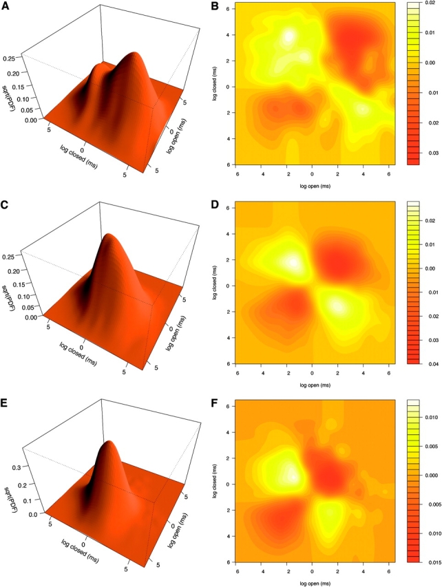
The univariate single-class densities suggest the existence of Ca²⁺-dependent RYR channel modal gating. However, direct evidence for this is only provided by the adjacent open-closed sojourn correlations. These are presented in Fig. 8 , which displays a MCMC posterior estimate for the log open-closed dwell time densities and their derived dependency-difference plots. Dwell-time densities were computed by using only the last five MCMC sampled realizations of the hidden process. Use of more MCMC realizations did not appreciably improve these estimates. A gating mode corresponds (in principle) to the existence of a peak (or maximum) in the joint density estimate. Inspection of Fig. 8 (top) suggests the existence of two modes at 1 Ca²⁺. These modes appear to gradually merge into a single mode at progressively higher Ca²⁺ concentrations (10–100 μM Ca²⁺). Such a simple visual inspection of the joint density plots can be misleading. Specific correlations between communicating states may be shown instead via dependency-difference plots. At 1 μM Ca²⁺ Fig. 8 B suggests the existence of at least three maxima (yellow to faint yellow contoured regions in the range of 0.0 to 0.04). The first of them corresponds to fast open-closed events associated to the G _z mode and is located at the bottom left corner of the plot. Another clearly identified maximum corresponds to long openings followed by brief closures (G _l mode). This is located in the region that starts at (2,0) at stretches horizontally to about (5,0). A third relatively minor maximum corresponds to intermediate openings followed by somewhat longer closings (G _o mode). This one may be identified with a region that starts at (0,0) and stretches vertically up to about (0,4).

Figure 8.

Joint open-closed dwell-time densities and dependence differences. Joint densities for MCMC-sampled open-closed sojourns of scheme M ₃ at 1 (surface A), 10 (C), and 100 (E) μM Ca²⁺. Surfaces show the square root of the density estimate. Dependence difference plots shown as contours for 1 (contour B), 10 (D), and 100 μM Ca²⁺ (F).

This analysis also suggests there is a major change in modal gating characteristics between 1 to 10 μM Ca²⁺. At 10 Ca²⁺ the dependency-difference plots show evidence of two maxima instead of three (Fig. 8 D). One of these corresponds to brief openings followed by intermediate length closures. The other corresponds to intermediate openings followed by short closures. This pattern is also evident at 100 μM Ca²⁺ (Fig. 8 F). However, correlations at 100 μM Ca²⁺ are much smaller (note contour level scales). This analysis presents direct evidence for RYR channel modal gating and reveals how it changes at different Ca²⁺ concentrations.

3.5. Filter and Threshold at 2 kHz

This section presents a standard filter and threshold analysis at 2 kHz. The purpose of this exercise is to illustrate the significance of the extended bandwidth analysis obtained by using the HMM approach. The data used for the MCMC analysis was first filtered down to 2 kHz with a digital Gaussian filter. The filtered data was then idealized by using a standard half amplitude threshold. The resulting dwell-time list was then finally used for dwell-time kernel density estimation. Fig. 9 presents the single-class estimates, whereas Fig. 10 shows the joint density for adjacent open-closed sojourns at each Ca²⁺ concentration.

Figure 9.

Single-class dwell-time densities at 2 kHz. (Left column, solid lines) Log dwell-time densities for the sojourns in the open class for the data filtered at 2 kHz at 1 (plot A), 10 (C), and 100 (E) μM Ca²⁺. (Right column, solid lines) Densities for the dwell times in the closed class for the data filtered at 2 kHz at 1 (plot B), 10 (D), and 100 (F) μM Ca²⁺. Dashed lines represent the density estimates obtained via MCMC (see Fig. 7). Densities are shown by taking their square root.

Figure 10.

Filtered joint open-closed dwell time densities and dependence-differences. Joint densities for 2 kHz filtered data at 1 surface (A), 10 (C), and 100 (E) μM Ca²⁺. Surfaces show the square root of the density estimate. Dependence-difference plots shown as contours for 1 (contour B), 10 (D), and 100 (F) μM Ca²⁺.

Both figures show several differences when compared, respectively, to Figs. 7 and 8. Simple inspection shows that changes are quite dramatic at 1 μM Ca²⁺. Indeed, Fig. 9, A and B, shows that fast events in both the open and the closed classes have disappeared almost entirely at 2 kHz. As a consequence both densities are shifted to the right. This effect is more markedly appreciated in the closed class (Fig. 9 B), since at 10 kHz this density presents one of the fastest components identified with sojourns in state C ₆ (see Fig. 7 B and also Table V). Fig. 9 B also presents smaller probability values than Fig. 7 B for the slowest events. This effect is due to noise events that still cross the threshold at 2 kHz and break long shut periods. A comparison of the joint density in Fig. 10 A against the one in Fig. 8 A also suggests the disappearance of fast adjacent open-closed sojourns that form the G _z gating mode. This is confirmed by comparison of the dependence-differences in Figs. 10 B and 8 B. The disappearance of G _z modifies the correlation pattern observed at 1 μM Ca²⁺, which is actually inverted when compared against the one in Fig. 8 B. Fig. 10 B presents two regions of positive correlations that correspond to intermediary fast and slow open-closed sojourns, much like the pattern found for 10 and 100 Ca²⁺ (see Figs. 10, D and E, and 8, D and E).

3.6. Reversibility

Reversibility can be evaluated by the Kolmogorov's criterion for Markov chains with cycles (see Eq. 1.22 in Kelly, 1979) using the Q matrix estimates. Let a ₁, a ₂, …, a _n−1, a _n denote the states involved in the cycle of a particular gating mechanism. Gating is reversible if the transition rates in the cycle satisfy

(16)

For the cycle of scheme M ₃, the clockwise product of the six rates involved at 1 μM Ca²⁺ is 6.9 × 10⁻⁶. The product of the six rates in the opposite direction product is 6.6 × 10⁻⁶. For 10 μM Ca²⁺ the products are 1.5 × 10⁻⁵ and 1.8 × 10⁻⁵ respectively. For 100 μM Ca²⁺ these products are 2.1 × 10⁻³ and 2.3 × 10⁻³. These results present direct evidence for the reversibility of single RYR channel gating dynamics at the experimental conditions tested here. They are also consistent with Fig. 11 . It should be emphasized that none of the cyclic models used so far considered reversibility constraints for the values of the transition probabilities pij. The results of these tests thus provide strong evidence in favor of time-reversible gating as a genuine feature of the data.

Figure 11.

Graphical reversibility test. Reversibility tests for 1 (A), 10 (B), and 100 (C) μM Ca²⁺. Each surface was obtained as described, but directly from the kernel estimates shown in Fig. 8, A, C, and E, respectively. The significance of the deviations from 0, and hence violation of detailed balance, was computed by following Song and Magleby (1994). Let K ⁺ _ij and K ⁻ _ij denote the joint dwell-time kernel estimates obtained by taking adjacent open-closed and closed-open dwell time pairs (the open-closed kernels for each Ca²⁺ concentration are shown in Fig. 8, A, C, and E). The ij indices represent the coordinates in the kernel evaluation grid. The observed differences are significant at the 5% level if U = (2χ²)^1/2 − (2D − 1)^1/2 > 1.96, with χ² = Σ_ij [(K ⁺ _ij − K ⁻ _ij)²/(K ⁺ _ij + K ⁻ _ij)], and D the total number of ij-pairs where K ⁺ _ij + K ⁻ _ij > 5 × 10⁻². The test gave U = −0.10293 for A, U = −4.10542 for B and U = 0.313686 for C.

3.7. Response to Sudden Ca²⁺ Steps

The response of RYR channels to fast Ca²⁺ changes can be evaluated by computing the relaxation toward equilibrium of the probability of being in the open class, P _o. Here, we present the response of mechanism M ₃ to instantaneous changes in the Ca²⁺ concentration from 0 to 1, 10, or 100 μM Ca²⁺. The predicted response of a single RYR channel was computed using Eq. 15, and considering several initial densities that represent possible candidates of the resting state. These were chosen by assigning different probability values to the closed states and 0 to any open state. For all the Ca²⁺ steps and initial conditions considered, Fig. 12 shows that the P _o rapidly peaks and the slowly relaxes toward a new equilibrium. This pattern of single RYR channel behavior has been experimentally observed (Györke and Fill, 1993; Valdivia et al., 1995). Closer inspection of the plots in Fig. 12 shows that the rising phase of the responses is strongly dependent on the resting condition.

Figure 12.

Relaxation of scheme M ₃ to instantaneous Ca²⁺ steps. Plots A, B, and C present the relaxation toward the equilibrium for the probability in the open class (P _o) as a response to a instantaneous step to 1 (plot A), 10 (B), and 100 (C) μM Ca²⁺. Single traces at each condition represent the relaxation obtained via Eq. 15 for different initial densities. Let the entries of this density, η(0), be ordered as η(0) = [η_{C 1}(0), …, η_{C 6}(0),η_{O 1}(0), …, η_{O 3}(0)]. The solid lines in A, B, and C present the response for η(0) = [0,0,0,0.3,0.7,0,0,0,0], dashed for η(0) = [0,0,0,0, 1,0,0,0,0], dotted for η(0) = [0,0,0.1,0.2,0.7,0,0,0,0], dot-dashed for η(0) = [0,0,0.2, 0.3,0.5,0,0,0,0], long-dashed for η(0) = [0,0,0.4,0.3,0.3,0, 0,0,0], and finally two-dashed for η(0) = [0,0.01,0.49,0.3, 0.2,0,0,0,0]. Plot in D represents the time course for the three Ca²⁺ steps from 0 to 1, 10, and 100 μM that generated, respectively, A, B, and C.

3.8. MCMC Method Reliability

To test the reliability of the MCMC method, simulated single-channel data was obscured by adding random noise. θ and z were then estimated and compared to their original values. To this end, two synthetic datasets were generated assuming two different Ca²⁺ conditions. One synthetic dataset was generated using Q matrix estimates for the M ₃ model at 1 μM Ca²⁺. The specific rate constants used for the M ₃ model are presented in Table III. The second synthetic dataset was generated using Q-matrix estimates for the M ₁₀ model at 10 μM Ca²⁺. The specific rate constants used for the M ₁₀ model are presented below (in ms⁻¹).

Synthetic datasets with N = 2 × 10⁶ samples were generated by sampling at δ = 0.04 ms. The following parameters were set to mimic those estimated from real data; μ_C = 0.9985, μ_O = 2.6784 and σ² _C = σ² _O = 0.5955. The synthetic dataset were then processed using the Gibbs sampler. The Gibbs sampler was run for 3,000 iterations with different gating schemes. Convergence in each case was diagnosed as described in Section 2.3.3. Only the last 1,000 iterations were used for estimation.

For the synthetic dataset generated using the M ₃ model, the Gibbs sampler was run with four different gating schemes (M ₃, M ₂, M ₇, and M ₁₄). The actual Q-matrix samples for the M ₃ model are shown in Fig. 13 . This figure also contains results obtained from the real single channel data for comparison (also see Fig. 3).

Figure 13.

Q matrix samples for M ₃. Plot A shows the MCMC samples obtained for the real dataset at 1 μM Ca²⁺ (same as Fig. 3). Plot B presents the MCMC samples obtained from a 2,000,000 point dataset generated by using the Q matrix estimates obtained from the run in A (see Table III).

The BIC/2 factors as given by Eq. 13 for M ₃, M ₂, M ₇, and M ₁₄ are, respectively, 3,227,097.713, 3,227,131.317, 3,227,155.629, and 3,798,851.394. This means that the rank order of best-fit models was M ₃ > M ₂ > M ₇ > M ₁₄. In the M ₃ model case, the estimates generated for μ_C, μ_O, and σ² _C and σ² _O were 0.9979, 2.679, and 0.5961, respectively. The estimates for the rate constants (in ms⁻¹) are listed below.

For the synthetic dataset generated using the M ₁₀ model, the Gibbs sampler was also run for with four different gating schemes M ₁, M ₃, M ₁₀, and M ₁₁. The rate constant estimates (in ms⁻¹) are listed below.

The BIC/2 factors for the M ₁, M ₃, M ₁₀, and M ₁₁ models are 2,571,612.52, 2,571,723.112, 223,01,276.171 and 345,101.05, respectively. This means that the rank order of best-fit model was M ₁₀ > M ₁₁ > M ₁ > M ₃.

In both cases, the estimated rate constants are similar to the original values used to generate the simulated datasets. Thus, the HMM-MCMC analysis performed reasonably well under noise conditions similar to those found experimentally. Further, the BIC values show that the method was also able to accurately choose the correct model.

3.9. Reproducibility of the Best-fit RYR Channel Model Prediction

Model selection was done using real single RYR channel data collected at three different cytosolic Ca²⁺ concentrations. Here, the reproducibility of the model selection is evaluated using real single RYR channel recordings at a single cytosolic Ca²⁺ concentration (100 μM). These recordings were collected from two different RYR channels. For each recording, the Gibbs sampler was used to generate estimates of rate constants and BIC values. Two complete rate prediction and BIC value sets from this analysis are provided here to illustrate the degree of channel-to-channel variability present. Rate estimates obtained from the analysis of the previously presented data collected at 100 μM Ca²⁺ are presented in Table VI . Estimates obtained from the analysis of another long (6.84 × 10⁶ samples) single RYR channel recording at 100 μM Ca²⁺ are presented in Table VII . The experimental conditions in which both of these recording were done were exactly the same.

TABLE VI.

Kinetic Parameters for Three Different Top-ranked Models for a Channel at 100 μM Ca²⁺

M 2		M 3		M 13
C1→C2	0.041 ± 0.007	C1→C2	0.031 ± 0.006	C1→C2	0.056 ± 0.008
C2→C1	0.002 ± 0.0003	C2→C1	0.002 ± 0.0005	C2→C1	0.006 ± 0.001
C2→O1	0.105 ± 0.005	C2→C3	0.023 ± 0.003	C2→C3	1.055 ± 0.049
C2→O3	0.887 ± 0.025	C2→O3	0.396 ± 0.01	C3→C2	0.235 ±0.015
C3→O1	1.816 ± 0.022	C3→C2	0.961 ± 0.09	C3→C4	0.052 ± 0.003
C3→O2	0.028 ± 0.003	C3→O1	4.423 ± 0.208	C3→O1	0.996 ± 0.008
C4→C5	0.627 ± 0.042	C4→C5	0.416 ± 0.024	C4→C3	1.687 ± 0.079
C4→O2	0.015 ±0.002	C4→O2	0.075 ± 0.003	C4→C5	1.971 ± 0.106
C4→O3	0.854 ± 0.043	C4→O3	0.949 ± 0.013	C4→O2	3.032 ± 0.078
C5→C4	1.736 ± 0.097	C5→C4	2.581 ± 0.138	C5→C4	0.209 ± 0.009
C6→O2	5.189 ± 0.204	C6→O2	1.831 ± 0.02	C5→O3	1.666 ± 0.017
O1→C2	0.289 ± 0.013	O1→C3	0.557 ± 0.02	O1→C3	3.951 ± 0.019
O1→C3	2.627 ± 0.03	O1→O2	0.184 ± 0.013	O1→O2	0.0006 ± 0.0007
O2→C3	0.146 ±0.013	O2→C4	0.2777 ± 0.01	O2→C4	1.023 ± 0.019
O2→C4	0.137 ± 0.01	O2→C6	2.611 ± 0.028	O2→O1	0.001 ±0.001
O2→C6	0.438 ± 0.016	O2→O1	0.041 ± 0.003	O2→O3	0.002 ± 0.002
O3→C2	2.188 ± 0.053	O3→C2	0.429 ± 0.031	O3→C5	3.16 ± 0.025
O3→C4	1.790 ± 0.052	O3→C4	3.588 ± 0.039	O3→O2	0.0003 ± 0.0004

Values of the rate constants for state transitions and their standard deviations are given for the channel described in Section 3.3. Three (M ₂, M ₃, and M ₁₃) of the five top ranked models are compared.

TABLE VII.

Kinetic Parameters for Three Different Top-ranked Models for a Channel at 100 μM Ca²⁺

M2		M3		M13
C1→C2	0.0076 ± 0.001	C1→C2	0.63 ± 0.177	C1→C2	0.006 ± 0.001
C2→C1	0.0005 ± 0.0001	C2→C1	1.567 ± 0.362	C2→C1	0.0009 ± 0.0002
C2→O1	0.3997 ± 0.004	C2→C3	0.006 ± 0.004	C2→C3	0.934 ± 0.036
C2→O3	0.0281 ± 0.001	C2→O3	0.017 ± 0.006	C3→C2	0.44 ± 0.025
C3→O1	0.0006 ± 0.0008	C3→C2	0.003 ± 0.002	C3→C4	0.001 ± 0.0009
C3→O2	1.265 ± 0.061	C3→O1	2.899 ± 0.075	C3→O1	0.742 ± 0.01
C4→C5	0.304 ± 0.027	C4→C5	0.377 ± 0.014	C4→C3	0.003 ± 0.002
C4→O2	0.039 ± 0.002	C4→O2	0.029 ± 0.001	C4→C5	0.003 ± 0.003
C4→O3	1.078 ± 0.016	C4→O3	0.692 ± 0.008	C4→O2	0.956 ± 0.011
C5→C4	1.024 ± 0.049	C5→C4	0.852 ± 0.024	C5→C4	0.323 ± 0.089
C6→O2	4.584 ± 0.347	C6→O2	0.938 ± 0.01	C5→O3	2.623 ± 0.099
O1→C2	2.827 ± 0.025	O1→C3	0.5 ± 0.011	O1→C3	2.513 ± 0.019
O1→C3	0.0005 ± 0.0005	O1→O2	0.177 ± 0.008	O1→O2	0.109 ± 0.006
O2→C3	0.321 ± 0.02	O2→C4	0.057 ± 0.003	O2→C4	1.465 ± 0.014
O2→C4	0.103 ± 0.005	O2→C6	1.449 ± 0.016	O2→O1	0.067 ± 0.005
O2→C6	0.228 ± 0.018	O2→O1	0.083 ± 0.005	O2→C3	0.085 ± 0.006
O3→C2	0.056 ± 0.003	O3→C2	0.001 ± 0.0003	O3→C5	0.551 ± 0.023
O3→C4	1.68 ± 0.018	O3→C4	2.552 ± 0.018	O3→O2	0.108 ± 0.02

Values of the rate constants for state transitions and their standard deviations are given for the channel described in Section 3.9. Three (M ₂, M ₃, and M ₁₃) of the five top ranked models are compared.

These tables contain the rate constant estimates and associated standard deviations for only three of the top ranked models (M ₂, M ₃, and M ₁₃). These rate estimates where computed by taking only the last 500 of 3,000 iterations of the Gibbs sampler. Convergence in each case was diagnosed as described in Section 2.3.3. Particular rate estimates obtained from the two channels are not identical. As expected, the natural biological variability between channels does impose variability in the absolute values of the predicted time constants. However, the relative magnitudes of the particular rate constants are relatively consistent between the channels. To illustrate the consistency in magnitude, the coefficient of variation between the rate constants estimations for all transitions in one of the top ranked models (M ₂) are plotted in Fig. 14 .

Figure 14.

Coefficient of variation for each rate constant of model M ₂ for different set of data. The coefficient of variation (standard deviation expressed as a percentage of the mean) was computed for model 2 using data extracted from Tables VI and VII. The average change of the rate constants for different channels was 53%.

The BIC values obtained from the different analysis sets were used to rank the models. The BIC values for each analysis set are presented in Tables I and VIII . In each case, the BIC values were then used to rank order the best-fit models for each analysis set. The best-fit rank orders for the two analysis sets are compared in Table VIII. The rank orders from both analysis sets contain the sequence M ₄ > M ₁₂ > M ₉ > M ₁₀ > M ₁₆ >M ₁₄ > M ₁₅. More importantly, the top five best-fit models were M ₂, M ₃, M₅, M ₆, and M ₁₃ although not in exactly the same order. Note that the BIC value differences between these top five ranked models in most cases are quite small.

TABLE VIII.

BIC Ranking for a Channel at 100 μM Ca²⁺

Model	BIC/2-channel A	Model	BIC/2-channel B
M 5	8,198,188.557	M 2	10,526,296.294
M 2	8,198,278.653	M 13	10,526,519.547
M 3	8,198,295.779	M 3	10,526,296.294
M 6	8,198,451.814	M 6	10,526,590.176
M 13	8,198,668.95	M 5	10,526,752.767
M 1	8,198,978.954	M 8	10,527,500.14
M 8	8,199,085.133	M 7	10,527,582.358
M 7	8,199,158.714	M 1	10,528,876.02
M 4	8,200,051.146	M 11	10,530,168.661
M 12	8,201,986.333	M 4	10,530,343.001
M 9	8,206,814.655	M 12	10,530,508.683
M 10	8,206,816.649	M 9	10,537,283.837
M 16	8,206,993.875	M 10	10,537,822.011
M 14	8,207,225.326	M 16	10,538,386.957
M 15	8,207,424.004	M 14	10,538,715.39
M 11	8,210,510.667	M 15	10,540,334.274

The comparison for two different channels A (channel described in Section 3.3) and B (channel described in Section 3.8) is shown. The first five models (M ₂, M ₃, M ₅, M ₆, and M ₁₃) are common for the two channels (see Section 3.9).

DISCUSSION

Detailed knowledge about the dynamics of single RYR channel Ca²⁺ regulation is required to understand the role these molecules play in the local control of excitation-contraction coupling (Stern, 1992). Despite extensive research, many questions regarding the mechanisms that govern RYR channel gating remain unanswered. Several Markov models for the gating of single RYRs have been proposed. Typically, models have been selected and parameters estimated rather heuristically, usually by imposing a strong set of constraints that turn them into essentially a self-fulfilling prophecy (see Sachs et al., 1995; Zaradniková and Zahradník, 1996; Villaba-Galea et al., 1998; Sobie et al., 2002). These approaches end up simply showing that the selected model can reproduce a particular RYR channel attribute (e.g., modal gating, adaptation, and/or inactivation) with little (if any) statistical evaluation. The principal objective here is to infer single RYR properties directly from data by setting a minimum number of constraints on the model structure. By doing so, we have considered sixteen gating models, six of them previously reported in the literature. Statistical inferences were made from Bayesian perspective by using MCMC. The next sections summarize the implications of our findings and discuss their limitations.

4.1. Extended Bandwidth

The HMM approach applied here extends the analysis of single-channel data to relatively high bandwidths. This is particularly important for fast gating channels like the RYRs (Zaradniková et al., 1999). Here, the HMMs were applied to analyze single RYR channel data at 10 kHz. This analysis was directly compared with standard filter and threshold at 2 kHz. Although the same datasets were analyzed, there was a dramatic difference in outcome (see Figs. 6–9). Filtering at 2 kHz removed a considerable proportion of very fast events, shifted distributions, and obscured (in some cases eliminated) observed correlations between adjacent open-closed events. The filtering distortion was most marked at low Ca²⁺ levels (i.e., 1 μM) and generated a completely different pattern of single-channel gating. This is an important finding. It introduces new information concerning the physiological relevance of fast events of single RYR channels at low Ca²⁺ concentrations specifically.

4.2. Reversibility

Both the surface plots at Fig. 11 and the Kolmogorov's criterion for cycles for the Q matrix estimates show that RYR channels gate in detailed balance. It should be noted that this result is not in contradiction with recent evidence that supports irreversible gating when Ca²⁺ is the main diffusing species (Wang et al., 2002). Furthermore, this agrees and reinforces results of Rengifo et al. (2002) and Villaba-Galea et al. (2002), which propose the dissipation of the Ca²⁺ gradient as the source of free energy that keeps the system out of time reversibility.

4.3. Modal Gating and Adaptation

The steady-state Ca²⁺ sensitivity of single RYR channels is well established (Zaradniková and Zahradník, 1995, 1996; Armisén et al., 1996). The dynamics of single RYR channel Ca²⁺ regulation is not (Copello and Fill, 2002). It is clear from numerous studies that single RYR channels display rapid activation in response to a fast Ca²⁺ elevation (Györke and Fill, 1993; Zaradnková et al., 1999). In some studies, channel activity peaks and then spontaneously decays following the fast Ca²⁺ elevation. The spontaneous decay was originally termed adaptation (Györke and Fill, 1993) and was particularly interesting because it occurred at Ca²⁺ concentrations that do not inactivate the RYR channel under steady-state conditions. The spontaneous decay (i.e., adaptation) has now been attributed to a Ca²⁺ and time dependent modal gating shift (Zaradniková and Zahradník, 1995, 1996; Villaba-Galea et al., 1998; Györke, 1999; Zaradniková et al., 1999; Fill et al., 2000).

Interestingly, the highest ranked gating model selected from steady-state single-channel data predicts a spontaneous decay after a fast-step Ca²⁺ elevation (see Fig. 12). This is interesting because there has been vigorous debate about whether or not this is possible. In the original adaptation studies (Györke and Fill, 1993), the applied Ca²⁺ elevation had a very fast (1 ms) overshoot at its leading edge. At first, this very fast Ca²⁺ overshoot was not considered to play a role in the much slower spontaneous decay (Velez et al., 1997). However, the possibility that the fast Ca²⁺ overshoot may actually generate the slow spontaneous decay was quickly forwarded (Lamb and Stephenson, 1995; Lamb et al., 2000; Sitsapesan and Williams, 2000). Here, a spontaneous decay occurs in the absence of fast Ca²⁺ overshoot. The analysis here supports the notion that this spontaneous decay is generated by a Ca²⁺- and time-dependent modal gating shift (see below). The analysis here also suggests that a fast Ca²⁺ overshoot may indeed accelerate the initial transition into the open configuration, but will not have an impact on single RYR channel behavior after that.

As mentioned above, single RYR channels display rapid activation in response to a fast Ca²⁺ elevation (Zaradnková et al., 1999). There is no dispute concerning this RYR channel attribute. The model with highest BIC score, selected here from steady-state data, predicts a Ca²⁺ activation rate similar to those that have been experimentally defined (Györke and Fill, 1993; Valdivia et al., 1995; Velez et al., 1997). Not surprisingly, the Ca²⁺ activation rate depends on the initial conditions that exist before the fast Ca²⁺ change.

Several studies have detailed the Ca²⁺-dependent modal gating of single RYR channels (Armisén et al., 1996; Zaradniková and Zahradník, 1996; Zaradnková et al., 1999). Again, the highest ranked model predicts the existence of Ca²⁺-dependent modal gating (see Fig. 8). The analyses here show that the Ca²⁺ dependence of modal gating is steepest at relatively low Ca²⁺ concentrations (≈1 μM). This corresponds to the Ca²⁺ concentration range over which adaptation is experimentally observed (Fill et al., 2000). This also supports the notion that adaptation (i.e., the spontaneous decay) is due to a Ca²⁺- and time-dependent modal gating shift. As initially proposed by Zaradniková and Zahradník (1995) the Ca²⁺-dependent modal shift hypothesis rests essentially on two basic assumptions: (a) an increase of Ca²⁺ should favor transitions out of states with high P _o, but (b) at resting conditions Ca²⁺ can only bind to transitions that lead to these states. These conditions still remain to be fully demonstrated. The analysis in Zaradniková et al. (1999) and the one presented here are consistent with the first point; however, none of them provides the means for the identification of the specific Ca²⁺-dependent transitions.

4.4. MCMC Method Reliability and Robustness of the Fit

The reliability of the MCMC method was tested by simulating two different synthetic datasets using the parameters fitted for two different models under two different cytosolic Ca²⁺ concentrations. Then noise was added to recordings simulated from the Q matrices and the HMM MCMC formalism was used for analyze the simulated data (Section 3.8). Excitingly, the analysis again correctly retrieves the model used to produce the data for the synthetic datasets.

To test the Robustness of our methods, two different channels under similar ionic conditions (100 μM free cytosolic Ca ²⁺ concentration) were analyzed using the HMM MCMC formalism. In Section 3.9 the model selection for two different channels and the rate constants are compared. Although the model selection rankings are note identical, the best first five models were the same for all the channels. It is not surprising that the ranking for different channels is not identical, mostly because the natural biological variability between channels. Nevertheless, BIC values for these top models are very similar. In addition, when the fitted Q matrices for the same model (M ₂) and two different datasets were compared (Fig. 14) the rate constants for each transition were not exactly the same but were in the same order. This difference could be explained again by the variability of the biological samples.

4.5. Future Directions

A key limitation of the approach applied here is the estimation of a separate Q matrix for each Ca²⁺ condition. The simultaneous estimation of a single common matrix should significantly improve its statistical properties; moreover, this should lead to the identification the Ca²⁺-dependent transitions of a gating scheme. The latter would certainly clarify several aspects in the Ca²⁺-dependent modal shift hypothesis. Finally, a single Q matrix with well-identified Ca²⁺-dependent transitions would enclose all the necessary information for predicting the Ca²⁺-dependent dynamic properties of single RYR channels. This includes the response to any imaginable Ca²⁺ waveform allowing comparison of predicted channel behavior with the myriad of experimental results that have been reported (Györke and Fill, 1993; Sitsapesan et al., 1995; Laver and Curtis, 1996; Zaradnková et al., 1999). More importantly, it would allow prediction of single RYR channels to the nonstationary Ca²⁺-regulatory environment that exists in living cells.

To make inferences by considering data at several Ca²⁺ concentrations simultaneously one has to be able introduce constraints for the rates, such that the involved states become well-defined occupancy sites for Ca²⁺. For instance, one would generally like to set k _ij = α_ij[Ca²⁺], where α_ij is the rate constant that results in the case [Ca²⁺] = 1 μM, if k _ij is to be expressed in μM × s⁻¹. Unfortunately, these constraints do not translate in a simple manner to P and hence into the standard HMM formulation. The problem may be illustrated by considering an expansion of the exponential form which relates P and Q (see Eq. 7), namely,

(17)

with I as the identity matrix. P may well be obtained from Q by simple matrix operations, but a simple change in one entry of Q takes a rather complicated algebraic form in P. Work in progress, however, shows that it is indeed possible to sample Q directly by using hybrid MCMC moves that include Metropolis-Hastings steps (Robert and Casella, 1999; Liu, 2001) inside the Gibbs sampler used here. This approach is highly promising, both in theory and in practice since it borrows many of the properties of the Gibbs sampler so far used.

In any case, unifying views of the Ca²⁺-regulatory dynamics of RYRs will certainly continue to stimulate the research of thorough quantitative analytical approaches and innovative experimental strategies.

References

- Armisén, R., J. Sierralta, P. Vélez, D. Naranjo, and B.A. Súarez-Isla. 1996. Modal gating in neuronal and skeletal muscle ryanodine-sensitive Ca2+ release channels. Am. J. Physiol. 271:C144–C153. [DOI] [PubMed] [Google Scholar]
- Ball, F.G., Y. Cai, J.B. Kadane, and A. O'Hagan. 1999. Bayesian inference for ion channel gating mechanisms directly from single channel recordings, using Markov chain Monte Carlo. Proc. Roy. Soc. Lond. A. 455:2879–2932. [Google Scholar]
- Baum, L.E., T. Petrie, G. Soules, and N. Weiss. 1970. A maximization technique ocurring in the statistical analysis of probabilistic functions of Markov chains. Ann. Math. Stat. 41:164–171. [Google Scholar]
- Bowman, A.W., and A. Azzalini. 1997. Applied Smoothing Techniques for Data Analysis. Oxford Statistical Science Series, 18. Clarendon Press, Oxford, UK.
- Cheng, H., M. Fill, and H. Valdivia. 1995. Models of Ca2+ release channels adaptation. Science. 267:2009–2010. [DOI] [PubMed] [Google Scholar]
- Colquhoun, D., and A.G. Hawkes. 1995a. Principles of the stochastic interpretation of ion-channel mechanisms. Single-channel Recording. B. Sackmann and E. Neher, editors. Plenum, New York. 397–482.
- Colquhoun, D., and A.G. Hawkes. 1995b. A Q-Matrix cookbook. Single-channel Recording. B. Sackmann and E. Neher, editors. Plenum, New York. 589–633.
- Copello, J.A., S. Barg, H. Onoue, and S. Fleischer. 1997. Heterogeneity of Ca2+ gating of skeletal muscle and cardiac ryanodine receptors. Biophys. J. 73:141–156. [DOI] [PMC free article] [PubMed] [Google Scholar]
- Copello, J.A., and M. Fill. 2002. Ryanodine receptor calcium release channels. Physiol. Rev. 82:893–922. [DOI] [PubMed] [Google Scholar]
- Fabiato, A. 1985. Time and calcium dependence of activation and inactivation of calcium-induced release of calcium from the sarcoplasmic reticulum of a skinned canine cardiac Purkinje cell. J. Gen. Physiol. 85:247–289. [DOI] [PMC free article] [PubMed] [Google Scholar]
- Fill, M., A. Zahradnková, C.A. Villalba-Galea, I. Zahradnk, A.L. Escobar, and S. Györke. 2000. Ryanodine receptor adaptation. J. Gen. Physiol. 116:873–802. [DOI] [PMC free article] [PubMed] [Google Scholar]
- Gelfand, A.E., and D.K. Dey. 1994. Bayesian model choice: asymptotics and exact calculations. J. Roy. Stat. Soc. Ser. B. 56:501–514. [Google Scholar]
- Györke, S. 1999. Ca2+ spark termination: inactivation and adaptation may be manifestations of the same mechanism. J. Gen. Physiol. 114:163–166. [DOI] [PMC free article] [PubMed] [Google Scholar]
- Györke, S., and M. Fill. 1993. Ryanodine receptor adaptation: control mechanism of Ca2+-induced Ca2+ release in heart. Science. 260:807–809. [DOI] [PubMed] [Google Scholar]
- Hodgson, M.E.A. 1999. A Bayesian restoration of an ion channel signal. J. Roy. Stat. Soc. B. 61:95–114. [Google Scholar]
- Jafri, M.S., J.J. Rice, and W.L. Winslow. 1998. Cardiac Ca2+ dynamics: the roles of ryanodine receptor adaptation and sarcoplasmic reticulum load. Biophys. J. 74: 1149–1168. [DOI] [PMC free article] [PubMed] [Google Scholar]
- Keizer, J., and L. Levine. 1996. Ryanodine receptor adaptation and CICR-dependent Ca2+ oscillations. Biophys. J. 71:3477–3487. [DOI] [PMC free article] [PubMed] [Google Scholar]
- Kelly, F. 1979. Reversibility and Stochastic Networks. Wiley Series in Probability and Mathematical Statistics. John Wiley & Sons, New York.
- Lamb, G.D., D.R. Laver, and D.G. Stephenson. 2000. Questions about adaptation in ryanodine receptors. J. Gen. Physiol. 116:883–890. [DOI] [PMC free article] [PubMed] [Google Scholar]
- Lamb, G.D., and D.G. Stephenson. 1995. Activation of ryanodine receptors by flash photolisis of caged Ca2+. Biophys. J. 68:946–948. [DOI] [PMC free article] [PubMed] [Google Scholar]
- Laver, D.R., and B.A. Curtis. 1996. Response of ryanodine receptor channels to Ca2+ steps produced by rapid solution changes. Biophys. J. 71:732–741. [DOI] [PMC free article] [PubMed] [Google Scholar]
- Liu, J.S. 2001. Monte Carlo Strategies in Scientific Computing. Springer Verlag, New York.
- Magleby, K.L., and L. Song. 1992. Dependency plots suggest the kinetic structure of ion channels. Proc. R. Soc. Lond. B. Biol. Sci. 249:133–142. [DOI] [PubMed] [Google Scholar]
- McManus, D.B., and K.L. Magleby. 1991. Accounting for the Ca2+-dependent kinetics of single large-conductance Ca2+-activated K+ channels in rat skeletal muscle. J. Physiol. 443:739–777. [DOI] [PMC free article] [PubMed] [Google Scholar]
- Michalek, S., H. Lerche, M. Wagner, N. Mitrovic, M. Schiebe, F. Lehmann-Horn, and J. Timmer. 1999. On identification of Na+ channel gating schemes using moving-average filtered hidden Markov models. Eur. Biophys. J. 28:605–609. [DOI] [PubMed] [Google Scholar]
- Miller, C., and E. Racker. 1976. Ca2+-induced fusion of fragmented sarcoplasmic reticulum with artificial planar bilayers. J. Membr. Biol. 30:283–300. [DOI] [PubMed] [Google Scholar]
- Norris, J.R. 1997. Cambridge Series in Statistical and Probabilistic Mathematics. Cambridge University Press, Cambridge, UK.
- Qin, F., A. Auerbach, and F. Sacks. 1996. Estimating single-channel kinetic parameters from idealized patch-clamp data containing missed events. Biophys. J. 70:264–280. [DOI] [PMC free article] [PubMed] [Google Scholar]
- Qin, F., A. Auerbach, and F. Sacks. 2000. A direct optimization approach to hidden Markov modeling for single channel kinetics. Biophys. J. 79:1915–1927. [DOI] [PMC free article] [PubMed] [Google Scholar]
- Rengifo, J., R. Rosales, A. González, H. Cheng, M.D. Stern, and E. Ros. 2002. Intracellular Ca2+ release as irreversible Markov process. Biophys. J. 83:2511–2521. [DOI] [PMC free article] [PubMed] [Google Scholar]
- Robert, C.P., and C. Casella. 1999. Monte Carlo Statistical Methods. Springer Verlag, New York.
- Rosales, R., W.J. Fitzgerald, and S.B. Hladky. 2002. Kernel estimates for one and two dimensional ion channel dwell-time densities. Biophys. J. 82:29–35. [DOI] [PMC free article] [PubMed] [Google Scholar]
- Rosales, R., J.A. Stark, W.J. Fitzgerald, and S.B. Hladky. 2001. Bayesian restoration of ion channel records using hidden Markov models. Biophys. J. 80:1088–1103. [DOI] [PMC free article] [PubMed] [Google Scholar]
- Rosales, R.A. 2004. MCMC for hidden markov models incorporating aggregation of states and filtering. Bull. Math. Biol. In press. [DOI] [PubMed] [Google Scholar]
- Sachs, F., F. Qin, and P. Palade. 1995. Models of Ca2+ release channel adaptation. Science. 267:2010–2011. [DOI] [PubMed] [Google Scholar]
- Saftenku, E., A.J. Williams, and R. Sitsapesan. 2001. Markovian models of low and high activity levels of cardiac ryanodine receptors. Biophys. J. 80:2727–2741. [DOI] [PMC free article] [PubMed] [Google Scholar]
- Schiefer, A., G. Meissner, and G. Isenberg. 1995. Ca2+ activation and Ca2+-inactivation of canine reconstituted cardiac sarcoplasmic reticulum Ca2+-release channels. J. Physiol. 489:337–348. [DOI] [PMC free article] [PubMed] [Google Scholar]
- Sitsapesan, R., and A.J. Williams. 1994. Gating of the native and purified cardiac SR Ca2+-release channel with monovalent cations as permeant species. Biophys. J. 67:1484–1494. [DOI] [PMC free article] [PubMed] [Google Scholar]
- Sitsapesan, R., and A.J. Williams. 2000. Do inactivation mechanisms rather than adaptation hold the key to understanding ryanodine receptor channel gating? J. Gen. Physiol. 116:867–871. [DOI] [PMC free article] [PubMed] [Google Scholar]
- Sitsapesan, R.A.P., R. Montgomery, and A.J. Williams. 1995. Ca2+ activation of sheep cardiac SR Ca2+ release channel on physiologically relevant time course. Circ. Res. 77:765–772. [DOI] [PubMed] [Google Scholar]
- Sobie, E.A., K.W. Dilly, J. dos Santos Cruz, W.J. Lederer, and M.S. Jafri. 2002. Termination of cardiac Ca2+ sparks: an investigative mathematical model of calcium-induced calcium release. Biophys. J. 83:59–78. [DOI] [PMC free article] [PubMed] [Google Scholar]
- Song, L., and K.L. Magleby. 1994. Testing for microscopic reversibility in the gating of maxi K+ channels using two-dimensional dwell-time distributions. Biophys. J. 67:91–104. [DOI] [PMC free article] [PubMed] [Google Scholar]
- Stern, M.D. 1992. Theory of excitation-contraction coupling in cardiac muscle. Biophys. J. 63:497–517. [DOI] [PMC free article] [PubMed] [Google Scholar]
- Stern, M.D., L. Song, H. Cheng, J.S. Sham, H.T. Yang, K.R. Boheler, and E. Rios. 1999. Local control models of cardiac excitation-contraction coupling. A possible role for allosteric interactions between ryanode receptors. J. Gen. Physiol. 113:469–489. [DOI] [PMC free article] [PubMed] [Google Scholar]
- Tate, C.A., R.J. Bick, A. Chu, W.B. Van Winkle, and M.L. Entman. 1985. Nucleotide specificity of cardiac sarcoplasmic reticulum. GTP-induced calcium accumulation and GTPase activity. J. Biol. Chem. 260:9618–9623. [PubMed] [Google Scholar]
- Valdivia, H., J.H. Kaplan, G.C.R. Ellis-Davies, and W.J. Lederer. 1995. Rapid adaptation of cardiac ryanodine receptors: modulation by Mg2+ and phosphorylation. Science. 267:1997–2000. [DOI] [PMC free article] [PubMed] [Google Scholar]
- Velez, P., S. Györke, A. Escobar, J. Vergara, and M. Fill. 1997. Adaptation of single cardiac ryanodine receptor channels. Biophys. J. 72:691–697. [DOI] [PMC free article] [PubMed] [Google Scholar]
- Venkataramanan, L., and F.J. Sigworth. 2002. Applying hidden Markov models to the analysis of single ion channel activity. Biophys. J. 82:1930–1942. [DOI] [PMC free article] [PubMed] [Google Scholar]
- Villaba-Galea, C.A., R.A. Rosales, and A.L. Escobar. 2002. RYR spatial organization is involved in Ca-sparks termination. Biophys. J. 82:354. [Google Scholar]
- Villaba-Galea, C.A., B.A. Suarez-Isla, M. Fill, and A.L. Escobar. 1998. Kinetic model for ryanodine receptor adaptation. Biophys. J. 74:A58. [Google Scholar]
- Wang, S.Q., L.S. Song, L. Xu, G. Meissner, E.G. Lakatta, E. Ros, M.D. Stern, and H. Cheng. 2002. Thermodynamically irreversible gating of ryanodine receptors in situ revealed by stereotyped duration of release in Ca2+ sparks. Biophys. J. 83:242–251. [DOI] [PMC free article] [PubMed] [Google Scholar]
- Zaradniková, A., M. Dura, and S. Györke. 1999. Modal gating transitions in cardiac ryanodine receptors during increases of Ca2+ concentration produce by photolysis of caged Ca2+. Pflugers Arch. 438:283–288. [DOI] [PubMed] [Google Scholar]
- Zaradniková, A., and I. Zahradník. 1995. Description of modal gating of the cardiac calcium release channel in planar lipid membranes. Biophys. J. 69:1780–1788. [DOI] [PMC free article] [PubMed] [Google Scholar]
- Zaradniková, A., and I. Zahradník. 1996. A minimal gating model for the cardiac calcium release channel. Biophys. J. 71:2996–3012. [DOI] [PMC free article] [PubMed] [Google Scholar]
- Zaradnková, A., I. Zahradník, I. Györke, and S. Györke. 1999. Rapid activation of the cardiac ryanodine receptor by submilisecond calcium stimuli. J. Gen. Physiol. 114:787–798. [DOI] [PMC free article] [PubMed] [Google Scholar]
Associated Data
This section collects any data citations, data availability statements, or supplementary materials included in this article.