Can DAGs Clarify Effect Modification?

Abstract

The system proposed by VanderWeele and Robins for categorization of effect modifiers that are causal nodes in a directed acyclic graph (DAG) was not intended to empower DAGs to fully represent complex interactions among causes. However, once one has algebraically identified effect modifiers, the DAG implies a role for them. The limitations of epidemiologic definitions of “effect modification” are discussed, along with the implications of scale dependency for assessing interactions, where the scale can be either absolute risk, relative risk, or odds. My view is that probabilistic independence leads to the log-complement as a natural scale for interaction, but even that scale does not necessarily admit unambiguous inference. Any 2 direct causes of D are effect modifiers for each other on at least 2 scales, which can make a reasonable person question the utility of the concept. Still, etiologic models for joint effects are important, because most diseases arise through pathways involving multiple factors. I suggest an enhancement in construction of DAGs in epidemiology that includes arrow-on-arrow representations for effect modification. Examples are given, some of which depend on scale and some of which do not. An example illustrates possible biologic implications for such an effect modification DAG.

The theory of directed acyclic graphs (DAGs), as extensively developed by Pearl in the setting of artificial intelligence¹ and in the epidemiology setting in 1999,² is producing growing pains for the field, even as it clarifies how we think about sampling biases and confounder adjustment in statistical models for causal relationships. I welcomed the paper by VanderWeele and Robins in the current issue,³ as a long-awaited and important step toward using DAGs to clarify the role of effect modifiers in causing disease. Most diseases are caused by multiple factors acting together and often through distinct pathways that can lead to a common final phenotype. Teasing apart the causal choreography will remain a prize worth the struggle; and the prize seems more attainable than ever, thanks to the rich array of molecular tools that are newly available to us.

VanderWeele and Robins³ propose a system for classifying effect modifiers in DAGs according to 4 categories: direct effect modifiers, indirect effect modifiers, effect modifiers by proxy, and effect modifiers by common cause. Their categorizations are intended to be DAG-specific, and not necessarily biologically meaningful: an indirect effect modifier might morph to become a “direct” effect modifier, simply by omitting an intermediate node from the DAG. While one might wish for a more biologic meaning, few cause—effect relationships in epidemiology or biology are ever “direct,” as one can typically think of additional proximal intermediates. For example, a genotype is not plausibly a “direct” cause of much (despite Fig. 1 in the paper by VanderWeele and Robins). A variant allele that influences risk by producing an aberrant protein product (as in sickle cell anemia) and one that influences the rate of transcription of some other gene can both be validly represented as “direct” in the nosology of VanderWeele and Robins, even though their effects are biologically indirect. As another example, these authors clarify that a factor categorized as an effect modifier by “common cause” can sometimes be transformed to be an effect modifier by proxy, simply by omitting an intermediate factor from the DAG – thereby transforming the shared indirect cause of D to a direct cause. Thus the 4-way categorization is telling us something about the somewhat arbitrary way we have drawn the DAG itself and may capture little about the nature of the causal factor or its role in causing disease.

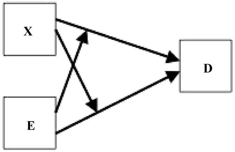
FIGURE 1.

Here the expectation E(D|e,x) is not constant in x for any fixed value of e and is not constant in e for any fixed value of x (ie, they are independent causes of D). Neither E nor X is a cause of the other. However, on the chosen effect modification scale, h(.), for some pair of E values, e₁ and e₀, and some pair of X values, x₁ and x₀, we have effect modification, ie,

$$\begin{array}{c}h[E(D|e_1,x_1)]-h[E(D|e_0,x_0)]\hfill \\ \hfill \ne h[E(D|e_1,x_0)]-h[E(D|e_0,x_0)]+\hfill \\ \hfill h[E(D|e_0,x_1)]-h[E(D|e_0,x_0)]\end{array}$$

Are these classifications helpful? Presumably, the direct and indirect categories of effect modification are the ones with potential implications for intervention, although VanderWeele and Robins do not comment on the utility of their classification scheme.

It has been frustrating to me that important kinds of causal relationships are not captured graphically by DAGs, so I was disappointed that the example DAGs given by VanderWeele and Robins provide no graphical representation to indicate that a factor is regarded as an effect modifier for some other risk factor. Consider their example of a genotype, X, that might influence response to treatment in a randomized clinical trial of an exposure E. Their Figure 1 shows the corresponding DAG. One might have hoped to see causal diagrams that were able to show more interaction than is suggested by the 2 separate, mutually aloof arrows—one from E to D and one from X to D. Perhaps one could instead show an arrow from X that ends at the E-to-D arrow itself, as in my Figure 1. (Refer to the figure legends for how I am defining “direct cause” mathematically.) Note that if both X and E are causes of D, and X is an effect modifier for E, then E is necessarily also an effect modifier for X.

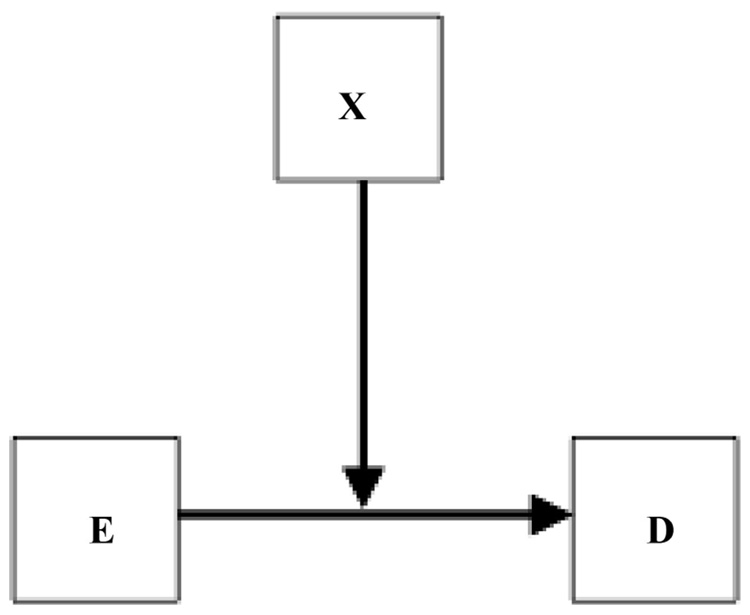
Variations of this causal scenario can also be captured. Consider Figure 1 in VanderWeele and Robins and remove the arrow from X to D. X might influence either the uptake or the metabolism of E, or the biologic response to E, but have no effect on D by itself. Thus, it may only affect the arrow from E to D, ie, the causal process itself. We would not think of X as a “direct cause” of D (its “main effect” would be 0), and we could show this by omitting its direct arrow to D, although the standard DAG might still demand that arrow. In environmental health, some of the most plausible effect modifiers are those that influence absorption, specific metabolic detoxification pathways, immune responses, apoptosis, or DNA repair processes. Some effect-modifying cofactors may have little or no effect in the absence of exposure (although others may retain effects via unmeasured other exposures whose effects are also modified). This phenomenon could be shown graphically as in my Figure 2. Note that this effect modification is present regardless of the scale selected. As another example, the polio vaccine should have no effect on an individual’s risk of developing polio in the absence of exposure to the polio virus.

FIGURE 2.

Here for some value e′ of E, E(D|e′,x) does not vary with x, so X is not an independent risk factor for D. Neither E nor X is a cause of the other. However, on the chosen effect modification scale, h(.), for some pair of E values, e₁ and e₀, and some pair of X values, x₁ and x₀,we have effect modification, ie,

$$\begin{array}{c}h[E(D|e_1,x_1)]-h[E(D|e_0,x_0)]\hfill \\ \hfill \ne h[E(D|e_1,x_0)]-h[E(D|e_0,x_0)]+\hfill \\ \hfill h[E(D|e_0,x_1)]-h[E(D|e_0,x_0)]\end{array}$$

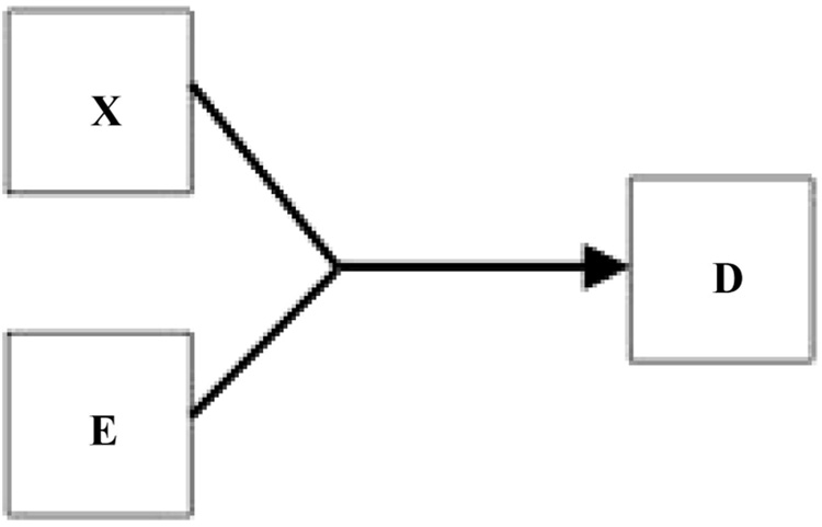
There are also scenarios where both the X-to-D arrow and the E-to-D arrow could be omitted, because neither produces D by itself. This possible category of “pure” effect modification could be represented by arrows that join together, as in my Figure 3. Retardation secondary to phenylketonuria is an example, because neither the genetic metabolic defect nor dietary phenylalanine produces retardation by itself. Note that this kind of scenario also reflects effect modification that is present regardless of the scale selected, and could also be seen as a 2-component, sufficient-cause scenario, as described by Rothman⁴ as a causal pie. More generally, however, I tend to see things in stochastic rather than deterministic terms, and would not expect causal processes that do not involve a highly penetrant mutation to be usefully represented by pies.

FIGURE 3.

Here for some value e′ of E, E(D|e′,x) is constant in x and for some value x′ of X E(D|e,x′) is constant in e, so neither is an independent risk factor for D. Neither E nor X is a cause of the other. However, on the chosen effect modification scale, h(.), for some pair of E values, e₁ and e₀, and some pair of X values, x₁ and x₀, we have effect modification, ie.,

$$\begin{array}{c}h[E(D|e_1,x_1)]-h[E(D|e_0,x_0)]\hfill \\ \hfill \ne h[E(D|e_1,x_0)]-h[E(D|e_0,x_0)]+\hfill \\ \hfill h[E(D|e_0,x_1)]-h[E(D|e_0,x_0)]\end{array}$$

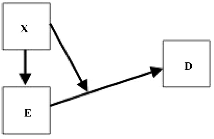
Another kind of scenario that may not be well captured by the usual DAGs is one in which biologic intermediates are included as “E” in the DAG and those intermediates can be phenotypically diverse in ways that have not been identified, but may to some extent depend on how they were caused. Thus, for example, if pesticide exposure in pregnancy causes gestational diabetes,⁵ a known risk factor for developing pre-eclampsia, the condition may sometimes retain a physiologic fingerprint that we have not characterized, but which reflects its causation in a way that has implications for sequelae, eg, the risk of pre-eclampsia. Suppose an exposure X is not causally related to D except through a path involving an intermediate E. Then the risk of D among those with E may still depend on X, as if E retains a memory of its parent, X. This is an interesting kind of effect modification, which could be represented by the graph of Figure 4. Notice that if we did not include the arrow-on-arrow, representing effect modification, we could mistakenly think that D does not depend X once we have conditioned on E. This kind of DAG strongly suggests the existence of diverse subtypes that have been inappropriately lumped into a single intermediate phenotype, subtypes that themselves carry implications for risk. In the example, the phenotypic diversity may be subtle, or may be as simple as variation in severity of gestational diabetes.

FIGURE 4.

Here X is a cause of E, ie, the distribution of E conditional on X = x varies with x. For some value e′ of E, E(D|e′,x) does not vary with x, so X is not an independent risk factor for D. Also, on the chosen effect modification scale, h(.), for some pair of E values, e₁ and e₀, and some pair of X values, x₁ and x₀, we have effect modification, ie,

$$\begin{array}{c}h[E(D|e_1,x_1)]-h[E(D|e_0,x_0)]\hfill \\ \hfill \ne h[E(D|e_1,x_0)]-h[E(D|e_0,x_0)]+\hfill \\ \hfill h[E(D|e_0,x_1)]-h[E(D|e_0,x_0)]\end{array}$$

Having proposed Figure 1 to Figure 4, which seem to me to capture more about effect modification than do the usual DAGs, there may be some formal logic reason to avoid arrow-intersecting graphs; such graphs are probably not kosher within formal directed acyclic graph theory. It may also be that, once one allows arrow-on-arrow effects and begins to think about representing overlapping sets of contributing causes, the resulting tangle of arrows begins to look too much like some kind of pasta, and the complexity may become daunting.

I consider the terminology itself to be a significant problem in thinking about models for joint effects: “effect modification” may be the most unfortunate jargon in epidemiology. The phrase strongly implies that a cofactor actually is acting to modify the causal effect we are studying, and investigators (and others) can be seduced by the words into presuming their finding has causal meaning. In practice, a finding of “interaction” or “effect modification” usually means little more than inequality of an estimated parameter across strata, which is a much more accurate but less sexy way to say the same thing.

VanderWeele and Robins³ step very carefully around the old issues related to the choice of scale one should use when defining and identifying effect modification. Readers who favor an additive model, because it is of more immediate public health relevance than the popular multiplicative model, will appreciate their choice of the risk-difference scale in which to assess effect modification. Although they develop their ideas in a context where effect modification is based on a risk-difference criterion, VanderWeele and Robins point out that one could alternatively use either the risk ratio (log risk) or the odds ratio (log odds) as the scale for defining effect modification. The richness of these choices for identifying “effect modifiers” becomes clear if one considers the fact that if E is a risk factor, then any second risk factor must be an “effect modifier” for the effect of E on at least 2 of those 3 scales. Basic algebra guarantees that effect modification is all around us, while all this plenty must also make some of us doubt its usefulness as a statistical and epidemiological construct.

Nonetheless, a scale I think should be more often considered because it may sometimes actually have causal meaning, but one not mentioned by VanderWeele and Robins, is the log-complement scale. This is the scale that attempts to capture probabilistic independence among causal processes. Toxicologists developed the concept of “simple independent action” for toxic effects of 2 different chemicals administered simultaneously.⁶ The idea, which has also been discussed in the context of epidemiology,⁷ is simple. Suppose that exposure A can cause D and exposure B can cause D by a truly independent pathway, while D can also occur in the absence of either A and B through an independent background cause. The paradigm would be 2 hunters who are independently aiming at the same duck. Of course, the duck could also drop dead from some unrelated and independent background cause, eg, lightning. If the 3 pathways are probabilistically independent, we have:

$$\begin{array}{c}\text{Pr}[\overline{D}|A,\overline{B}]=\hfill \\ \text{Pr}[\text{avoid casual effect of background}]\text{Pr}[\text{avoid casual effect of A}];\hfill \\ \text{Pr}[\overline{D}|\overline{A},B]=\hfill \\ \text{Pr}[\text{avoid causal effect of background}]\text{Pr}[\text{avoid causal effect of B}];\\ \text{and}\text{Pr}[\overline{D}|A,B]=\text{Pr}[\overline{D}|A,\overline{B}]\text{Pr}[\text{avoid casual effect of B}].\hfill \end{array}$$

Hence we have that:

$$\text{Pr}[\overline{D}|A,B]=\frac{\text{Pr}[\overline{D}|A,\overline{B}]\text{Pr}[\overline{D}|\overline{A},B]}{\text{Pr}[\overline{D}|\overline{A},\overline{B}]}.$$

Under probabilistically independent effects then, it follows that there is additivity on the log complement scale:

$$\frac{\text{Pr}[\overline{D}|A,B]\text{Pr}[\overline{D}|\overline{A},\overline{B}]}{\text{Pr}[\overline{D}|A,\overline{B}]\text{Pr}[\overline{D}|\overline{A},B]}=1;$$

that is,

$$\begin{array}{c}\text{ln}(\text{Pr}[\overline{D}|A,B])-\text{ln}(\text{Pr}[\overline{D}|\overline{A},\overline{B}])\hfill \\ \hfill =[\text{ln}(\text{Pr}[\overline{D}|A,\overline{B})-\text{ln}(\text{Pr}[\overline{D}|\overline{A},\overline{B}]+\hfill \\ \hfill [\text{ln}(\text{Pr}[\overline{D}|\overline{A},B])-\mathit{\text{ln}}(\mathit{\text{Pr}}[\overline{D}|\overline{A},\overline{B}])]\end{array}$$

Thus there is additivity of the effect of A and the effect of B, on the log-complement scale. For a rare outcome, the analogous additive model will approximately hold on the absolute risk scale. However, when the outcome is not rare, additivity of risks is not equivalent to statistical independence (there being a non-negligible chance that both hunters will hit the duck), so is not equivalent to additivity on the log complement scale.

When we study more than one individual, variation across individuals in susceptibility (certain ducks may be easier for the independently shooting hunters to see) can cause violations of probabilistic independence, even if stochastic independence of causes holds for each individual at risk, so even this (to me) appealing formulation does not necessarily permit a biologically meaningful inference.⁷ Moreover, one must also think differently and in a more complicated way about protective factors, such as vaccines. Nonetheless, although the field may have grown weary of this debate, issues of scale will continue to matter when we try to draw useful inference from models for joint effects.

DAGs have met with a mixed reaction in epidemiology, with some of my colleagues recognizing their importance for analysis of etiologic factors, and others preferring to think about confounding in more classic terms. I have long been one of the boosters.

One practical challenge with DAGs in my experience, however, is the contentiousness of choosing a DAG. These choices can be especially problematic in reproductive epidemiology, where time-related factors become important. For example: Is long interpregnancy interval a cause of change of partner, or is change of partner a cause of long interpregnancy interval? But the hard thinking and very careful consideration of the etiologic context that are needed to decide which DAG is epidemiologically most plausible can be extremely useful, as we try to break through our academically enforced reluctance to think directly about causes.

A different, longstanding problem with DAGs has been that when synergistic effects may be involved in the etiology of the disease, DAGs are annoyingly noncommittal. I’m afraid the paper by VanderWeele and Robins,³ although providing useful categorizations for effect modifiers, has not rescued DAGs from this limitation. There may be more future in rethinking the basics of how we draw the DAGs.

REFERENCES

- 1.Pearl J. Probabilistic Reasoning in Intelligent Systems: Networks of Plausible Inference. Burlington, MA: Morgan Kaufmann; 1988. [Google Scholar]
- 2.Greenland S, Pearl J, Robins J. Causal diagrams for epidemiologic research. Epidemiology. 1999;10:37–48. [PubMed] [Google Scholar]
- 3.VanderWeele TJ, Robins JM. Four types of effect modification—a classification based on directed acyclic graphs. Epidemiology. 2007;18:561–568. doi: 10.1097/EDE.0b013e318127181b. [DOI] [PubMed] [Google Scholar]
- 4.Rothman K, Greenland S. Modern Epidemiology. 2nd ed. Philadelphia: Lippincott-Raven Publishers; 1998. [Google Scholar]
- 5.Saldana TM, Basso O, Hoppin JA, et al. Pesticide exposure and self-reported gestational diabetes mellitus in the Agricultural Health Study. Diabetes Care. 2007;30:529–534. doi: 10.2337/dc06-1832. [DOI] [PMC free article] [PubMed] [Google Scholar]
- 6.Bliss CI. The toxicity of poisons applied jointly. Ann Appl Biol. 1939;26:585–615. [Google Scholar]
- 7.Weinberg CR. Applicability of the simple independent action model to epidemiologic studies involving two factors and a dichotomous outcome. Am J Epidemiol. 1986;123:162–173. doi: 10.1093/oxfordjournals.aje.a114211. [DOI] [PubMed] [Google Scholar]