The properties of high-dimensional data spaces: implications for exploring gene and protein expression data

Abstract

High-throughput genomic and proteomic technologies are widely used in cancer research to build better predictive models of diagnosis, prognosis and therapy, to identify and characterize key signalling networks and to find new targets for drug development. These technologies present investigators with the task of extracting meaningful statistical and biological information from high-dimensional data spaces, wherein each sample is defined by hundreds or thousands of measurements, usually concurrently obtained. The properties of high dimensionality are often poorly understood or overlooked in data modelling and analysis. From the perspective of translational science, this Review discusses the properties of high-dimensional data spaces that arise in genomic and proteomic studies and the challenges they can pose for data analysis and interpretation.

Genomic microarray and proteomic technologies provide powerful methods with which systems biology can be used to address important issues in cancer biology. These technologies are often used to identify genes and proteins that may have a functional role in specific phenotypes. It is becoming possible to define expression patterns that can identify specific phenotypes (diagnosis)^1,2, establish a patient’s expected clinical outcome independent of treatment (prognosis)^3,4 and predict a potential outcome from the effects of a specific therapy (prediction)^5,6 (BOX 1). One recent example is the MammaPrint prognostic gene-expression signature, the first multivariate in vitro diagnostic assay approved for use by the US Food and Drug Administration. The gene set is based on the Amsterdam 70-Gene Profile, derived from the analysis of 25,000 human genes in a series of 98 primary breast cancers⁷. Subsequently, the signature (or classifier) was verified in an independent series of 295 breast cancers⁸. Activity levels of the genes in the signature are translated into a score that is used to classify patients into those at high risk and those at low risk of recurrent disease, thereby informing decisions on treatment strategy to deliver appropriate treatment according to each patient’s risk classification⁷. MammaPrint is applicable for patients diagnosed with node-negative, stage I or stage II breast cancer, demonstrating a place for molecular-based technologies in modern medicine.

Box 1 Genomic and proteomic technologies used in cancer research.

Many systems-biology technologies that are used to address questions in cancer research, such as biomarker selection, cancer classification, cell signalling and predicting drug responsiveness, generate high-dimensional data. Among the more common technologies used are gene expression microarrays, serial analysis of gene expression^21,94, two-dimensional differential gel electrophoresis^95,96, protein chips¹⁰ and antibody-based arrays⁹⁷. The high dimensionality of the data is readily illustrated; the U133 Plus 2 whole human genome expression array (Affymetrix) can probe for the expression of 47,000 transcripts in a single sample. Similar numbers of measurements are obtained in proteomic analysis, such as those using the ProteinChip System (Ciphergen)¹⁰. Although we are primarily discussing transcriptome and proteome profiling, high-throughput screening for genetic changes in DNA by comparative genomic hybridization (array CGH) can also generate high-dimensional data^98,99. High-throughput single nucleotide polymorphism analysis (SNP-chips¹⁰⁰), promoter analysis such as screening methylation status (methylation chips)¹⁰¹ or genome-wide location analysis (chromatin immunoprecipitation-on-chip)¹⁰² are also now being used and can generate multiple measurements on a single sample.

The data are high-dimensional because 100s–1,000s of individual measurements are obtained on each specimen. As shown in the table, there are unique challenges associated with these data. These challenges include knowing that the statistical solution is correct, complete or accurate and avoiding the trap of self-fulfilling prophesy. Assessing the accuracy of the statistical solution is of particular concern when the data are subject to the curse of dimensionality, or when the data are either unsupervised or where the supervising information is inadequate. Using incomplete biological knowledge to guide class identification can lead to incorrect class assignment or incorrect data interpretation. Avoiding the trap of self-fulfilling prophesy is a challenge for which incomplete knowledge of gene function and cellular context can lead to the creation of incorrect signalling links in network building. For all classification studies, including those directed at prediction or prognosis, validation in independent data sets is essential. For cell signalling and mechanistic studies, independent functional validation of linkages and signalling is essential (studies in cell cultures, animal models, gene transfection, small interfering RNA and so on).

Research question	High-dimensional problems
Biomarker selection (find individual genes or groups of genes that are functionally relevant and/or surrogates for a specific clinical outcome).	Trade-off between accuracy and computational complexity; confound of multimodality; spurious correlations; multiple testing; insufficient sensitivity of criterion function; curse of dimensionality; model overfitting.
Cancer classification (find new molecular subclasses within a cancer that exhibit meaningful clinical or biological properties, for example, that enable physicians to better direct treatment).	Curse of dimensionality; confound of multimodality; spurious clusters; model overfitting; small sample size; biased performance estimate.
Cancer prognosis (predict which patients will have a particularly good or poor outcome and enable physicians to better direct treatment).	Curse of dimensionality; confound of multimodality; spurious correlations; model overfitting; small sample size; biased performance estimate.
Cell signaling (identify how cell signalling affects cancer cell functions and identify new targets for drug development).	Curse of dimensionality; confound of multimodality; spurious correlations; multiple testing.
Predicting drug responsiveness (identify genes or patterns of genes that will predict how a cancer will respond to a specific therapeutic strategy and enable physicians to better direct treatment).	Curse of dimensionality; confound of multimodality; spurious correlations; model overfitting; small sample size.

Despite the encouraging progress of the MammaPrint classifier, the application of modern systems-biology techniques has introduced into cancer research the problems of working in high-dimensional data spaces, wherein each sample can be defined by hundreds or thousands of measurements. Gene microarray analysis of a single cancer specimen could yield concurrent measurements on >10,000 detectable mRNA transcripts. Even after a simple pair-wise analysis to select differentially expressed genes in a supervised analysis (see discussion of supervised analysis below), for example, using t-test or false discovery rate (FDR) methodology, the data structure may still contain information on >1,500 genes per sample in a study with a small sample size⁹ (BOX 2). Dimensionality may be much larger in proteomic studies¹⁰. Although often encountered in other fields, such as engineering and computer science, this data structure is unlike most others in biomedicine. Our goal in this Review is not to provide a guide to data analysis, as this has been done by others^11,12. Rather, we discuss the theory and properties of these data spaces and highlight how they may affect data analysis and interpretation. We also describe the basic properties of high-dimensional data structures and discuss the challenges these pose for extracting accurate, reliable and optimal knowledge.

Box 2 Multiple testing in high dimensions.

A common goal in genomic and proteomic studies is to find informative and discriminant genes (genes for which their values distinguish or discriminate between two (or more) groups, such as selecting biomarkers in BOX 1). Typically, investigators face the problem of testing the null hypothesis for thousands of genes simultaneously. If we only use the type I error α = 0.05 for each gene the possible number of type I errors (false positive; identifying a gene’s expression as being different between groups when it is not) is large because we are conducting thousands of tests simultaneously:

Number of type I errors = number of comparisons × α

For example, for n = 10,000 genes and α = 0.05 there are 500 potential type I errors.

Assuming that genes are independently expressed, the experiment-wide α for n independent comparisons is as shown:

α_{experiment-wide} = 1−(1−α_{per independent comparison})ⁿ

For example, with 10 independent comparisons and α_{per independent comparison} = 0.05, the estimated α_{experiment-wide} is already 0.40 (a probability of 1.0 would be a guarantee of an error).

Most approaches to address the multiple-testing problem are too conservative¹⁰³ and over-constrain the type I error and inflate the type II error (β; false negatives). For classification problems, for example, predicting cancer recurrence, this limitation may be acceptable because we are not interested in gene function, only in the ability to separate the classes. Family-wise error rate and false-discovery rate approaches have been widely used to control the probability of one or more false rejections and the expectation of the proportion of false-positive errors, respectively¹⁰⁴; several other approaches also have shown usefulness^24,105. However, the multiple-testing problem is particularly challenging for signalling pathway studies because the statistical properties of a gene’s signal are not direct measures of its biological activity. False negatives are rarely considered but may include mechanistically relevant genes. An estimate of the miss rate provides one approach to guide exploration of the potential false negatives¹⁰⁶.

A central problem with many univariate and multivariate methods is the assumption of independence — that the expression of each gene is independent of all others — but all genes do not function independently. The extent and nature of correlated events may violate the assumptions of various statistical models, whether or not the multiple-comparisons problem is adequately controlled. Methods to deal with these issues continue to appear in the biomedical literature^107-109. Functional validation of these methods on multiple data sets is required, as is compelling evidence that new methods are both theoretically sound and outperform existing methods.

We consider data structure from several perspectives. In the simplest sense, these data represent a direct or indirect assessment of the levels of expression of 100s to 10,000s of mRNA transcripts or proteins. These values reside in space characterized by multiple additional properties, as the space is also defined by the biological properties of the specimens from which they were obtained, by the functional interactions among co-expressed genes or proteins in signalling networks, and by the experimental design. Each of these factors can affect data structure and the ability to analyse it effectively. We begin by discussing key aspects of data spaces that affect many experimental designs. We then describe the properties of high-dimensional data spaces and how they affect the derivation of meaningful information from the data.

At a glance.

• The application of several high-throughput genomic and proteomic technologies to address questions in cancer diagnosis, prognosis and prediction generate high-dimensional data sets.

• The multimodality of high-dimensional cancer data, for example, as a consequence of the heterogeneous and dynamic nature of cancer tissues, the concurrent expression of multiple biological processes and the diverse and often tissue-specific activities of single genes, can confound both simple mechanistic interpretations of cancer biology and the generation of complete or accurate gene signal transduction pathways or networks.

• The mathematical and statistical properties of high-dimensional data spaces are often poorly understood or inadequately considered. This can be particularly challenging for the common scenario where the number of data points obtained for each specimen greatly exceed the number of specimens.

• Data are rarely randomly distributed in high-dimensions and are highly correlated, often with spurious correlations.

• The distances between a data point and its nearest and farthest neighbours can become equidistant in high dimensions, potentially compromising the accuracy of some distance-based analysis tools.

• Owing to the ‘curse of dimensionality’ phenomenon and its negative impact on generalization performance, for example, estimation instability, model overfitting and local convergence, the large estimation error from complex statistical models can easily compromise the prediction advantage provided by their greater representation power. Conversely, simpler statistical models may produce more reproducible predictions but their predictions may not always be adequate.

• Some machine learning methods address the ‘curse of dimensionality’ in high-dimensional data analysis through feature selection and dimensionality reduction, leading to better data visualization and improved classification.

• It is important to ensure that the generalization capability of classifiers derived by supervised learning methods from high-dimensional data before using them for cancer diagnosis, prognosis or prediction. Although this can be assessed initially through cross-validation methods, a more rigorous approach is needed, that is, to validate classifier performance using a blind validation data set(s) that was not used during supervised learning.

Basic transcriptome or proteome data structure

Data points can be seen from the perspective of either the samples or the individual genes or proteins. Viewed from the perspective of the samples, each sample exists in the number of dimensions defined by the number of gene or protein signals that are measured. This is a common perspective in cancer classification, patient survival analysis, identification of significantly expressed genes and other studies in which patients or samples are treated as observations and genes or proteins are treated as variables. These data structures are the primary focus of this Review. By contrast, studies in which genes or proteins are treated as observations and samples or patients are treated as variables, such as in gene function prediction^13,14, face low-dimensional challenges because there may be insufficient observations (genes or proteins) in specific gene function classes for a supervised classification.

Transcriptome and proteome data comprise a mixture of discrete categories (clusters), each category defining a specific class. Clusters are subgroups of data that are more like each other than like any other subgroup of data, and are scattered throughout high-dimensional data spaces (FIG. 1a,b). Each class can be defined by the goal of the experiment, which might be a phenotype (such as recurrent or non-recurrent), a response (responder or non-responder), a treatment (treated, untreated or specific dose), a timed event (time points in a longitudinal study) or some other measure. A class can be represented by more than one cluster. Expression data are massively parallel (FIG. 2) and represent a snapshot of the state of the transcriptome or proteome at the time the specimen was collected. However, some biological functions proceed in a stepwise fashion and these may be inadequately captured in a snapshot. Regulation of expression of some genes is multifactorial, with the key regulatory determinants differing among cell and tissue types and, indeed, among individuals. Some genes can perform different functions in different cells, and different genes can perform more or less the same function in the same cell¹⁵. Hence, the activity of some genes is cell context-dependent; the cellular context is defined by the patterns of gene or protein expression and activation within a cell¹⁶. This biological complexity, where function can be influenced by concurrent, sequential, redundant, degenerate, interdependent or independent events¹⁵, complicates the ability to fully discover the information contained within high-dimensional data.

Figure 1. Cluster separability in data space.

a | Each data point exists in the space defined by its attributes and by its relative distance to all other data points. The nearest neighbour (dashed arrow) is the closest data point. The goal of clustering algorithms is to assign the data point to membership in the most appropriate cluster (red or blue cluster). Many widely used analysis methods force samples to belong to a single group or link them to their estimated nearest neighbour and do not allow concurrent membership of more than one area of data space (hard clustering; such as k-means clustering or hierarchical clustering based on a distance matrix). Analysis methods that allow samples to belong to more than one cluster (soft clustering; such as that using the expectation-maximization algorithm) may reveal additional information. b | Data classes can be linearly separable or non-linearly separable. When linearly separable, a linear plane can be found that separates the data clusters (i). Non-linearly separable data can exist in relatively simple (ii) or complex (iii) data space. Well-defined clusters in simple data space may be separated by a non-linear plane (ii). In complex data space, cluster separability may not be apparent in low-dimensional visualizations (iii), but may exist in higher dimensions (iv). c | Expression data can be represented as collections of continuously valued vectors, each corresponding to a sample’s gene-expression profile. Data are often arranged in a matrix of N rows (samples) and D columns (variables or genes). The distance of a data point to the origin (vector space), or the distance between two data points (metric space), is defined by general mathematical rules. A (blue arrow) and B (green arrow) are vectors and their Euclidean distance is indicated by the red line. Individual data points, each represented by a vector, can form clusters, as in the examples of two clusters in b.

Figure 2. High dimensional expression data are multimodal.

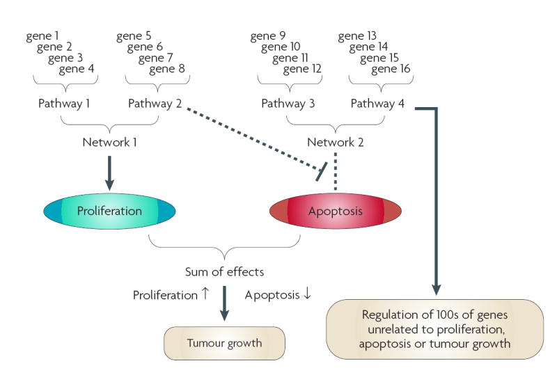
Most univariate and multivariate probability theories were derived for data space where N (number of samples) > D (number of dimensions). Expression data are usually very different (D>>>N). A study of 100 mRNA populations (one from each of 100 tumours) arrayed against 10,000 genes can be viewed as each of the 100 tumours existing in 10,000-D space. This data structure is the inverse of an epidemiological study of 10,000 subjects (samples) for which there are data from 100 measurements (dimensions), yet both data sets contain 10⁶ data points. A further concern arises from the multimodal nature of high-dimensional data spaces. The dynamic nature of cancer and the concurrent activity of multiple biological processes occurring within the microenvironment of a tumour create a multimodal data set. Genes combine into pathways; pathways combine into networks. Genes, pathways and/or networks interact to affect subphenotypes (proliferation, apoptosis); subphenotypes contribute to clinically relevant observations (tumour size, proliferation rate). Genes in pathway 2 are directly associated with a network (and with pathway 1) and a common subphenotype (increased proliferation). Genes in pathway 2 are also inversely associated with a subphenotype (apoptosis). Here, multimodality captures the complex redundancy and degeneracy of biological systems¹⁵ and the concurrent expression of multiple components of a complex phenotype. For example, tumour growth reflects the balance between cell survival, proliferation and death, and cell loss from the tumour (such as through invasion and metastasis), each being regulated by a series of cellular signals and functions. Many such complex functions may coexist, such as growth-factor or hormonal stimulation of tumour cell survival or proliferation, or the ability to regulate a specific cell-death cascade. A molecular profile from a tumour may contain subpatterns of genes that reflect each of these individual characteristics. This multimodality may be problematic for statistical modelling to build either accurate cell signalling networks or robust classification schemes.

Most common approaches to exploring entire expression profiles use some measure of distance within Euclidean space (mathematical geometric model) as a means to establish the relationship among data points (FIG. 1c). For example, the numerator in a t-test equation uses the Euclidean distance between the means of the two populations. A k-means clustering algorithm uses various Euclidean distances to measure the distance from a data point to the estimated median of a cluster. A support vector machine (SVM; BOX 3) measures the distance of a data point or pattern from the boundary between the two populations in Euclidean space. A common method is hard clustering using a Pearson correlation matrix to construct a hierarchical representation of the data¹⁷, used, for example, to discover five new molecular subclasses of breast cancer¹⁸. The k-nearest neighbour (kNN) decision rule assigns similar patterns to the same class and requires computation of the distance between a test pattern and all the patterns in the training set¹⁹. The number of neighbourhoods, k, is set by the user. If k = 1, the test pattern is then assigned to the class of the closest training pattern¹⁹. For k = 3, 5, 7… the majority vote is applied based on the assumption that the characteristics of members of the same class are similar. A kNN approach was used in a recent study to define molecular subclasses of childhood acute leukaemias²⁰.

Box 3 Support vector machines.

The support vector machine (SVM) is a powerful Binary classifier rooted in statistical learning theory¹¹⁰. It can theoretically achieve a global optimum solution (convex optimization) and bypass the curse of dimensionality³⁶. The SVM provides a way to control model complexity independent of dimensionality and offers the possibility to construct generalized, non-linear predictors in high-dimensional spaces using a small training set¹⁹.

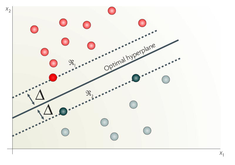
Training an SVM involves finding the optimal separating hyperplane that has the maximum distance from the nearest training patterns (see figure: the optimal hyperplane separates the patterns into regions ℛ₁ (red patterns) and ℛ₂ (grey patterns). The support vectors (shown in the figure as a dark red dot in region ℛ₁ and dark grey dots in region ℛ₂) define the optimal hyperplane^19,36,111. As the nearest training patterns to the optimal hyperplane, support vectors are the most informative patterns for classification¹¹². Once the optimal hyperplane is determined, it serves as a decision boundary to classify an unknown pattern into one of the two regions.

The example in the figure presents patterns from two classes in two linearly separable regions (ℛ₁ and ℛ₂). In complex classification problems, where the patterns are distributed in two linearly inseparable classes, SVM uses non-linear kernel functions to implicitly map the patterns to a higher-dimensional feature space³⁶. Then, the optimal hyperplane is determined to maximize the margin of separation between the two classes in the feature space.

The original SVM was designed for binary classification. Many classification tasks involve more than two classes and the most common multi-category SVMs use a ‘one-versus-all approach’¹¹³. A SVM is built for each category by comparing it against all others; for k-category classification, k binary SVM classifiers are built: category 1 versus all others, category 2 versus all others and so on up to category k versus all others¹¹³. To classify an unknown sample, the distance from the sample to each classifier’s hyperplane is calculated and the sample is classified into the category with the farthest positive hyperplane. In terms of traditional template-matching techniques, support vectors replace the prototypes for which characterization is not just defined by the minimum distance function, but by a more general and possibly non-linear combination of these distances⁹⁰. SVMs are not applicable to all data sets and mining tasks. The ad hoc character of the penalty terms (error penalty) and the computational complexity of the training procedure are limitations. SVMs are sensitive to mislabelled training samples and they are not fully immune to the curse of dimensionality¹¹¹.

Supervised and unsupervised analyses

Among the most common experimental designs are those aimed at finding molecular profiles that establish a patient’s prognosis, or identify those signalling events that drive a specific biological property of a cancer cell line, mouse model, therapy or other manipulation (for examples, see REFS ^6,21,22). Studies in which the endpoint measurements that are associated with the respective expression pattern(s) are known (that is, there is external information that can be used to guide and evaluate the process) are termed supervised analyses; these generally have the greatest power to correctly identify important molecular changes. For example, when one group of samples (class 1: sensitive to a cytotoxic drug) is compared with another (class 2: resistant to a cytotoxic drug), the external knowledge is the class membership of the samples under analysis. The analysis can proceed to find genes or proteins that are differentially expressed between the two classes. These genetic or proteomic profiles can then be used to build a classifier to predict whether unknown samples belong to class 1 or class 2; that is, the classifier is trained on a series of samples for which class membership is known and then validated on an independent data set. An independent data set is one for which class membership is known but the data are not from the samples used to identify the profile or train the classifier. This approach allows the accuracy of the classifier to be determined without the outcome being biased by using the same input data used to build or train the predictor (FIG. 3). Supervised analysis can be used for many aspects of high-dimensional data analysis, including dimensionality reduction, feature selection and predictive classification.

Figure 3. Model fitting, dimensionality and the blessings of smoothness.

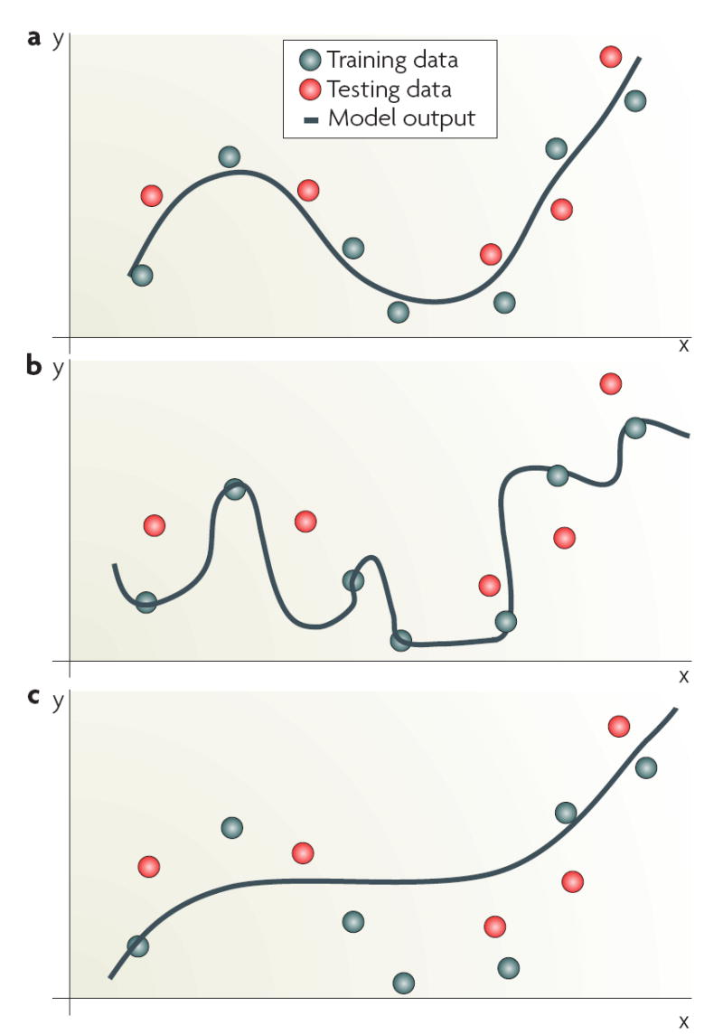
a | Output of a smooth function that yields good generalization on previously unseen inputs. b | A model that performs well on the training data used for model building, but fails to generalize on independent data and is hence overfitted to the training data. c | A model that is insufficiently constructed and trained and is considered to be underfitted. The imposition of stability on the solution can reduce overfitting by ensuring that the function is smooth, and some random fluctuations are well-controlled in high-dimensions⁴⁶. This allows new samples that are similar to those in the training set to be similarly labelled. This phenomenon is often referred to as the ‘blessing of smoothness’. Stability can also be imposed using regularization that ensures smoothness by constraining the magnitude of the parameters of the model. Support vector machines apply a regularization term that controls the model complexity and makes it less likely to overfit the data (BOX 3). By contrast, k-nearest neighbour or weighted voting average algorithms overcome the challenge simply by reducing data dimensionality. Validation of performance is a crucial component in model building. Although an iterative sequential training is often used for both training and optimization¹¹⁴, validation must be done using an independent data set (not used for model training or optimization) and where there are adequate outcomes relative to the number of variables in the model³⁹. For early proof-of-principle studies, for which an independent data set may not be available, some form of cross-validation can be used. For example, three-fold cross-validation is common, in which the classifier is trained on two-thirds of the overall data set and tested for predictive power on the other third³⁶,¹¹⁵,¹¹⁶. This process is repeated multiple times by reshuffling the data and re-testing the classification error.

Unsupervised cluster analyses are an important tool for discovering underlying cancer subtypes or gene modules^23,24 and can also be applied when information for supervised analyses is available to suggest refinements of known cancer categories: categorical labels are purposely withheld or used to initiate a clustering algorithm²⁵ (FIG. 1). Class labels can subsequently be used to validate the clustering methodology and assumptions, where strong correlations among clustering outcomes and known class labels support the applicability of this clustering approach to other unlabelled microarray data²³. The study by Golub et al.²³ of acute myeloid leukaemia and acute lymphoblastic leukaemia is one example of the use of unsupervised analysis on data from samples with known histopathological subtypes (supervised data).

Applying unsupervised methods to data with known categorical information might seem counterintuitive. However, an important consideration is the quality of the known categorical information, as the extent to which data membership is defined by existing information might be incomplete. Consider a study of the anthracycline anticancer drug doxorubicin with two goals: the first to identify the mechanism of doxorubicin action and resistance, and the second to build a clinically meaningful predictor of doxorubicin responsiveness. For the first goal (molecular signalling), a common assumption is that all tumours will respond to doxorubicin in the same way. However, data may not be fully defined by the binary outcomes (supervision) of sensitivity and resistance. For example, doxorubicin can both produce chemically reactive metabolites that damage nucleic acids and proteins (mechanism 1) and inhibit topoisomerase II, an enzyme involved in maintaining DNA topology (mechanism 2)^26,27. If doxorubicin can kill cells through either mechanism, some tumours may be more sensitive to one mechanism than to the other. If only one responsive phenotype is assumed but both occur, a supervised analysis comparing all sensitive with all resistant tumours could fail to identify, either correctly and/or completely, consistent changes in gene expression that would identify either pathway.

An effective unsupervised analysis might allow the discovery of several molecular signatures associated with doxorubicin responsiveness. Information that defines outcome (sensitive versus resistant) could be used to assess the accuracy of the unsupervised clustering solution. Some of the clusters found might contain a high proportion of doxorubicin-sensitive tumours (clusters representing sensitivity to mechanisms 1, 2 and/or unknown mechanisms) whereas other clusters may contain mostly resistant tumours (resistant to mechanisms 1, 2 and/or unknown mechanisms).

To construct a classifier of prediction in a supervised analysis, the supervising information may be a measure of clinical response used as a surrogate for a long-term outcome such as survival. The choice of surrogate endpoint then becomes a crucial component of how to define and test a classifier of responsiveness. If the study applies a neoadjuvant design, the surrogate of palpable tumour shrinkage (clinical response) may be suboptimal compared with pathological response. A complete pathological response is usually a better predictor of survival outcome because microscopic disease rather than tumour shrinkage is evaluated^28-30. When the pathological data are not available, an unsupervised method may help find those complete clinical responses that are not true complete pathological responses: hence, two subclusters might be identified within the group defined as complete clinical responses. These simple examples emphasize the importance of the hypothesis and the experimental design, and how these can affect the approach to data analysis.

Properties of high-dimensional data spaces

The properties of high-dimensional data can affect the ability of statistical models to extract meaningful information. For genomic and proteomic studies, these properties reflect both the statistical and mathematical properties of high-dimensional data spaces and the consequences of the measured values arising from the complexity of cancer biology. This section discusses such issues and their implications.

The curse of dimensionality

The performance of a statistical model depends on the interrelationship among sample size, data dimensionality, model complexity¹⁹ and the variability of outcome measures. Optimal model fitting using statistical learning techniques breaks down in high dimensions, a phenomenon called the ‘curse of dimensionality’³¹. FIGURE 4 illustrates the effects of dimensionality on the geometric distribution of data and introduces the performance behaviour of statistical models that concurrently use a large number of input variables. For example, a naive learning technique (dividing the attribute space into cells and associating a class label with each cell) requires the number of training data points to be an exponential function of the attribute dimension¹⁹. Thus, the ability of an algorithm to converge to a true model degrades rapidly as data dimensionality increases³².

Figure 4. The curse of dimensionality and the bias or variance dilemma.

a | The geometric distributions of data points in low- and high-dimensional space differ significantly. For example, using a subcubical neighbourhood in a 3-dimensional data space (red cube) to capture 1% of the data to learn a local model requires coverage of 22% of the range of each dimension (0.01 ≈ 0.22³) as compared with only 10% coverage in a 2-dimensional data space (green square) (0.01 = 0.10²). Accordingly, using a hypercubical neighbourhood in a 10-dimensional data space to capture 1% of the data to learn a local model requires coverage of as much as 63% of the range of each dimension (0.01 ≈ 0.63¹⁰). Such neighbourhoods are no longer ‘local’¹¹¹. As a result, the sparse sampling in high dimensions creates the empty space phenomenon: most data points are closer to the surface of the sample space than to any other data point¹¹¹. For example, with 5,000 data points uniformly distributed in a 10-dimensional unit ball centred at the origin, the median distance from the origin to the nearest data point is approximately 0.52 (more than halfway to the boundary), that is, a nearest-neighbour estimate at the origin must be extrapolated or interpolated from neighbouring sample points that are effectively far away from the origin¹¹¹. b | A practical demonstration is the bias–variance dilemma³⁶,¹¹¹,¹¹⁵. Specifically, the mismatch between a model and data can be decomposed into two components; bias that represents the approximation error, and variance that represents the estimation error. Added dimensions can degrade the performance of a model if the number of training samples is small relative to the number of dimensions. For a fixed sample size, as the number of dimensions is increased there is a corresponding increase in model complexity (increase in the number of unknown parameters), and a decrease in the reliability of the parameter estimates. Consequently, in the high-dimensional data space there is a trade-off between the decreased predictor bias and the increased prediction uncertainty³⁶,¹¹¹.

The application of statistical pattern recognition to molecular profiling data is complicated by the distortion of data structure. For many neural network classifiers, learning is confounded by the input of high-dimensional data and the consequent large search radius — the network must allocate its resources to represent many irrelevant components of this input space (data attributes that do not contribute to the solution of data structure). When confronted with an input of 1,500 dimensions (D), much of the data space will probably contain irrelevant data subspaces unevenly distributed within the data space³³. Supervised or unsupervised algorithms can fail when attempting to find the true relationships among individual data points for each sample and among different groups of similar data³². Thus, the data solution obtained may be incorrect, incomplete or suboptimal.

Because of the high dimensionality of the input data, arriving at an adequate or correct solution will generally be computationally intensive. Although simple models, such as some hierarchical clustering approaches, may not be computationally affected, these are often inappropriate for tasks other than visualization^11,34. Simple models can perform well when the structure of the data is relatively simple, for example, a small number of well-defined clusters³⁵, but may be less effective for complex data sets. A further challenge for modelling is to avoid overfitting the training data (FIG. 3b). Clearly, it is necessary to have methods that can produce models with good generalization capability. Models derived from a training data set are expected to apply equally well to an independent data set. FIGURE 3 illustrates the effects of overfitting and underfitting and the need for smoothness regularization in a curve-fitting problem³⁶.

The often small number of sample replicates further compounds the problems of multimodal, high-dimensional data spaces. The number of replicate estimates of each sample is usually limited; often only a single measurement is obtained³⁷. Moreover, the number of data features may be so large that an adequate number of samples cannot be obtained for accurate analysis. For example, logistic regression modelling is widely used to relate one or more explanatory variables (such as a cancer biomarker) to a dependent outcome (such as recurrence status) with a binomial distribution. However, the ability to model high-dimensional data accurately and robustly is restricted by the ‘rule of 10’ (REF. ³⁸); Peduzzi et al.³⁹ showed that regression coefficients can be biased in both directions (positive and negative) when the number of events per variable falls below 10. For example, a logistic regression model relating the expression of 50 genes (variables) to a binary clinical outcome such as doxorubicin responsiveness, for which the response rate was approximately 25%, might require a study population of 2,000 to obtain 500 responders (10 times the number of genes as required by the rule of 10 and 25% of the study population) and 1,500 non-responders.

Two of the more common approaches to addressing the properties of high dimensionality are reducing the dimensionality of the data set (FIG. 5) or applying or adapting methods that are independent of data dimensionality. For classification schemes, SvMs are specifically designed to operate in high-dimensional spaces and are less subject to the curse of dimensionality than other classifiers (BOX 3).

Figure 5. Dimensionality reduction.

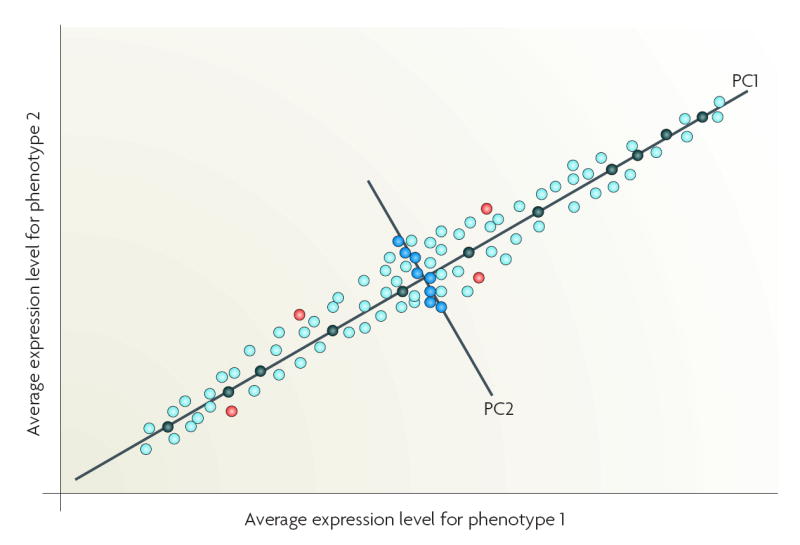
A practical implication of the curse of dimensionality is that, when confronted with a limited training sample, an investigator will select a small number of informative features (variables or genes). A supervised method can select these features (reduce dimensionality), where the most useful subset of features (genes or proteins) is selected on the basis of the classification performance of the features. The crucial issue is the choice of a criterion function. Commonly used criteria are the classification error and joint likelihood of a gene subset, but such criteria cannot be reliably estimated when data dimensionality is high. One strategy is to apply bootstrap re-sampling to improve the reliability of the model parameter estimates. Most approaches use relatively simple criterion functions to control the magnitude of the estimation variance. An ensemble approach can be derived, as multiple algorithms can be applied to the same data with embedded multiple runs (different initializations, parameter settings) using bootstrap samples and leave-one-out cross-validation. Stability analysis can then be used to assess and select the converged solutions¹¹⁴. Unsupervised methods such as principal component analysis (PCA) can transform the original features into new features (principal components (PC)), each PC representing a linear combination of the original features¹¹⁷. PCA reduces input dimensionality by providing a subset of components that captures most of the information in the original data¹¹⁸. For example, those genes that are highly correlated with the most informative PCs could be selected as classifier inputs, rather than a large dimension of original variables containing redundant features¹¹⁹,¹²⁰. Non-linear PCA, such as kernel PCA can also be used for dimensionality reduction but adds the capability, through kernel-based feature spaces, to look for non-linear combinations of the input variables³⁶. PCA is useful for classification studies but is potentially problematic for molecular signalling studies. If PC1 is used to identify genes that are differentially expressed between phenotypes 1 and 2, then genes that are strongly associated with PC1 (black circles) would be selected. If both PC1 and PC2 are used, then genes strongly associated with PC1 (black circles) and PC2 (blue circles) would be selected. Some genes could be differentially expressed but weakly associated with the top two PCs (PC1, PC2) and so not selected (red circles). As their rejection is not based on biological function(s), key mechanistic information could be lost.

Effect of high dimensionality on distance measures in Euclidean spaces

In many studies, investigators perform a similarity search of the data space that is effectively a nearest neighbour (distance) query in Euclidean space⁴⁰. A similarity search might be used to build an agglomerative hierarchical representation of the data, in which data points are linked in a stepwise manner using their proximity, as measured by their respective Euclidean distance from each other¹⁷ (as was used in the molecular classification of breast cancers¹⁸). In a different context, similarity might be used to predict a biological outcome; the task is to find how similar (close) in gene or protein expression space is a sample of unknown phenotype to that of a known phenotype template. Use of the MammaPrint classifier to assess the prognosis of a patient with breast cancer is one example.

As dimensionality increases, the scalability of measures in Euclidean spaces is generally poor, and data can become uniformly distributed^41,42. FIGURE 4 illustrates the effect of dimensionality on the geometric distribution of data and introduces the need for some statistical models to concurrently consider a large number of variables (curse of dimensionality). In the context of finding a nearest neighbour in Euclidean spaces, the distance to a point’s farthest neighbour approaches that of its nearest neighbour when D increases to as few as 15 (REF. ⁴³); distances may eventually converge to become effectively equidistant. If all the data are close to each other (low variance in their respective distance measures), the variability of each data point’s measure (such as the variation in the estimate of a gene’s expression level) could render the search for its nearest neighbour, as a means to find the gene cluster to which it truly belongs, a venture fraught with uncertainty.

Beyer et al.⁴³ suggest that this property may not apply to all data sets and all queries. When the data comprise a small number of well-defined clusters, a query within or near to such a cluster could return a meaningful answer⁴³. It is not clear that all expression data sets exhibit such well-defined clusters, nor is it clear that there is consensus on how this property can be measured accurately and robustly. What does seem clear is that both dimensionality and data structure can affect distance measures in Euclidean space and the performance of a similarity search.

Concentration of measure

As discussed above, in high-dimensional data spaces, the probability that a function is concentrated around a single value, or the distance from a value to its expected mean or median value, approaches zero as the dimensionality increases. This phenomenon is usually referred to as the ‘concentration of measure’ and it was introduced by Milman to describe the distribution of probabilities in high dimensions⁴⁴. A simple example of the concentration of measure in action is shown by considering the problem of missing value estimation. Missing values can arise from several sources, such as low-abundance genes (often those of most importance to signalling studies) that are frequently expressed at values near their limit of detection, leading to the appearance of missing values (below detection) within the same experimental group. A further source is the use of ‘Present Call’ and ‘Absent Call’ by Affymetrix, which can lead to apparent missing values when a gene in some specimens in an experimental group is called ‘present’ and in others ‘absent’.

Assuming that many signals on a microarray chip represent genes that have expression values equivalent to that of the missing gene, if we can identify enough of these signals on other chips from the same experimental group where the missing signal is present then we can use these signals to predict the value of the missing signal. The concentration of measure operates here when we can identify enough signals such that their expression values are located close to their true, common, underlying value. Because the assumption is based on the statistical properties of the expression values, the kNN interpolation can be applied⁴⁵. Once identified, the characteristics of these expression values can be used to estimate both the missing value and its variance distribution, construct a normal (or other) distribution and obtain estimates for any comparable instance of the missing value. The accuracy of such methods may be affected by the property of the similarity of distances in high dimensions⁴³.

Smoothness and roughness

The properties of smoothness or roughness usually refer to the relative presence or absence of consistency or variability in the data. Although global smoothness is a property of some high-dimensional data spaces⁴⁶, data often exhibit both global roughness and local noise⁴⁷. This variability in the data can be reduced by applying a normalization procedure; common methods include those based on linear regression through the origin, or lowess smoothing^48-50. Such methods may affect both global roughness and local noise. Some normalization procedures change the data points from measured values to estimated values that are expected to more closely approximate truth. As data analysis is generally performed after such noise reduction and normalization, investigators should understand how normalization alters data structure and may affect the use of data-analysis tools or the interpretation of analysis outcomes (for a review see REF. 47). For example, some normalization methods can generate estimated values with errors that are no longer normally distributed, thereby making more complex the application of parametric statistical models.

Biology further characterizes data properties

In addition to the statistical properties of high-dimensional data spaces, measurements obtained from cancer specimens (cell lines, tumour tissue samples and so on) reflect the concurrent presence of complex signalling networks. A key goal of many studies is to derive knowledge of this signalling from within high-dimensional expression data. Two aspects of data structure that are notable in biological systems, and that affect our ability to extract meaningful knowledge, are the confound of multimodality (COMM) and the presence of strongly correlated data (both discussed below).

In addressing the experimental goals of either classification or signalling, we may only be able to measure grossly meaningful characteristics of the source tissue, such as tumour size, local invasiveness or proliferation index; these characteristics represent combinations of biological processes (multimodality). Often, only indirect biomarkers of these processes are available, such as measuring the proportion of tumour cells in S phase as an indicator of proliferation. If we now consider what an expression profile of 30,000 measured protein signals represents from a single specimen, we are faced with the knowledge that, for the study goals of class prediction and molecular signalling, this profile is associated with multiple and potentially interactive, interdependent and/or overlapping components (correlated structures). Thus, investigators must have sufficient insight to be able to determine which of the profile segments (signatures) are definitively associated with which component of a phenotype.

The confound of multimodality

We introduce the COMM here to express the problems that are associated with extracting truth from complex systems. Biological multimodality exists at many different levels (FIG. 2). COMM refers to the potential that the presence of multiple interrelated biological processes will obscure the true relationships between a gene or gene subset and a specific process or outcome, and/or create spurious relationships that may appear statistically or intuitively correct and yet may be false.

Multimodality can arise from several sources. Within a tumour, each subpopulation of cells will contribute to the overall molecular profile (tissue heterogeneity). Within each cell, multiple components of its phenotype coexist (cellular heterogeneity) and these can be driven by independent signalling networks. Individual genes may participate concurrently in more than one network, controlling or performing more than one process. In breast cancer, transforming growth factor β1 (TGFB1) is implicated in regulating proliferation and apoptosis^16,51,52 and it is a key player in the regulation of bone resorption in osteolytic lesions in bone metastases^53-55. TGFB1-regulated functions that affect bone resorption might or might not require the cell to be in a bone environment; these functions might be expressed in the primary tumour but only become relevant when other genes have enabled the cells to metastasize to bone. TGFB1 activity can also be modified by other factors. The hormone prolactin can block TGFB1-induced apoptosis in the mammary gland through a mechanism that involves the serine/threonine kinase Akt⁵⁶; anti-oestrogens also affect TGFB1 expression⁵⁷. Thus, the multimodal biological functions of TGFB1 (apoptosis, proliferation, bone resorption and other activities) may confound a simple, correct or complete interpretation of its likely function, particularly if the knowledge in one cellular context is used to interpret its function in different cell types, tissues or states.

Transcription factors can regulate the expression of many genes, and understanding the precise activity of a transcription factor could be difficult because not all of these genes may be functionally important in every cellular context in which the transcription factor is expressed, mutated or lost. For example, in response to tumour necrosis factor α (TNFα) stimulation, the transcription factor nuclear factor κB p65 (RELA) occupies over 200 unique binding sites on human chromosome22 (REF. ⁵⁸). Amplification of the transcription factor oestrogen receptor α (ERα; encoded by ESR1) is a common event in breast cancers and benign lesions⁵⁹ and ERα occupies over 3,500 unique sites in the human genome⁶⁰. Hence, thousands of putative ERα-regulated genes have the potential to affect diverse cellular functions in a cell context-specific manner^16,61. Conversely, loss of transcription factor activity, as can occur with mutation of p53, could leave many downstream signals deregulated^62,63.

Tissue heterogeneity contributes further to multimodality. It is not unusual for a breast tumour to contain normal and neoplastic epithelial cells, adipocytes, and myoepithelial, fibroblastic, myofibroblastic and/or reticuloendothelial cells⁶⁴. When total RNA or protein is extracted without prior microdissection, the resulting data for each gene or protein will represent the sum of signals from every cell type present. Here, the multimodality of each signal is conferred by the different cell types in the specimen. Furthermore, heterogeneity may also arise within the tumour cell population itself from the differentiation of cancer stem cells, the molecular profiles of which are the focus of considerable interest⁶⁵.

Biological data are highly correlated

It is generally assumed that genes or proteins that act together in a pathway will exhibit strong correlations among their expression values, evident as gene clusters⁶⁶. Such clusters might inform both a functional understanding of cancer cell biology and reveal patterns for diagnostic, prognostic or predictive classification. However, the performance of algorithms that find correlation patterns (also termed correlation structures) is affected by the nature and extent of those correlations present in the data. Biological interpretation of the correlation structures identified can be influenced by an understanding of how genes act in cancer biology to drive the phenotypes under investigation.

A common property of high-dimensional data spaces is the existence of non-trivial, highly correlated data points and/or data spaces or subspaces. The correlation structure of such data can exhibit both global and local correlation structures^67,68. Several sources of correlation are evident and represent both statistical and biological correlations. A transcription factor may concurrently regulate key genes in multiple signal transduction pathways. As the expression of each downstream gene is expected to correlate with its regulating (upstream) transcription factor(s), key genes under the same regulation are biologically correlated and are likely to be statistically correlated. In gene network building, local correlation structures are crucial for identifying tightly correlated gene expression signals that are expected to reflect biological associations. However, the selection of differentially expressed genes creates a global correlation structure. In a pairwise comparison, all genes upregulated in one group share, to some degree, a common correlation with that group and also share an inverse correlation with the downregulated genes.

Biological heterogeneity can contribute to the correlation structure of the data and the overall molecular profile and its internal correlation structure may change over time. For example, a synchronization study in which all cells are initially in the same phase of the cell cycle may exhibit a loss of synchronicity over time as cells transit through subsequent cell cycles⁶⁹. As a population of cancer stem cells begins to differentiate, the molecular profiles and their correlation structures should diverge as the daughter cells acquire functionally differentiated phenotypes^70-72. In a neoadjuvant chemotherapy study, cell population remodelling may occur in a responsive tumour as sensitive cells die out.

The highly correlated nature of high throughput genomic and proteomic data also has deleterious effects on the performance of methods that assume an absence of correlation, including such widely used models as FDR for gene selection (BOX 2). Spurious correlations are a property of high-dimensional and noisy data sets⁶⁷ and can be problematic for analytical approaches that seek to define a data set solely by its correlation structures. Although data normalization can remove both spurious and real correlations⁶⁶, the application of different normalization procedures could result in different solutions to the same data.

Some general properties of correlation structures and subspaces in high-dimensional data have been described^67,73. local properties of correlation structures include the small-world property⁷⁴, where the average distance between data points, such as genes in a data subspace (perhaps reflecting a gene network), does not exceed a logarithm of the total system size⁷⁵. Thus, the average distance is small compared with the overall size. Connectivity among data points, such as correlated genes in a network, may also exhibit scale-free behaviour⁷⁶, at least in some relatively well-ordered systems⁷⁷. Network modularity is a manifestation of scale-free network connectivity^78,79.

Precisely how data subspaces can be grown to define overall data structure is unclear. Both exponential neighbourhood growth and growth according to a power law (fractal-like) have been described⁷³. How these approaches can be applied to transcriptome and proteome data sets and affect the extraction of statistical correlations that represent meaningful biological interactions (as is the goal in building gene networks), and particularly in complex biological systems such as cancer, remains to be determined. Nonetheless, it is possible to exploit the differential dependencies or correlations using data from different conditions to extract the local networks^80,81. More advanced predictor-based approaches can be used to identify interacting genes that are only marginally differentially expressed but that probably participate in the upstream regulation programmes because of their intensive non-linear interactions and joint effect^82,83.

Implications of multimodality and correlation

Multimodality and correlation structures can complicate the analysis of biological data; confounding factors or variables often reflect biological multimodality and spurious correlations that can lead to incorrect biomarker selection^84,85. For example, it is not difficult to separate (grossly) anti-oestrogen-sensitive from anti-oestrogen-resistant breast cancers by measuring the expression of only one or two genes. Breast tumours that do not express either ERα or progesterone receptors (PGR) rarely respond to an anti-oestrogen, whereas approximately 75% of tumours positive for both ERα and PGR will respond, indicating other factors are involved^16,86. Although there are clear mechanistic reasons why ERα and PGR expression is associated with hormone responsiveness, this simple classification is also associated with other clinical outcomes. ERα⁺–PGR⁺ tumours tend to have a lower proliferative rate, exhibit a better differentiated cellular phenotype and have a better clinical outcome (prognosis) than ERα⁻–PGR⁻ tumours^87-89. Thus, it may be relatively straightforward to find a robust molecular profile that does not include ERα and PGR but that separates ERα⁺ and ERα⁻ tumours. Less straightforward might be to separate each of the subgroups of ERα⁺−PGR⁺ tumours because of multimodality. This would require sorting all ERα⁺−PGR⁺ tumours into subgroups with a poor versus good prognosis, anti-oestrogen-sensitive versus anti-oestrogen-resistant, high versus low proliferative rate, or well versus poorly differentiated. The task is non-trivial because some tumours will be a member of more than one subgroup, and the information supervising each subgroup may not be adequate to support the correct solution of the data structure. The correlation structure can further complicate analysis as ERα⁺ tumours are correlated with both good prognosis and sensitivity to anti-oestrogens.

Applying external information to limit the subphenotypes with which a gene or gene subtype is functionally associated requires careful consideration as this can lead to the trap of self-fulfilling prophesy (a consequence of COMM). To be effective, the list of likely gene or protein functions should be known and correctly annotated⁹⁰. The contribution of cellular context should also be known, as cell-type specificity and subcellular compartmentalization can determine function and activity. When considered with the potential for redundancy and degeneracy, the importance and complexity of cellular context in affecting cell signalling and the uncertainty of completeness of knowledge to support deduction imply that the risk of falling into the trap of self-fulfilling prophesy may often be high. Association of a gene or list of genes with a known function and an apparently related phenotype may result in the interpretation that this is the functionally relevant observation. A signalling pathway or network linking these genes and the phenotype, but constructed primarily by intuition or deduction, may be neither statistically nor functionally correct. Of course, the association(s) found may be both statistically significant and intuitively satisfying. In this case the issue becomes whether these associations are truth, partial truth or falsehood.

Conclusions and future prospects

Perhaps the most widely used approach to the analysis of high-dimensional data spaces is to reduce dimensionality. Although essential in exploratory data analysis for improved visualization or sample classification, dimension reduction requires careful consideration for signalling studies (FIG. 5). A separate but related challenge to the curse of dimensionality is computational complexity. As the best subset of variables (for example, genes or proteins) may not contain the best individual variables, univariate variable selection is suboptimal and a search strategy is required to find the best subset of informative variables¹⁹. For example, the joint effect of complex gene–gene interactions can result in changes in the expression of a single gene being uninformative, whereas it might be highly informative when considered together with others that also may be individually uninformative⁹¹. However, the number of possible subsets with various sizes grows exponentially with the dimensionality, making an exhaustive search impractical. New approaches to this problem continue to emerge. Sequential forward floating search (SFFS) is a computationally efficient method that considers variable (for example, gene or protein) dependencies when searching for variables that exhibit such a joint effect^92,93. SFFS consists of a series of forward inclusion and backward exclusion steps (dynamically) where the best variable that satisfies a chosen criterion function is included with the current variable set. The worst variable is eliminated from the set when the criterion improves after a variable (gene) is excluded.

Working in the high-dimensional data spaces generated by transcriptome and proteome technologies has the potential to change how we approach many complex and challenging questions in cancer research. However, our ability to fully realize this potential requires an objective assessment of what we do and do not understand. For biologists, the most immediate difficulties come in attempting to interpret the biological knowledge embedded in the expression data. It seems logical to be guided by a solid understanding of causality or reasonable biological plausibility. However, in the absence of full knowledge of gene function and the effect of cellular context, the risk of falling into the trap of self-fulfilling prophesy becomes real — simply stated, “you see only what you know” (johann Wolfgang von Goethe, 1749–1832). When a solution is imperfect and/or appears to contradict biological knowledge, it is important to assess objectively whether this reflects an incomplete knowledge of the biological and/or functional data, whether the model applied to the data is at fault, or both.

Biologists can test experimentally their interpretations of the data and it is evidence of function from appropriate biological studies that will usually be the ultimate arbiter of truth, partial truth or falsehood. However, accurately extracting information from genomic or proteomic studies is of vital importance. The properties of high-dimensional data spaces continue to be defined and explored, and their implications require careful consideration in the processing and analysis of data from many of the newer genomic and proteomic technologies.

t-Test

A significance test for assessing hypotheses about population means, usually a test of the equality of means of two independent populations.

False discovery rate

A univariate statistical method that controls the type I (false-positive) errors to correct for multiple testing.

Cluster

A cluster consists of a relatively high density of data points separated from other clusters by a relative low density of points; patterns within a clusterare more similar to each other than patterns belonging to different clusters.

Massively parallel

A large number of simultaneous processes; in biology a living cell has multiple, concurrently active processes that are reflected in the proteome and its underlying transcriptome.

Trap of self-fulfilling prophesy

With thousands of measurements and the concurrent presence of multiple sub-phenotypes, intuitively logical but functionally incorrect associations may be implied between a signal’s (gene or protein) perceived or known function in a biological system or phenotype of interest.

Euclidean space

Any mathematical space that is a generalization of the two-and three-dimensional spaces described by the axioms and definitions of Euclidean geometry, for example, properties of angles of plane triangles and of straight and parallel lines.

k-Means clustering algorithm

A method of cluster analysis in which, from an initial partition of the observations into k clusters, each observation in turn is examined and reassigned, if appropriate, to a different cluster, in an attempt to optimize a predefined numerical criterion that measures, in some sense, the quality of the cluster solution.

Vector

A coordinate-based data structure in which the information is represented by a magnitude and a direction.

Hard clustering

Any clustering method that forces a data point to belong only to a single cluster.

Test pattern

Also known as the testing set, this is a data point(s) that was not part of the training set, for example, in a leave-one-out approach the testing set is the sample that was left out during training.

Training set

The sample of observations from which a classification function is derived.

Null hypothesis

The hypothesis that there is no difference between the two groups for a variable that is being compared.

Family-wise error rate

The probability of making any error in a given family of inferences, rather than a per-comparison error rate or a per-experiment error rate.

Clustering algorithm

Procedure designed to find natural groupings or clusters in multidimensional data on the basis of measured or perceived similarities among the patterns.

Surrogate

A measure that substitutes for (and correlates with) a real endpoint but has no assured relationship for example tumour shrinkage in response to chemotherapy (surrogate) does not assure that the patient will live longer (endpoint).

Soft clustering

Any clustering method that allows a data point to be a member of more than one cluster.

Vector space

Space where data are represented by vectors that may be scaled and added as in linear algebra; two-dimensional Euclidean space is one form of vector space.

Metric space

A data space where the distance between each data point is specifically defined.

Hierarchical clustering

A series of models for a set of observations, where each model results from adding (or deleting) parameters from other models in the series.

Logistic regression

A method of analysis concerned with estimating the parameters in a postulated relationship between a response variable (binary for logistic regression) and one or more explanatory variables.

Hyperplane

A higher-dimensional generalization of the concepts of a plane in three-dimensional (or a line in two-dimensional) Euclidean geometry. A plane is a surface where, for any two points on the surface, the straight line that passes through those points also lies on the surface.

Kernel function

A mathematical transform operated upon one or multiple input variables; inner productor convolution is a popular form of kernel function.

Regression coefficient

A component of a statistical model in which a response variable is estimated by a number of explanatory variables, each combined with a regression coefficient that gives the estimated change in the response variable corresponding to a unit change in the appropriate explanatory variable.

Agglomerative hierarchical clustering

Methods of cluster analysis that begin with each individual in a separate cluster and then, in a series of steps, combine individuals, and later clusters, into new and larger clusters, until a final stage is reached where all individuals are members of a single group.

Missing value estimation

When an expected value is not reported for a specific gene or protein the missing value can be estimated and the estimated value used for data analysis.

Normally distributed

The value of a random variable(s) follows a probability-density function completely specified by the mean and variance.

Parametric statistical model

A statistical model, the probability distribution of which is specified by a relatively small set of quantitative parameters.

Subcubical neighbourhood

A smaller cubical area of a larger hypercubical space.

Hypercubical neighbourhood

A higher-dimensional generalization of the concepts of a cubic neighbourhood in three-dimensional Euclidean geometry.

Bootstrap re-sampling

A statistical method that iteratively uses subsets of the original data set to estimate the bias and variance for a classification algorithm.

Scale-free behaviour

The behaviour of an estimator is scale-free if it depends only on the ranks of the observations, for example, the estimator is equally accurate whether the logarithms of the observations or the values of the observations are used for analysis.

References

- 1.Khan J, et al. Classification and diagnostic prediction of cancers using gene expression profiling and artificial neural networks. Nature Med. 2001;7:673–679. doi: 10.1038/89044. Example of the successful use of molecular profiling to improve cancer diagnosis.
- 2.Bhanot G, Alexe G, Levine AJ, Stolovitzky G. Robust diagnosis of non-Hodgkin lymphoma phenotypes validated on gene expression data from different laboratories. Genome Inform. 2005;16:233–244. [PubMed] [Google Scholar]
- 3.Lin YH, et al. Multiple gene expression classifiers from different array platforms predict poor prognosis of colorectal cancer. Clin Cancer Res. 2007;13:498–507. doi: 10.1158/1078-0432.CCR-05-2734. [DOI] [PubMed] [Google Scholar]
- 4.Lopez-Rios F, et al. Global gene expression profiling of pleural mesotheliomas: overexpression of aurora kinases and P16/CDKN2A deletion as prognostic factors and critical evaluation of microarray-based prognostic prediction. Cancer Res. 2006;66:2970–2979. doi: 10.1158/0008-5472.CAN-05-3907. [DOI] [PubMed] [Google Scholar]
- 5.Ganly I, et al. Identification of angiogenesis/ metastases genes predicting chemoradiotherapy response in patients with laryngopharyngeal carcinoma. J Clin Oncol. 2007;25:1369–1376. doi: 10.1200/JCO.2005.05.3397. [DOI] [PubMed] [Google Scholar]
- 6.Ayers M, et al. Gene expression profiles predict complete pathologic response to neoadjuvant paclitaxel and fluorouracil, doxorubicin, and cyclophosphamide chemotherapy in breast cancer. J Clin Oncol. 2004;22:2284–2293. doi: 10.1200/JCO.2004.05.166. [DOI] [PubMed] [Google Scholar]
- 7.Van’t Veer LJ, et al. Gene expression profiling predicts clinical outcome of breast cancer. Nature. 2002;415:530–536. doi: 10.1038/415530a. Example of the use of molecular profiling for prognosis that led to the MammaPrint classification scheme for breast cancer.
- 8.van de Vijver MJ, et al. A gene-expression signature as a predictor of survival in breast cancer. N Engl J Med. 2002;347:1999–2009. doi: 10.1056/NEJMoa021967. [DOI] [PubMed] [Google Scholar]
- 9.Gomez BP, et al. Human X-Box binding protein-1 confers both estrogen independence and antiestrogen resistance in breast cancer cell lines. FASEB J. 2007;21:4013–4027. doi: 10.1096/fj.06-7990com. [DOI] [PubMed] [Google Scholar]
- 10.Meleth S, et al. Novel approaches to smoothing and comparing SELDI TOF spectra. Cancer Inform. 2005;1:78–85. [PMC free article] [PubMed] [Google Scholar]
- 11.Satagopan JM, Panageas KS. A statistical perspective on gene expression data analysis. Stat Med. 2003;22:481–499. doi: 10.1002/sim.1350. [DOI] [PubMed] [Google Scholar]
- 12.Allison DB, Cui X, Page GP, Sabripour M. Microarray data analysis: from disarray to consolidation and consensus. Nature Rev Genet. 2006;7:55–65. doi: 10.1038/nrg1749. [DOI] [PubMed] [Google Scholar]
- 13.Slonim DK. From patterns to pathways: gene expression data analysis comes of age. Nature Genet. 2002;32:502–508. doi: 10.1038/ng1033. [DOI] [PubMed] [Google Scholar]
- 14.Liang MP, Troyanskaya OG, Laederach A, Brutlag DL, Altman RB. Computational functional genomics. Signal Processing Magazine IEEE. 2004;21:62–69. [Google Scholar]
- 15.Tononi G, Sporns O, Edelman GM. Measures of degeneracy and redundancy in biological networks. Proc Natl Acad Sci. 1999;96:3257–3262. doi: 10.1073/pnas.96.6.3257. Application of concepts from information theory to explore the complexity and robustness of biological networks.
- 16.Clarke R, Leonessa F, Welch JN, Skaar TC. Cellular and molecular pharmacology of antiestrogen action and resistance. Pharmacol Rev. 2001;53:25–71. [PubMed] [Google Scholar]
- 17.Eisen MB, Spellman PT, Brown PO, Botstein D. Cluster analysis and display of genome-wide expression patterns. Proc Natl Acad Sci USA. 1998;95:14863–14868. doi: 10.1073/pnas.95.25.14863. [DOI] [PMC free article] [PubMed] [Google Scholar]
- 18.Perou CM, et al. Molecular portraits of human breast tumours. Nature. 2000;406:747–752. doi: 10.1038/35021093. [DOI] [PubMed] [Google Scholar]
- 19.Jain AK, Duin RPW, Mao J. Statistical pattern recognition: a review. IEEE Trans Pattern Anal Machine Intell. 2000;22:4–37. [Google Scholar]
- 20.Andersson A, et al. Microarray-based classification of a consecutive series of 121 childhood acute leukemias: prediction of leukemic and genetic subtype as well as of minimal residual disease status. Leukemia. 2007;21:1198–1203. doi: 10.1038/sj.leu.2404688. [DOI] [PubMed] [Google Scholar]
- 21.Gu Z, et al. Association of interferon regulatory factor-1, nucleophosmin, nuclear factor-κB, and cyclic AMP response element binding with acquired resistance to faslodex (ICI 182,780) Cancer Res. 2002;62:3428–3437. [PubMed] [Google Scholar]
- 22.Huang E, et al. Gene expression phenotypic models that predict the activity of oncogenic pathways. Nature Genet. 2003;34:226–230. doi: 10.1038/ng1167. [DOI] [PubMed] [Google Scholar]
- 23.Golub TR, et al. Molecular classification of cancer: class discovery and class prediction by gene expression monitoring. Science. 1999;286:531–537. doi: 10.1126/science.286.5439.531. [DOI] [PubMed] [Google Scholar]
- 24.Frey BJ, Dueck D. Clustering by passing messages between data points. Science. 2007;315:972–976. doi: 10.1126/science.1136800. [DOI] [PubMed] [Google Scholar]
- 25.Miller DJ, Pal S, Wang Y. Constraint-based transductive learning for distributed ensemble classification. Proc 16th IEEE Workshop Machine Learning Signal Processing; 2006. pp. 15–20. [Google Scholar]
- 26.Tritton TR, Yee G. The anticancer agent adriamycin can be actively cytotoxic without entering cells. Science. 1982;217:248–250. doi: 10.1126/science.7089561. [DOI] [PubMed] [Google Scholar]
- 27.Gewirtz DA. A critical evaluation of the mechanisms of action proposed for the antitumor effects of the anthracycline antibiotics adriamycin and daunorubicin. Biochem Pharmacol. 1999;57:727–741. doi: 10.1016/s0006-2952(98)00307-4. [DOI] [PubMed] [Google Scholar]
- 28.Feldman LD, Hortobagyi GN, Buzdar AU, Ames FC, Blumenschein GR. Pathological assessment of response to induction chemotherapy in breast cancer. Cancer Res. 1986;46:2578–2581. [PubMed] [Google Scholar]
- 29.Chollet P, et al. Clinical and pathological response to primary chemotherapy in operable breast cancer. Eur J Cancer. 1997;33:862–866. doi: 10.1016/s0959-8049(97)00038-5. [DOI] [PubMed] [Google Scholar]
- 30.Chollet P, et al. Prognostic significance of a complete pathological response after induction chemotherapy in operable breast cancer. Br J Cancer. 2002;86:1041–1046. doi: 10.1038/sj.bjc.6600210. [DOI] [PMC free article] [PubMed] [Google Scholar]
- 31.Bellman R. Adaptive Control Processes: A Guided Tour. Princeton Univ.; Princeton: 1961. [Google Scholar]
- 32.Chavez E, Navarro G. In: Algorithm Engineering and Experimentation. Buchsbaum AL, Snoeyink J, editors. Springer; Heidelberg: 2001. pp. 147–160. [Google Scholar]
- 33.Scott DW. Multivariate Density Estimation. John Wiley; Hoboken: 1992. [Google Scholar]
- 34.Hinneburg A, Keim DA. Optimal grid-clustering: towards breaking the curse of dimensionality in high-dimensional clustering. Proc 25th Int Very Large Database Conf; 1999. pp. 506–517. [Google Scholar]
- 35.Dudoit S, Fridlyand J, Speed TP. Comparison of discrimination methods for the classification of tumors using gene expression data. J Am Stat Assoc. 2002;97:77–87. [Google Scholar]
- 36.Haykin S. Neural Networks: A Comprehensive Foundation. Prentice Hall; Upper Saddle River: 1999. [Google Scholar]
- 37.Lee ML, Kuo FC, Whitmore GA, Sklar J. Importance of replication in microarray gene expression studies: statistical methods and evidence from repetitive cDNA hybridizations. Proc Natl Acad Sci USA. 2000;97:9834–9839. doi: 10.1073/pnas.97.18.9834. [DOI] [PMC free article] [PubMed] [Google Scholar]
- 38.Jain AK, Chandrasekaran B. Dimensionality and sample size considerations in pattern recognition practice. In: Krishnaiah PR, Kanal LN, editors. Handbook of Statistics. North-Holland, Amsterdam: 1982. pp. 835–855. [Google Scholar]
- 39.Peduzzi P, Concato J, Kemper E, Holford TR, Feinstein AR. A simulation study of the number of events per variable in logistic regression analysis. J Clin Epidemiol. 1996;49:1373–1379. doi: 10.1016/s0895-4356(96)00236-3. [DOI] [PubMed] [Google Scholar]
- 40.Ciaccia P, Patella M. PAC nearest neighbor queries: approximate and controlled search in high dimensional and metric spaces. IEEE Comp Soc Proc 16th Int Conf Data Engineering (ICDE); 2000. pp. 244–255. [Google Scholar]
- 41.Weber R, Schek H-J, Blott S. A quantitative analysis and performance study for similarity-search methods in high-dimensional spaces. Proc 24th Int Very Large Database Conf; 1998. pp. 194–205. [Google Scholar]
- 42.Agrawal R, Gehrke J, Gunopulos D, Raghavan P. Automatic subspace clustering of high dimensional data for data mining applications. Proc 1998 ACM-SIGMOD Int Conf Management Data; 1998. pp. 94–105. [Google Scholar]
- 43.Beyer K, Goldstein J, Ramakrishnan R, Shaft U. When is “nearest neighbor” meaningful?. Proc 7th Int Conf Database Theory; 1999. pp. 217–235. A mathematical demonstration of the effects of dimensionality on the equalization of distance measures in Euclidean spaces.
- 44.Millman VD. A new proof of the theorem of A. Dvoretzky on sections of convex bodies. Funct Anal Appl. 1971;5:28–37. [Google Scholar]
- 45.Zhou X, Wang X, Dougherty ER. Missing-value estimation using linear and non-linear regression with Bayesian gene selection. Bioinformatics. 2003;19:2302–2307. doi: 10.1093/bioinformatics/btg323. [DOI] [PubMed] [Google Scholar]
- 46.Donoho DL. High-dimensional data analysis: the curses and blessings of dimensionality. Stanford University Department of Statistics. 2000 online, http:www-stat.stanford.edu/~donoho/Lectures/AMS2000/Curses.pdf.
- 47.Marshall E. Getting the noise out of gene arrays. Science. 2004;306:630–631. doi: 10.1126/science.306.5696.630. [DOI] [PubMed] [Google Scholar]
- 48.Wang Y, Lu J, Lee R, Gu Z, Clarke R. Iterative normalization of cDNA microarray data. IEEE Trans Inf Technol Biomed. 2002;6:29–37. doi: 10.1109/4233.992159. [DOI] [PubMed] [Google Scholar]
- 49.Chen Y, Dougherty ER, Bittner ML. Ratio-based decisions and the quantitative analysis of cDNA microarray images. J Biomed Optics. 1997;24:364–374. doi: 10.1117/12.281504. [DOI] [PubMed] [Google Scholar]
- 50.Bolstad BM, Irizarry RA, Astrand M, Speed TP. A comparison of normalization methods for high density oligonucleotide array data based on variance and bias. Bioinformatics. 2003;19:185–193. doi: 10.1093/bioinformatics/19.2.185. Probe intensity level methods for normalization of Affymetrix microarrays. A direct comparison is made between three widely used methods for reducing non-biological variation.
- 51.Lei X, Bandyopadhyay A, Le T, Sun L. Autocrine TGFβ supports growth and survival of human breast cancer MDA-MB-231 cells. Oncogene. 2002;21:7514–7523. doi: 10.1038/sj.onc.1205966. [DOI] [PubMed] [Google Scholar]
- 52.Kamaraju AK, Roberts AB. Role of Rho/ROCK and p38 MAP kinase pathways in transforming growth factor-β-mediated Smad-dependent growth inhibition of human breast carcinoma cells in vivo. J Biol Chem. 2005;280:1024–1036. doi: 10.1074/jbc.M403960200. [DOI] [PubMed] [Google Scholar]
- 53.Guise TA, Chirgwin JM. Transforming growth factor-β in osteolytic breast cancer bone metastases. Clin Orthop Relat Res. 2003;415:S32–S38. doi: 10.1097/01.blo.0000093055.96273.69. [DOI] [PubMed] [Google Scholar]
- 54.Fox SW, Lovibond AC. Current insights into the role of transforming growth factor-β in bone resorption. Mol Cell Endocrinol. 2005;243:19–26. doi: 10.1016/j.mce.2005.09.008. [DOI] [PubMed] [Google Scholar]
- 55.Deckers M, et al. The tumor suppressor Smad4 is required for transforming growth factor β-induced epithelial to mesenchymal transition and bone metastasis of breast cancer cells. Cancer Res. 2006;66:2202–2209. doi: 10.1158/0008-5472.CAN-05-3560. [DOI] [PubMed] [Google Scholar]
- 56.Bailey JP, et al. Prolactin and transforming growth factor-β signaling exert opposing effects on mammary gland morphogenesis, involution, and the Akt-forkhead pathway. Mol Endocrinol. 2004;18:1171–1184. doi: 10.1210/me.2003-0345. [DOI] [PubMed] [Google Scholar]
- 57.Arteaga CL, Koli KM, Dugger TC, Clarke R. Reversal of tamoxifen resistance of human breast carcinomas in vivo with neutralizing anti-transforming growth factor (TGF)-β antibodies involves paracrine mechanisms. J Natl Cancer Inst. 1999;91:46–53. doi: 10.1093/jnci/91.1.46. [DOI] [PubMed] [Google Scholar]
- 58.Martone R, et al. Distribution of NF-κB-binding sites across human chromosome 22. Proc Natl Acad Sci USA. 2003;100:12247–12252. doi: 10.1073/pnas.2135255100. [DOI] [PMC free article] [PubMed] [Google Scholar]
- 59.Holst F, et al. Estrogen receptor α (ESR1) gene amplification is frequent in breast cancer. Nature Genet. 2007;39:655–660. doi: 10.1038/ng2006. [DOI] [PubMed] [Google Scholar]
- 60.Carroll JS, et al. Genome-wide analysis of estrogen receptor binding sites. Nature Genet. 2006;38:1289–1297. doi: 10.1038/ng1901. [DOI] [PubMed] [Google Scholar]
- 61.Clarke R, Brünner N. Cross-resistance and molecular mechanisms in antiestrogen resistance. Endocr Related Cancer. 1995;2:59–72. [Google Scholar]
- 62.Toledo F, Wahl GM. Regulating the p53 pathway: in vitro hypotheses, in vivo veritas. Nature Rev Cancer. 2006;6:909–923. doi: 10.1038/nrc2012. [DOI] [PubMed] [Google Scholar]
- 63.Weisz L, Oren M, Rotter V. Transcription regulation by mutant p53. Oncogene. 2007;26:2202–2211. doi: 10.1038/sj.onc.1210294. [DOI] [PubMed] [Google Scholar]
- 64.Clarke R, Dickson RB, Lippman ME. Hormonal aspects of breast cancer: growth factors, drugs and stromal interactions. Crit Rev Oncol Hematol. 1992;12:1–23. doi: 10.1016/1040-8428(92)90062-u. [DOI] [PubMed] [Google Scholar]
- 65.Shipitsin M, et al. Molecular definition of breast tumor heterogeneity. Cancer Cell. 2007;11:259–273. doi: 10.1016/j.ccr.2007.01.013. [DOI] [PubMed] [Google Scholar]
- 66.Qiu X, Brooks AI, Klebanov L, Yakovlev N. The effects of normalization on the correlation structure of microarray data. BMC Bioinform. 2005;6:120. doi: 10.1186/1471-2105-6-120. [DOI] [PMC free article] [PubMed] [Google Scholar]
- 67.Caldarelli G, Pastor-Satorras R, Vespignani A. Structure of cycles and local ordering in complex networks. Eur Phys J B. 2004;38:183–186. [Google Scholar]
- 68.Gan X, Liew AW, Yan H. Microarray missing data imputation based on a set theoretic framework and biological knowledge. Nucleic Acids Res. 2006;34:1608–1619. doi: 10.1093/nar/gkl047. [DOI] [PMC free article] [PubMed] [Google Scholar]
- 69.Bar-Joseph Z, Farkash S, Gifford DK, Simon I, Rosenfeld R. Deconvolving cell cycle expression data with complementary information. Bioinformatics. 2004;20(Suppl 1):I23–I30. doi: 10.1093/bioinformatics/bth915. [DOI] [PubMed] [Google Scholar]
- 70.Clarke RB, Smith GH. Stem cells and tissue homeostasis in mammary glands. J Mammary Gland Biol Neoplasia. 2005;10:1–3. doi: 10.1007/s10911-005-2535-4. [DOI] [PubMed] [Google Scholar]
- 71.Al-Hajj M. Cancer stem cells and oncology therapeutics. Curr Opin Oncol. 2007;19:61–64. doi: 10.1097/CCO.0b013e328011a8d6. [DOI] [PubMed] [Google Scholar]
- 72.Dontu G, Al-Hajj M, Abdallah WM, Clarke MF, Wicha MS. Stem cells in normal breast development and breast cancer. Cell Prolif. 2003;36(Suppl 1):59–72. doi: 10.1046/j.1365-2184.36.s.1.6.x. [DOI] [PMC free article] [PubMed] [Google Scholar]
- 73.Csanyi G, Szendroi B. Fractal small-world dichotomy in real-world networks. Phys Rev E (Statistical, Nonlinear, and Soft Matter Physics) 2004;70:01612-2–01612-5. doi: 10.1103/PhysRevE.70.016122. [DOI] [PubMed] [Google Scholar]
- 74.Watts DJ, Strogatz SH. Collective dynamics of ‘small-world’ networks. Nature. 1998;393:440–442. doi: 10.1038/30918. [DOI] [PubMed] [Google Scholar]
- 75.Newman MEJ. The structure and function of complex networks. Soc Indust Appl Math Rev. 2003;45:167–256. [Google Scholar]
- 76.Barabasi AL, Albert R. Emergence of scaling in random networks. Science. 1999;286:509–512. doi: 10.1126/science.286.5439.509. [DOI] [PubMed] [Google Scholar]
- 77.van, Noort V, Snel B, Huynen MA. The yeast coexpression network has a small-world, scale-free architecture and can be explained by a simple model. EMBO Rep. 2004;5:280–284. doi: 10.1038/sj.embor.7400090. [DOI] [PMC free article] [PubMed] [Google Scholar]
- 78.Bray D. Molecular networks: the top-down view. Science. 2003;301:1864–1865. doi: 10.1126/science.1089118. [DOI] [PubMed] [Google Scholar]
- 79.Alon U. Biological networks: the tinkerer as an engineer. Science. 2003;301:1866–1867. doi: 10.1126/science.1089072. [DOI] [PubMed] [Google Scholar]
- 80.Qiu P, Wang ZJ, Liu KJ, Hu ZZ, Wu CH. Dependence network modeling for biomarker identification. Bioinformatics. 2007;23:198–206. doi: 10.1093/bioinformatics/btl553. [DOI] [PubMed] [Google Scholar]
- 81.de la Fuente A, Bing N, Hoeschele I, Mendes P. Discovery of meaningful associations in genomic data using partial correlation coefficients. Bioinformatics. 2004;20:3565–3574. doi: 10.1093/bioinformatics/bth445. [DOI] [PubMed] [Google Scholar]
- 82.Hirschhorn JN, Daly MJ. Genome-wide association studies for common diseases and complex traits. Nature Rev Genet. 2005;6:95–108. doi: 10.1038/nrg1521. [DOI] [PubMed] [Google Scholar]
- 83.Ritchie MD, et al. Multifactor-dimensionality reduction reveals high-order interactions among estrogen-metabolism genes in sporadic breast cancer. Am J Hum Genet. 2001;69:138–147. doi: 10.1086/321276. [DOI] [PMC free article] [PubMed] [Google Scholar]
- 84.Ransohoff DF. Bias as a threat to the validity of cancer molecular-marker research. Nature Rev Cancer. 2005;5:142–149. doi: 10.1038/nrc1550. [DOI] [PubMed] [Google Scholar]
- 85.Miller DJ, Wang Y, Kesidis G. Emergent unsupervised clustering paradigms with potential application to bioinformatics. Front Biosci. 2008;13:677–690. doi: 10.2741/2711. [DOI] [PubMed] [Google Scholar]
- 86.Clarke R, et al. Antiestrogen resistance in breast cancer and the role of estrogen receptor signaling. Oncogene. 2003;22:7316–7339. doi: 10.1038/sj.onc.1206937. [DOI] [PubMed] [Google Scholar]
- 87.Kamby C, et al. Histological grade and steroid receptor content of primary breast cancer — impact on prognosis and possible modes of action. Br J Cancer. 1988;58:480–486. doi: 10.1038/bjc.1988.245. [DOI] [PMC free article] [PubMed] [Google Scholar]
- 88.Aamdal S, et al. Estrogen receptor and long term prognosis in breast cancer. Cancer. 1984;53:2525–2529. doi: 10.1002/1097-0142(19840601)53:11<2525::aid-cncr2820531126>3.0.co;2-8. [DOI] [PubMed] [Google Scholar]
- 89.Early Breast Cancer Trialists’ Collaborative Group. Tamoxifen for early breast cancer. Cochrane Database Syst Rev. 2001;1:CD000486. doi: 10.1002/14651858.CD000486. [DOI] [PubMed] [Google Scholar]
- 90.Ressom HW, Varghese RS, Zhang Z, Xuan J, Clarke R. Classification algorithms for phenotype prediction in genomics and proteomics. Front Biosci. 2008;13:691–708. doi: 10.2741/2712. [DOI] [PMC free article] [PubMed] [Google Scholar]
- 91.Guyon J, Weston J, Barnhill MD, Vapnik V. Gene selection for cancer classification using support vector machines. Machine Learning. 2003;46:389–422. A recursive feature elimination method to select discriminant genes for SVM-based cancer classification.
- 92.Pudil P, Novovicova J, Kittler J. Floating search methods in feature selection. Pattern Recogn Lett. 1994;15:1119–1125. [Google Scholar]
- 93.Somol P, Pudil P, Novovicova J, Paclik P. Adaptive floating search methods in feature selection. Pattern Recogn Lett. 2007;20:1157–1163. [Google Scholar]
- 94.Velculescu VE, Zhang L, Vogelstein B, Kinzler KW. Serial analysis of gene expression. Science. 1995;270:484–487. doi: 10.1126/science.270.5235.484. [DOI] [PubMed] [Google Scholar]
- 95.Somiari RI, et al. High-throughput proteomic analysis of human infiltrating ductal carcinoma of the breast. Proteomics. 2003;3:1863–1873. doi: 10.1002/pmic.200300560. [DOI] [PubMed] [Google Scholar]
- 96.Skaar TC, et al. Two-dimensional gel electrophoresis analyses identify nucleophosmin as an estrogen-regulated protein associated with acquired estrogen-independence in human breast cancer cells. J Steroid Biochem Mol Biol. 1998;67:391–402. doi: 10.1016/s0960-0760(98)00142-3. [DOI] [PubMed] [Google Scholar]
- 97.Haab BB. Antibody arrays in cancer research. Mol Cell Proteomics. 2005;4:377–383. doi: 10.1074/mcp.M500010-MCP200. [DOI] [PubMed] [Google Scholar]
- 98.Tirkkonen M, et al. Molecular cytogenetics of primary breast cancer by CGH. Genes Chromosomes Cancer. 1998;21:177–184. [PubMed] [Google Scholar]
- 99.Chin K, et al. Genomic and transcriptional aberrations linked to breast cancer pathophysiologies. Cancer Cell. 2006;10:529–541. doi: 10.1016/j.ccr.2006.10.009. [DOI] [PubMed] [Google Scholar]
- 100.Scharpf RB, Ting JC, Pevsner J, Ruczinski I. SNPchip: R classes and methods for SNP array data. Bioinformatics. 2007;23:627–628. doi: 10.1093/bioinformatics/btl638. [DOI] [PubMed] [Google Scholar]
- 101.Huang TH, Perry MR, Laux DE. Methylation profiling of CpG islands in human breast cancer cells. Hum Mol Genet. 1999;8:459–470. doi: 10.1093/hmg/8.3.459. [DOI] [PubMed] [Google Scholar]
- 102.Ren B, et al. Genome-wide location and function of DNA binding proteins. Science. 2000;290:2306–2309. doi: 10.1126/science.290.5500.2306. [DOI] [PubMed] [Google Scholar]
- 103.Claverie JM. Computational methods for the identification of differential and coordinated gene expression. Hum Mol Genet. 1999;8:1821–1832. doi: 10.1093/hmg/8.10.1821. [DOI] [PubMed] [Google Scholar]
- 104.Benjamini Y, Hochberg Y. Controlling the false discovery rate — a practical and powerful approach to multiple testing. J Royal Statl Soc Series B Method. 1995;57:289–300. [Google Scholar]
- 105.Storey JD, Tibshirani R. Statistical methods for identifying differentially expressed genes in DNA microarrays. Methods Mol Biol. 2003;224:149–157. doi: 10.1385/1-59259-364-X:149. [DOI] [PubMed] [Google Scholar]
- 106.Taylor J, Tibshirani R, Efron B. The ‘miss rate’ for the analysis of gene expression data. Biostatistics. 2005;6:111–117. doi: 10.1093/biostatistics/kxh021. [DOI] [PubMed] [Google Scholar]
- 107.Wright GW, Simon RM. A random variance model for detection of differential gene expression in small microarray experiments. Bioinformatics. 2003;19:2448–2455. doi: 10.1093/bioinformatics/btg345. [DOI] [PubMed] [Google Scholar]
- 108.Benjamini Y, Yekutieli D. The control of the false discovery rate in multiple testing under dependency. Ann Stat. 2001;29:1165–1188. [Google Scholar]
- 109.Romano JP, Wolf M. Control of generalized error rates in multiple testing. Ann Statis. 2007;35:1378–1408. A recursive feature elimination method to select discriminant genes for SVM-based cancer classification.
- 110.Vapnik V. Statistical Learning Theory. Wiley; New York: 1998. [Google Scholar]
- 111.Hastie T, Tibshirani R, Friedman J. The Elements of Statistical Learning: Data Mining Inference, and Prediction. Springer; New York: 2001. [Google Scholar]
- 112.Duda RO, Hart PE, Stork DG. Pattern Classification. Wiley; New York: 2001. [Google Scholar]
- 113.Wang Z, et al. Optimized multilayer perceptrons for molecular classification and diagnosis using genomic data. Bioinformatics. 2006;22:755–761. doi: 10.1093/bioinformatics/btk036. [DOI] [PubMed] [Google Scholar]
- 114.Poggio T, Rifkin R, Mukherjee S, Niyogi P. General conditions for predictivity in learning theory. Nature. 2004;428:419–422. doi: 10.1038/nature02341. Stability analysis to determine the generalization capability of supervised learning algorithms
- 115.Ripley B. Pattern Recognition and Neural Networks. Cambridge Univ. Press; Cambridge: 1996. [Google Scholar]
- 116.Wang Y, Lin SH, Li H, Kung SY. Data mapping by probabilistic modular networks and information theoretic criteria. IEEE Trans Signal Processing. 1998;46:3378–3397. [Google Scholar]
- 117.Hotelling H. Analysis of a complex of statistical variables into principal components. J Educ Psychol. 1933;24:417–441. 498–520. [Google Scholar]
- 118.Wang A, Gehan EA. Gene selection for microarray data analysis using principal component analysis. Stat Med. 2005;24:2069–2087. doi: 10.1002/sim.2082. [DOI] [PubMed] [Google Scholar]
- 119.Liu A, Zhang Y, Gehan E, Clarke R. Block principal component analysis with application to gene microarray data classification. Stat Med. 2002;21:3465–3474. doi: 10.1002/sim.1263. [DOI] [PubMed] [Google Scholar]
- 120.Zhu Y, et al. Estrogen receptor α (ER) positive breast tumors and breast cancer cell lines share similarities in their transcriptome data structures. Int J Oncol. 2006;29:1581–1589. [PubMed] [Google Scholar]