Model-based variance-stabilizing transformation for Illumina microarray data

Abstract

Variance stabilization is a step in the preprocessing of microarray data that can greatly benefit the performance of subsequent statistical modeling and inference. Due to the often limited number of technical replicates for Affymetrix and cDNA arrays, achieving variance stabilization can be difficult. Although the Illumina microarray platform provides a larger number of technical replicates on each array (usually over 30 randomly distributed beads per probe), these replicates have not been leveraged in the current log2 data transformation process. We devised a variance-stabilizing transformation (VST) method that takes advantage of the technical replicates available on an Illumina microarray. We have compared VST with log2 and Variance-stabilizing normalization (VSN) by using the Kruglyak bead-level data (2006) and Barnes titration data (2005). The results of the Kruglyak data suggest that VST stabilizes variances of bead-replicates within an array. The results of the Barnes data show that VST can improve the detection of differentially expressed genes and reduce false-positive identifications. We conclude that although both VST and VSN are built upon the same model of measurement noise, VST stabilizes the variance better and more efficiently for the Illumina platform by leveraging the availability of a larger number of within-array replicates. The algorithms and Supplementary Data are included in the lumi package of Bioconductor, available at: www.bioconductor.org.

INTRODUCTION

Illumina is a recent microarray platform for gene expression profiling (1). One of the unique and potentially advantageous features of the Illumina array is that each probe [called a ‘reporter’ in the MIAME ontology (2)] is measured 30 (25% quantile, on a representative Human-6 chip) to 45 (75% quantile) times (variations exist from probe to probe and from chip to chip) on independent beads that are spatially distributed at random locations on each array. In contrast, spotted microarrays usually measure each probe one to three times, with spots (called ‘features’ in the MIAME ontology) arranged at fixed locations. Due to the larger number of technical replicates of beads within each Illumina array and their spatial randomness, we can obtain a more robust estimate of the hybridization intensity (point estimate by mean) and the measurement error (spread estimate by variance) for each probe (a 50-mer). In the following discussion, we will focus on probe-level data analysis; for probe-to-gene mapping of Illumina arrays, please refer to Du et al. (3).

With the unique design of Illumina, we can model the functional relationship between the mean and the variance for each array directly, which was impossible with the previous microarray platforms. This capability is critical to the application of the method described in this paper for calculating the optimal transformation. So far, the preprocessing of Illumina data largely follows the tradition of base-2 logarithmic (log2) transformation learned from the Affymetrix platform (4), which does not take advantage of all of the information present in an Illumina microarray experiment, in particular the larger number of technical replicates.

Variance stabilization is one of the primary reasons that microarray raw data are always log-transformed before further analysis (5). Generally, larger intensities tend to have larger variations when repeatedly measured. This violation of a constant variance across the measurement range, which is described as ‘heteroskedasticity’ in statistics, imposes a serious challenge when applying canonical linear models or analysis of variance (ANOVA) to microarray data (6).

So that these well-established and well-understood statistical models can be applied to microarray data, a data transformation strategy is usually applied to abrogate or at least reduce the heteroskedasticity. Various methods have been examined, such as taking the logarithm, generalized logarithm (6,7) and Box–Cox power transformation (5). The simplest and most widely used one is the log2-based transformation. However, there are three major problems associated with logarithmic transformation. First, it is a one-size-fits-all solution, ignoring the measurement noise characteristics associated with each instrument and each run. Second, negative values that frequently result from background correction of low-intensity signals have to be reset before taking the logarithm, and thus they are artificially truncated. Third, logarithmic transformation inflates variances when the intensities are close to zero although it stabilizes the variances at higher intensities: Durbin et al. (6) have shown that the variance approaches infinity as the mean approaches zero when a log transformation is applied. Consequently, this can confound the interpretation of log-transformed microarray results. For example, a 2-fold difference can be very significant when the intensities are high; however, when the intensities are close to the background level a 2-fold difference can be within the expected measurement error. To solve these problems, Huber and colleagues (7) used a measurement-noise model, which was first proposed by Rocke and Durbin (8), to optimally estimate the parameters in a generalized logarithmic transformation; the implementation was called variance-stabilizing normalization (VSN). The VSN method calculates the optimal transformation parameter by indirectly modeling repeated measurements across microarrays and assumes that most non-differentially expressed genes are technical replicates. We believe that for Illumina microarrays these assumptions are not required to calculate variance.

For instance, an asymptotic variance-stabilizing transformation (VST) can be derived more efficiently if the relationship between the mean and the variance can be characterized directly (9). The variance stabilization method presented in this paper takes advantage of the bead-level, within-array, technical replicates generated from Illumina microarrays to model the mean–variance relationship. This allows us to calculate parameters necessary for the optimal data transformation directly from each array. As such, we do not need multiple arrays to calculate the data transformation parameters. This approach isolates the concerns of the optimal normalization method from the issues of data transformation. As this transformation uses the same variance stabilization approach as VSN but without a linear normalization method, we simply refer it as VST, for ‘variance-stabilizing transformation’.

We have validated this approach by calculating the variance-versus-mean dependency within an array before and after applying the VST algorithm. We present evidence that the application of the VST transformation followed by normalization can successfully stabilize the variance of between-chip replicates. We have also evaluated this approach using a benchmark data set of titrations (4) to examine the impact of data transformation on the detection of differentially expressed genes. The results show that VST can improve both the detection of differentially expressed genes and reduce false-positive identifications.

METHODS

The model

Due to the nature of the multiplicative and additive processes involved in the labeling reaction, in the photon detection system and in signal amplification, microarray raw intensity measurements always demonstrate an intensity-dependent (non-linear) measurement variation (7,8,10). Moreover, the relationship between the measured intensity and its variance differs from equipment to equipment and from array to array. To model the bead-to-bead measurement variation of each probe in each microarray, we assume a general measurement model with both additive and multiplicative errors, which is widely used in analytical chemistry (7,8,10):

1

where Y is the measured intensity value; α is the offset; μ is the noise-free value in arbitrary units; and ε and η are additive and multiplicative error terms, respectively, which are assumed to be independent and Gaussian-distributed with zero mean. Thus, the mean and variance of measurement Y can be estimated by:

2

3

where m_η and are the mean and the variance of e^η, respectively, and σ_ε is the standard deviation of ε. Substituting μ in Equation (3) with its estimate in Equation (2), we can derive the relationship between the mean, u, and the variance, v, of measurement Y, which can be expressed in a quadratic form:

4

Equation (4) indicates an undesirable dependency of intensity variance, v, on the mean, u. In order to facilitate subsequent data analysis, which usually assumes that v and u are independent, a VST is necessary.

VST

We expect to find a transformation function h for Y,

5

such that the variance Var() of transformed does not depend on the mean E(). By using the delta method, the asymptotic VST function h can be derived as (9):

6

Therefore, as long as we can estimate the intensity variance, v, and mean, u, of each probe (presumably hybridizing to a single gene), we can infer the functions v(u) and h(y), and stabilize the variance by following Equations (4) and (6). For other microarray platforms, like Affymetrix and cDNA arrays, the accurate estimation of v and u is difficult. This is because large numbers of technical replicates of the probe usually do not exist within each array and the number of replicates using separate arrays is usually limited due to experimental and cost considerations. Further, cross-array (inter-array) normalization must be done (as integrated in the VSN implementation), and all of these factors confound the estimation of v and u. In contrast, for a probe on an Illumina microarray, there are typically over 30 measurements using identical beads. This simplifies and improves the accuracy of the estimation of v and u.

Based on Equation (4), we can first estimate the parameters c₁, c₂ and c₃, then estimate h(y) based on Equation (6). However, because of the sparseness of the data points at the upper right portion of the curve (Figure 1A) and the instability of the second-order polynomial fitting, a direct fit using Equation (4) was suboptimal (See Supplementary Figure 2B). As shown in Equation (4), c₃ represents the variance of the background noise. Assuming that the probes with non-significant detection P-values (output by Illumina BeadStudio) measure the background noise, we can estimate c₃ by taking the mean of the variance of these background probes. Therefore, c₁ and c₂ can be directly estimated by a linear fitting:

7

Figure 1.

(A) The relations between standard deviation and mean of bead-level replicates of each probe in one representative microarray (titration ratio of 100:0 of the Barnes data set). The green line represents a linear fitting. (B) Log2 versus VST transformed values. The green line in Figure A is the fitted curve; the green dotted line in Figure B represents Log2 = VST. The plots are based on the first sample (titration ratio of 100:0) of the Barnes data set.

This procedure improves the reliability and robustness of the estimation of c₁ and c₂, since the dynamic range of the standard deviation is much smaller than the variance and the linear fitting is used (See Figure 1 and Supplementary Figure 2). Substituting c₁, c₂ and c₃ into Equation (6) yields:

8

There are several equivalent ways to write Equation (8) (7,11). Our expression is similar to that of Huber et al. (7). Equation (8) indicates that the log transform is a special case for h(y) when c₃ = 0 or when the intensity measurement is large and c₃ > 0; note that in our case c₃ is larger than zero.

Assuming that the variance function v(u) obeys Equation (4), the procedure for VST is given by the following:

1. Select the background probes, which have non-significant detection P-values (higher than a predefined P-value threshold, 0.01 by default);

2. estimate the variance of the background noise, c₃, by taking the mean of the expression variance of the background probes;

3. estimate c₁ and c₂ by linear fitting, as shown in Equation (7); and

4. compute the transformed value based on Equation (8).

As log2-transformed data are widely used, we added a linear transformation 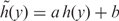to approximate a log2 transformation for probes with high signal intensities (Linear transformation will not affect the variance stabilization). This enables the direct incorporation of the VST results into existing procedures for normalization and analysis. Figure 1B shows an example of the relationship between a VST transform and a log2 transform. It indicates that the VST-transform is very close to log2 when the probe intensity measurement value is high (larger than 2⁹ in this case), but compressed for low-intensity values.

Evaluation data sets and computational platform

Currently, there are few publicly available benchmark data sets to evaluate the Illumina platform; as far as we know, none of them is provided with bead-level output under differentially expressed conditions. Thus, we used two data sets to evaluate the VST algorithm.

The Kruglyak data measured the Total Human Reference RNA (Stratagene, Inc.) on one microarray using Illumina Sentrix Human-6 Expression BeadChip version 1.0 (12). They were the only public data we could find that output the hybridization intensities of individual beads. Raw hybridization intensities provided by Illumina were used without any further preprocessing. We used this data set to evaluate the effectiveness of different variance stabilization methods on bead replicates.

The Barnes data set (4) measured a titration series (alternatively, it can be viewed as a dilution series) of two human tissues: blood and placenta. There are six samples with the titration ratios of blood and placenta at 100:0, 95:5, 75:25, 50:50, 25:75 and 0:100. The samples were hybridized on the pre-released HumanRef-8 BeadChip version 1.0 (Illumina, Inc.) in duplicate. We noticed that the number of bead-per-probe type of the Barnes data set ranges from 19 (25% quantile) to 30 (75% quantile), which is lower than the commercially released versions. We used this data set to evaluate the detection of differentially expressed genes. To give the hybridization intensities a meaningful origin for the titration analysis, the Barnes data have been background-adjusted by subtracting the median of negative control probes (using non-detected probes as a proxy).

As the Illumina BeadStudio output file has included the estimation of the mean (the AVG_Signal column, which is the mean after removing outliers as estimated by 3 MADs) and the standard error of the mean (the BEAD_STDERR column, which is the standard error of the mean after removing the outliers) of each probe, we did not recalculate the mean and standard deviation directly from the bead-level data. First, we translated the standard error of the mean into the standard deviation: 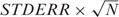, where STDERR is the standard error of the mean, and N is the number of the beads for the probe; then we fitted the probe mean and variance relations, as shown in Equation (4).

For normalization, we used quantile normalization (13); thus, the BeadStudio normalization option was turned off. A study of the combinatorial interplay between the background correction, data transformation, normalization and differential detection methods, similar to the work of Choe et al. (14), is beyond the scope of this paper.

We used the functions in the ‘lumi’ Bioconductor package to do all the processing (available at www.bioconductor.org). A vignette that includes all the scripts to process the Barnes data set is in the Supplementary Data. Users can easily reproduce the results shown in the following section, and check the results under different parameter settings.

RESULTS

VST stabilizes variances of bead-replicates within an array

To evaluate the variance-stabilizing capability of different data transformations, we first evaluated their effects on bead-level replicates within a single microarray by the following steps: (i) Specify the transforming function, h(y); for VST, it is estimated using the probe intensity mean and variance; (ii) transform the intensity value of each bead-replicate, y_i, into ; and (iii) Estimate the variance and mean of the transformed value . After an optimal VST, we would expect the intensity mean and variance of the transformed values for the different probes on a chip to be independent of each other, i.e. the variance does not change with the intensity of the measurement.

Figure 2 compares the variance-stabilization effects of the bead-level Kruglyak data (one microarray) for different methods: raw, VST, log2 and cubic root. Figure 2A shows that the variance increases significantly with the increase of intensity ranking of the raw data. Comparing the ranking of the intensity mean and standard deviation relations of the transformed data (Figure 2B–D), the VST method outperforms the other two commonly used transform methods: the Log2 transform does not perform well for the probes with low ranking (low-intensity signals), whereas the cubic root transform does not stabilize the variance for the probes with high ranking (high-intensity signals). Note that the VSN method is not applicable when only one microarray is available.

Figure 2.

Rank of mean and standard deviation relations of the bead-level data. Each data point represents a probe (usually over 30 beads are used to calculate the statistics of each probe). The red dots depict the running median estimator (window-width 10%). (A) Raw data without transform; (B) VST- transformed; (C) log2-transformed; (D) Cubic root-transformed. For an optimal VST, we would expect there to be no trend between the rank of the mean and the standard deviation.

The effect of VST on between-array technical replicates

We have shown the effectiveness of VST for stabilizing variances of technical replicates within one microarray. Next, we took a pair of technically replicated microarrays (titration ration of 100:0) in the Barnes data set to evaluate the data transformation effect on between-array replicates. Similar to the previous bead-level evaluation, we also investigated the mean and standard deviation relations of the technical replicate microarrays after preprocessing. Figure 3 compares the mean and standard deviation relations of technical replicates processed by different methods. Data processed with the VST-quantile (VST transformation followed by quantile-normalization) method and VSN-techReplicate (VSN applied separately to each technical-replicate pair) result in relatively evenly distributed variance over the ranking of the intensity mean. In contrast, the log2-quantile processed data shows high variance at low ranking (low-intensity values). Note that the Barnes data set, where a larger number of genes are differentially expressed (4), poses a significant challenge (Figure 3D) to the regular VSN procedure (VSN applied to all the arrays in the data set): VSN requires the assumption that most of the genes across different arrays are not differentially expressed.

Figure 3.

Rank of mean and standard deviation relations of the technical replicate microarrays after preprocessing. The red dots depict the running median estimator (window-width 10%). Plotted are two 100:0 (blood:placenta) replicates in the Barnes data set, which are separately located at two HumanRef-8 BeadChips. (A) VST- transformed and quantile-normalized; (B) log2-transformed and quantile-normalized; (C) Regular VSN-processed. (D) VSN-techReplicate method performed VSN only using the pair of technical replicates. Note: for Figure A–C, all six pairs of samples were preprocessed together, although only the replicates of the 100:0 group were plotted.

Furthermore, VST improves the consistency of technical replicates. Figure 4 shows the boxplot of correlation coefficients from six different pairs of technical replicates after preprocessing. We can see that the VST-quantile method results in the best correlation between technical replicates after preprocessing. Again, VSN-techReplicate procedure outperforms the regular VSN because of the VSN assumption discussed above. In contrast, VST uses technical replicates within each array to estimate optimal transformation parameters, and thus it is not complicated by the relationship across arrays.

Figure 4.

Comparison of the correlation between technical replicates of six different pairs of chips after preprocessing. The VSN-techReplicate indicates that the VSN method was separately applied to each pair of technical replicates. All other methods were applied to the whole data set of six pairs.

VST improves the signal-to-noise ratio

In the previous section, we evaluated the effects of variance-stabilizing techniques on improving the reproducibility of between-array technical replicates. However, this is only one of the performance criteria that we need to assess: if one only considers making the results of each experiment similar, then an algorithm making all results the same would be the best, which is not our intent. Therefore, we also compared the variation between groups versus the variation within groups:

This is equivalent to assessing the signal-to-noise ratio. For N groups, by generalization, we used the F-statistic as an approximation. Figure 5 shows the cumulative distribution of P-values obtained from F-tests using the Barnes data set; each titration ratio is treated as a group. Although the differences among the three methods are not very large, VST consistently outperforms the log2 and VSN methods. This indicates that VST does not destroy the variations between groups but it does improve the consistency within each group. As such, VST apparently improves differential detection (the capability of finding more significant genes using the same F-test and cutoff). Next, we investigated whether the differentially expressed genes detected following the VST transformation are false positives.

Figure 5.

The cumulative distribution of P-values obtained from F-tests. These are measures of the ratio of the between-group variation and within-group variation, or, in other words, the signal-to-noise ratio. Here, a ‘group’ means the samples with the same titration ratio.

VST reduces false positives of differentially expressed genes

To better evaluate the ‘real life’ performance of the VST algorithm, we need to examine how it may facilitate the identification of differentially expressed genes. Currently, there is no spike-in data set (15) available for the Illumina platform. We have selected the Barnes data set, which is a series titration of two tissues at five different titrations, for this purpose. For the Barnes data set, because we do not know which of the signals are coming from ‘true’ differentially expressed genes, we cannot use an ROC curve (15) to compare the performance of different algorithms. Instead, we assume that if a probe demonstrates the concordant titration behavior across all six conditions, then it is more likely to be a true answer. Following Barnes et al. (4), we defined a concordant probe as a signal from a probe with a correlation coefficient larger than 0.8 between the normalized intensity profile and the real titration profile (six titration ratios with two replicates at each titration).

The probes selected by the F-test in Figure 5 only satisfy the condition that at least one of the six groups is different from the others; it does not require concordance with the titration profile. Next, we want to further evaluate how many of the most significant probes (ranked by F-test and called ‘top probes’ in Figures 6 and 7) are concordant probes, as shown in Figure 6. If a selected differentially expressed probe is also a concordant one, it is more likely to be truly differentially expressed; we use this criterion as a proxy for false positives by the F-test. We can see that VST-transformed data consistently have an ∼5% increase of the concordant probes among the top significant probes based on the F-test.

Figure 6.

The percentage of concordant probes among the top probes by ranking the F-test P-values. The concordant probes are defined as those with correlation coefficients between the gene expression profile (measured by probe intensities) and the titration profile larger than 0.8. Note that the F-test P-value of the 3000th probe is 0.00019, 0.00022 and 0.00023 (VST-quantile, log2-quantile and VSN, respectively).

Figure 7.

The percentage of concordant probes among the top probes by ranking the t-test p-values estimated by ‘limma’ (16). The concordant probes are defined as those with correlation coefficients between the gene expression profile (measured by probe intensities) and the titration profile larger than 0.8. Note that the P-value of the 1000th probe is 0.0013, 0.0079 and 0.0040 (VST-quantile, log2-quantile, and VSN respectively).

The most commonly encountered task of microarray data analysis is to compare a treatment condition to a control condition, which is usually done by using a statistical model to adjust the t-test score (16). To mimic real-life applications, we selected for comparison the samples with the smallest titration difference in the Barnes data set (the most challenging comparison), i.e. the samples with the titration ratios of 100:0 and 95:5 (each condition has two technical replicates). Users can easily select other pairs and rerun the vignette (see Supplementary Data) to investigate the corresponding results. We used the Bioconductor ‘limma’ package (16) to estimate the P-values of the two-condition comparison. Figure 7 shows the percentage of concordant probes among the top probes by ranking the probes’ P-values from lowest to highest. Again, the VST-Quantile method clearly outperforms the log2-quantile and VSN methods. This suggests that by appropriate data transformation, the statistical test is more likely to pick up the true answers (the ones showing the titration behavior). As such, VST helps to reduce false-positive identifications.

DISCUSSION AND CONCLUSION

Based on the two data sets and different evaluation criteria, we list evidences that the VST transformation successfully stabilizes the variance both within each microarray and between technical replicates over a wide range of intensities. In essence, VST uses an error model that provides a bias against low-intensity values, as these signals are prone to measurement noise. As a result, the VST transformation improves the detection of differentially expressed genes and reduces the selection of discordance genes (more likely to be false positives) in the Barnes data set. VST can be viewed as a generalized log2 transformation, fine-tuned for the noise characteristics of each array based on the model specified in Equation (1).

Table 1 compares VST with VSN. Both are based on the general error model in Equation (1); the major difference is that VST estimates the parameters in Equation (4) by using intra-array technical replicates as a proxy, while VSN estimates the parameters using inter-array measurements by assuming that a majority of the genes are not differentially expressed and thus can be treated as technical replicates. The assumption by VSN, whenever challenged as in the Barnes data set, can lead to suboptimal model fitting. Another difference is that VSN must rely upon an integrated normalization method, since it uses inter-array measurements. In contrast, VST has the flexibility to work with any other normalization method in tandem. In addition, the linear fitting method used in VST is simpler, faster and can be more robust than the numeric optimization of the non-quadratic log-likelihood in VSN. A very significant part of the improved performance of VST plus normalization compared with VSN is that the number of beads used for estimating the variance function of Illumina arrays is far larger than the number of microarrays typically available for use with the VSN method. This fact alone accounts for much of the more robust behavior of the VST method for the transformation of data from the Illumina platform. However, VST is not directly applicable to spotted arrays or Affymetrix arrays, where the intra-array technical replicates are not abundant.

Table 1.

Comparisons of log2, VSN andVST

	log2	VSN	VST
Error model for each individual array	None	Equation (1)	Equation (1)
Allows negative values as inputs	No	Yes	Yes
Parameters in the model estimated from	None	Between-array replicates	Within-array replicates
Parameter estimation method	Fixed mathematical transformation	Maximum likelihood integrated with normalization	Linear fitting
Requires built-in normalization	No	Yes	No
Assumptions of the replicates	None	Most of the probes are not differentially expressed across arrays; thus, they can be treated as replicates.	No such assumption is required because technical replicates of the probes in the same array are used.
Observed or assumed replicates	Not used	Usually <12	Usually over 30

In practice, people often turn off the background subtraction (or even add a positive offset to the microarray measurement values) before they do a logarithm transformation in order to suppress the high variance at the low expression range. In such an empirical approach, the selection of the offset is arbitrary and might not provide uniform performance across chips and experiments. Thus, the final analysis results are very sensitive to which background correction method is used (17). Instead, VST generates an estimate of the offset c₂ [Equation (7)] based on the mean and variance relations v(u). The impact of different background correction methods on VST requires further investigation.

The VST method and a standard logarithm transformation are also closely related. After examining Equations (4) and (8), we find that the logarithm transformation is a special case of VST when c₃ = 0 or the measurement intensity is high. This explains the result in Figure 1B: for large u (intensity) values, the VST method converges to the results from the log transformation.

We have noticed that the bias introduced by VST tends to slightly over-suppress the measurements at the low end for some data sets; i.e. under-reporting the difference when the signal is close to the background. This phenomenon is due either to the current implementation or to the fact that real data is more complex than the assumed model in Equation (1). Further investigation is required. In practice, some caution might be necessary when one wants to focus attention on finding differential expression among these marginally expressed genes, although most researchers tend not to give priority to the genes expressed at a very low level compared with background noise.

As one reviewer pointed out, the Barnes data set can also be evaluated by looking at the correlation between the expression profile and the titration profile: a favorable data transformation method with low bias would improve the correlation. We investigated this and found that the VST-quantile-processed data have more probes with high correlation between the expression and titration profile. (See the Supplemental Data, Figure 3).

A data transformation procedure cannot be evaluated alone without using a normalization procedure. In the current evaluation, we used VST transformation followed by a quantile normalization procedure. The reason for this combination is to provide a more direct comparison with the popular log2-Quantile procedure. Other normalization methods can also be used together with VST transformation.

To deal with the heteroskedasticity problem, an alternative to data transformation is to abandon the canonical linear models that require making distribution assumptions. For example, the cyberT-test method (18) uses a moving window to reduce the dependency of variance on expression level. However, these ad hoc modifications cannot be easily generalized to complex experimental designs such as a mixed linear model, nor can they be used to calculate the statistical power of a given sample size.

SUPPLEMENTARY DATA

Supplementary Data are available at NAR Online.

REFERENCES

- 1.Kuhn K, Baker SC, Chudin E, Lieu MH, Oeser S, Bennett H, Rigault P, Barker D, McDaniel TK, et al. A novel, high-performance random array platform for quantitative gene expression profiling. Genome Res. 2004;14:2347–2356. doi: 10.1101/gr.2739104. [DOI] [PMC free article] [PubMed] [Google Scholar]
- 2.Brazma A, Hingamp P, Quackenbush J, Sherlock G, Spellman P, Stoeckert C, Aach J, Ansorge W, Ball CA, et al. Minimum information about a microarray experiment (MIAME)-toward standards for microarray data. Nat Genet. 2001;29:365–371. doi: 10.1038/ng1201-365. [DOI] [PubMed] [Google Scholar]
- 3.Du P, Kibbe WA, Lin SM. nuID: a universal naming scheme of oligonucleotides for Illumina, Affymetrix, and other microarrays. Biol. Direct. 2007;2:16. doi: 10.1186/1745-6150-2-16. [DOI] [PMC free article] [PubMed] [Google Scholar]
- 4.Barnes M, Freudenberg J, Thompson S, Aronow B, Pavlidis P. Experimental comparison and cross-validation of the Affymetrix and Illumina gene expression analysis platforms. Nucleic Acids Res. 2005;33:5914–5923. doi: 10.1093/nar/gki890. [DOI] [PMC free article] [PubMed] [Google Scholar]
- 5.Huang S, Yeo AA, Gelbert L, Lin X, Nisenbaum L, Bemis KG. At what scale should microarray data be analyzed? Am. J. Pharmacogenomics. 2004;4:129–139. doi: 10.2165/00129785-200404020-00007. [DOI] [PubMed] [Google Scholar]
- 6.Durbin BP, Hardin JS, Hawkins DM, Rocke DM. A variance-stabilizing transformation for gene-expression microarray data. Bioinformatics. 2002;18(Suppl. 1):S105–S110. doi: 10.1093/bioinformatics/18.suppl_1.s105. [DOI] [PubMed] [Google Scholar]
- 7.Huber W, von Heydebreck A, Sultmann H, Poustka A, Vingron M. Variance stabilization applied to microarray data calibration and to the quantification of differential expression. Bioinformatics. 2002;18(Suppl. 1):S96–S104. doi: 10.1093/bioinformatics/18.suppl_1.s96. [DOI] [PubMed] [Google Scholar]
- 8.Rocke DM, Durbin B. A model for measurement error for gene expression arrays. J. Comput. Biol. 2001;8:557–569. doi: 10.1089/106652701753307485. [DOI] [PubMed] [Google Scholar]
- 9.Tibshirani R. Estimating transformations for regression via additivity and variance stabilization. J. Am. Stat. Assoc. 1988;83:394–405. [Google Scholar]
- 10.Durbin B, Rocke DM. Estimation of transformation parameters for microarray data. Bioinformatics. 2003;19:1360–1367. doi: 10.1093/bioinformatics/btg178. [DOI] [PubMed] [Google Scholar]
- 11.Rocke DM, Durbin B. Approximate variance-stabilizing transformations for gene-expression microarray data. Bioinformatics. 2003;19:966–972. doi: 10.1093/bioinformatics/btg107. [DOI] [PubMed] [Google Scholar]
- 12.Chudin E, Kruglyak S, Baker SC, Oeser S, Barker D, McDaniel TK. A model of technical variation of microarray signals. J. Comput. Biol. 2006;13:996–1003. doi: 10.1089/cmb.2006.13.996. [DOI] [PubMed] [Google Scholar]
- 13.Bolstad BM, Irizarry RA, Astrand M, Speed TP. A comparison of normalization methods for high density oligonucleotide array data based on variance and bias. Bioinformatics. 2003;19:185–193. doi: 10.1093/bioinformatics/19.2.185. [DOI] [PubMed] [Google Scholar]
- 14.Choe SE, Boutros M, Michelson AM, Church GM, Halfon MS. Preferred analysis methods for Affymetrix GeneChips revealed by a wholly defined control dataset. Genome Biol. 2005;6:R16. doi: 10.1186/gb-2005-6-2-r16. [DOI] [PMC free article] [PubMed] [Google Scholar]
- 15.Irizarry RA, Bolstad BM, Collin F, Cope LM, Hobbs B, Speed TP. Summaries of Affymetrix GeneChip probe level data. Nucleic Acids Res. 2003;31:e15. doi: 10.1093/nar/gng015. [DOI] [PMC free article] [PubMed] [Google Scholar]
- 16.Smyth GK. Linear models and empirical Bayes methods for assessing differential expression in microarray experiments. Stat. Appl. Genet. Mol. Biol. 2004;3 doi: 10.2202/1544-6115.1027. Article3. [DOI] [PubMed] [Google Scholar]
- 17.Ritchie ME, Silver J, Oshlack A, Holmes M, Diyagama D, Holloway A, Smyth GK. A comparison of background correction methods for two-colour microarrays. Bioinformatics. 2007;23:2700–2707. doi: 10.1093/bioinformatics/btm412. [DOI] [PubMed] [Google Scholar]
- 18.Baldi P, Long AD. A Bayesian framework for the analysis of microarray expression data: regularized t -test and statistical inferences of gene changes. Bioinformatics. 2001;17:509–519. doi: 10.1093/bioinformatics/17.6.509. [DOI] [PubMed] [Google Scholar]
Associated Data
This section collects any data citations, data availability statements, or supplementary materials included in this article.