

Abstract
The rise in the number of functionally uncharacterized protein structures is increasing the demand for structure-based methods for functional annotation. Here, we describe a method for predicting the location of a binding site of a given type on a target protein structure. The method begins by constructing a scoring function, followed by a Monte Carlo optimization, to find a good scoring patch on the protein surface. The scoring function is a weighted linear combination of the z-scores of various properties of protein structure and sequence, including amino acid residue conservation, compactness, protrusion, convexity, rigidity, hydrophobicity, and charge density; the weights are calculated from a set of previously identified instances of the binding-site type on known protein structures. The scoring function can easily incorporate different types of information useful in localization, thus increasing the applicability and accuracy of the approach. To test the method, 1008 known protein structures were split into 20 different groups according to the type of the bound ligand. For nonsugar ligands, such as various nucleotides, binding sites were correctly identified in 55%–73% of the cases. The method is completely automated (http://salilab.org/patcher) and can be applied on a large scale in a structural genomics setting.
Keywords: protein function annotation, small ligand binding-site localization
Many protein targets of structural biologists are no longer chosen because of their function, but rather by their location in the protein sequence-structure space (Burley et al. 1999; Brenner 2000, 2001; Sali 2001; Vitkup et al. 2001; Chance et al. 2002; Goldsmith-Fischman and Honig 2003). Therefore, the number of functionally uncharacterized protein structures is growing. Of the 36,606 entries in the Protein Data Bank (PDB) (Kouranov et al. 2006) as of February 23, 2006, 1407 structures were deposited by structural genomics consortia, 985 (70%) of which had an unknown function according to the HEADER record of their PDB files. In contrast, only 174 (0.5%) of the 35,199 protein structures solved outside of structural genomics had no functional annotations in their PDB files.
To classify the functions of thousands of uncharacterized protein structures that will become available over the next few years and millions of comparative models based on the known structures, automated structure-based functional annotation is required (Wallace et al. 1996, 1997; Kleywegt 1999; Thornton et al. 2000; Babbitt 2003; Laskowski et al. 2003). In particular, we need to be able to identify the locations and types of binding sites on a given structure, because the binding sites define the molecular function of a protein.
The most principled computational approach to predicting the molecular function is to dock a large library of potential ligands against the surface of the protein. In practice, because of the inaccuracies of the available scoring functions and difficulties in the conformational and configurational sampling, few such attempts have been made (Greenbaum et al. 2002; Macchiarulo et al. 2004). Furthermore, most docking programs require a specification of the location of the binding site as part of their input. Thus, the first step in ligand docking is usually to localize the likely binding site on the surface of the target protein. The binding sites are generally cavities on protein surfaces, often the largest ones (Kuntz et al. 1982; Laskowski et al. 1996; Liang et al. 1998; Brady and Stouten 2000). However, not all cavities on the surface of a protein are binding sites, and it is not well understood what distinguishes binding sites from other cavities (Ringe 1995). Mapping the surface of the protein with molecular probes, such as organic solvent molecules, and calculating energetically favorable locations for ligands helps to detect binding sites on the surface of a protein structure (Goodford 1985; Miranker and Karplus 1991; Silberstein et al. 2003). Other methods identify hot spots, defined as destabilizing residues on the surface of a protein that may therefore be part of a binding site (Elcock 2001).
One of the simplest bioinformatics approaches to localizing binding sites depends on the availability of a set of related sequences. The binding site is predicted to correspond to a set of contiguous surface residues that are also evolutionarily conserved in the corresponding multiple sequence alignment (Zvelebil et al. 1987; Mirny and Shakhnovich 1999; del Sol Mesa et al. 2003). This strategy works to some degree because evolution tends to conserve functionally important residues. Another approach uses a principal components analysis to find a set of spatially local positions in a multiple sequence alignment whose clustering mimics the known functional classification of the group (Casari et al. 1995). A related approach, the evolutionary trace method, also exploits the conservation of function within a family and variation of function between families of a superfamily (Lichtarge et al. 1996; Aloy et al. 2001; Armon et al. 2001; Landgraf et al. 2001; Madabushi et al. 2002; del Sol Mesa et al. 2003; Yao et al. 2003), benefiting from a multiple sequence alignment, the corresponding phylogenetic tree, and the three-dimensional structure of at least one member of the superfamily. The conservation-based and evolutionary trace methods appear to have similar accuracies (del Sol Mesa et al. 2003), although a rigorous assessment is difficult because of its dependence on the testing data set and the testing criteria.
The conservation-based and evolutionary trace methods listed above can be applied even when binding-site locations are unknown for all homologs in the set. In contrast, homology-based approaches use information about related protein sequences and structures with known binding-site locations. Detection of sequence similarity between an uncharacterized target and a characterized template has been the most frequently used method to identify the locations of functional sites (Bork et al. 1998). However, these methods become less accurate as the evolutionary distance between the two proteins increases (Eisenstein et al. 2000; Moult and Melamud 2000; DeWeese-Scott and Moult 2004). In addition, while the functional binding sites can be detected by looking at the sequence conservation, many drugs interfere with the protein function by binding at the secondary binding sites (Hardy and Wells 2004).
At the sequence level, local sequence patterns have been successfully applied to function prediction even in the absence of high-sequence similarity (Bairoch and Bucher 1994). At the structure level, 3D-motifs (i.e., conserved spatial arrangements of side chains, residues, and/or secondary structure segments) have also been successfully used to identify binding sites of the same type in proteins with different folds (Artymiuk et al. 1994; Wallace et al. 1996, 1997; Kleywegt 1999; Oldfield 2002; Stark and Russell 2003; Stark et al. 2003). Another related approach to comparing binding sites relies on five different chemical descriptors that describe the cavity of a protein, thus allowing a comparison of binding sites independently from sequence and structure similarities (Schmitt et al. 2002). Several other approaches that use invariant physical properties of the binding site were also described for characterization of protein–ligand, protein–protein, and protein–DNA interactions (Rosen et al. 1998; Pawlowski and Godzik 2001; Chakrabarti and Janin 2002; Kinoshita and Nakamura 2003; Ahmad et al. 2004; Neuvirth et al. 2004; Deremble and Lavery 2005).
While the existing methods provide useful ways to identify and describe binding sites, the problem of accurate identification of the location of a binding site of a given type on a target protein structure is not solved. We suggest that a method capable of integrating a variety of different types of information about the given protein structure, its binding site, and its homologs is likely to do better than any one of the methods based on a subset of information. We describe here such a method. The integration is expressed as an optimization problem that depends on a representation of protein-binding sites, a composite scoring function for evaluating the likelihood that any patch of residues is a binding site of the required type, and a sampling protocol that searches for good scoring patches (▶; see Materials and methods).
Figure 1.

(A) Scheme of the integration of different properties into a single scoring function to localize the binding site of a given type in a target protein structure (see Materials and methods). (B) Flowchart of the optimization protocol (see Materials and methods).
Below, we describe the localization method and the benchmarking criteria (Materials and methods). Then, we assess the accuracy of the method and illustrate it by several sample applications (Results). We conclude by discussing the implications of the approach for automated functional annotation of proteins (Discussion).
Materials and methods
We aim to maximize the accuracy of the localization of a binding site of known type on a target protein structure by combining varied information about the binding site (▶). This aim is achieved by expressing the problem as an optimization problem, which requires a representation of the protein and its binding site, a scoring function, and an optimization algorithm. We describe the three aspects of the approach next.
Binding-site representation and patch definition
The binding site is predicted by identifying the patch with the optimal score. A patch consists of a set of contiguous surface residues. By definition, a surface residue must have at least one atom with accessible solvent area (ASA) larger than 2 Å2. A residue that is not on the surface is a core residue. Two surface residues are contiguous if the closest exposed atoms from the two residues are <6 Å apart.
Composite scoring function
The scoring function is a weighted combination of seven properties. These properties were chosen to represent a variety of features of binding sites that generally distinguish them from the rest of the protein, such as their evolution (sequence conservation), shape (compactness, protrusion, and convexity), energetics (hydrophobicity and charge density), and dynamics (rigidity).
Sequence conservation
The first property is based on the observation that most binding sites are likely to be relatively conserved in sequence because of the evolutionary pressure to keep the binding sites intact (Introduction). Sequence conservation of a given patch is defined as the average Shannon entropy (Shannon 1948) of the residues in the patch. The Shannon entropy at a given multiple sequence alignment position is
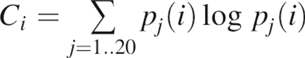 |
where pj(i) is the frequency of residue j at position i based on a multiple sequence alignment generated by the program PSI-BLAST, with default parameters except for the e-value threshold of 10−5. The search database is Uniprot with ∼3.2 million sequences (Wu et al. 2006); the query sequence is the target protein whose binding site is being localized.
Compactness
To encode the shape of the patch, compactness is defined as the average distance between the residues that form a patch:
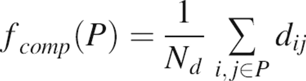 |
where Nd is a normalization factor corresponding to the number of considered distances (i.e.,  ) and dij is the distance between the two closest surface atoms of residues i and j in the patch P.
Protrusion
Patch protrusion is defined as the percentage of protruding residues in the patch (▶). A residue is protruding if at least 50% of its atoms are protruding. An atom is protruding if the number of neighboring atoms (i.e., the number of atoms that lie between 8 and 12 Å from the query atom) is <120. These two parameters were determined by visual inspection of protein structures.
Figure 2.
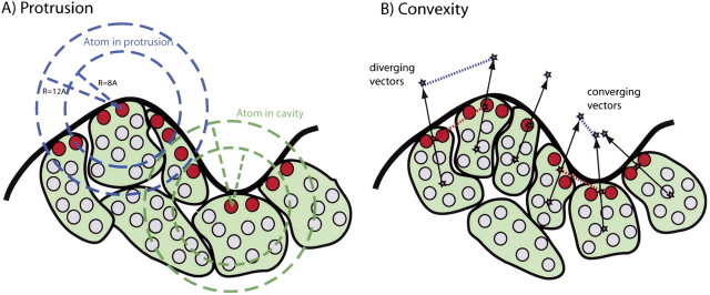
Schematic representations of protrusion and convexity (see Materials and methods). (A) Protrusion is calculated by counting the number of neighboring atoms. The atom count is very different for a protruding atom and an atom in a cavity. (B) Convexity is determined by using three different types of reference points. For every exposed residue, the exposed and buried centroids (represented by the red and the gray stars) are the geometrical centers of the exposed and buried atoms, respectively. The “solvent point” (blue star) is located on the exposed side of a line connecting the buried and exposed centroids 3 Å away from the exposed centroid.
Convexity
Another geometrical property, patch convexity, is determined by averaging the residue convexity for each residue in the patch (▶). The convexity of residue i is obtained by considering Ni nearest-neighbor residue pairs involving residue i (n.n.res.):
 |
where d solv ij and d exp ij are the distances between the “solvent points” and “exposed centroids” of residues i and j, respectively (▶).
Rigidity
Flexibility of the native structure is likely to have a role in many protein–ligand interactions. The rigidity of a patch is calculated as the average B-factor of the exposed atoms involved in the patch. All B-factors are obtained from the crystallographic PDB files. A measure of flexibility determined by NMR spectroscopy could also be used.
Hydrophobicity
The hydrophobic effect frequently plays an important role in protein–ligand recognition. The hydrophobicity of a patch is calculated as the average hydrophobicity of the residues in the patch. The residue hydrophobicity is obtained from the experimentally derived scale of Fauchere (Fauchere and Pliska 1983).
Charge density
Atomic charges are many times responsible for the specificity of protein–ligand recognition. Charge density of a patch is the sum of charges for its exposed atoms divided by the solvent accessibility area of the patch. Atomic charges are obtained from the CHARMM22 force field (MacKerell et al. 1998).
Scoring function 1: Linear model
The linear scoring function favors binding-site predictions that maximize the difference observed between random patches and known examples of a given binding-site type. First, each one of the seven properties defined above is normalized by transforming its value f into a z-score 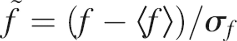 . Both the average <f> and the standard deviation σf are obtained from a sample of 1000 random patches, generated as described below. The normalization of the seven properties is useful because it puts them all on the common scale for subsequent comparisons.
Second, the seven z-scores are summed
 |
where k denotes the property type and P is a patch. The weights wk determine the relative importance of each property in the search for the binding-site location. Both the absolute values |W k| and the signs of the weights sign wk are crucial; the relative magnitude controls the importance that each single property has in the scoring function, while the sign controls whether the property is maximized or minimized.
This scoring function can be used for different types of binding sites by adjusting the property weights. Here, we calculate the weights independently for each type of the binding site from a sample of structurally defined binding sites of the required type. The weight of each property is calculated as the average of the z-scores obtained from a training set of known binding sites {P i} of the given type:
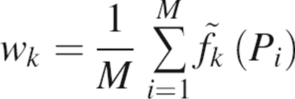 |
where M is the number of binding sites in the training set. Therefore, properties that have consistently positive (negative) z-scores will be positively (negatively) weighted and properties with z-scores fluctuating around zero will have small weights. Each binding-site type is described quantitatively by the seven property weights wk, forming a fingerprint of the binding site. Unless otherwise noted, we use scoring function 1 in this work.
Scoring function 2: Quadratic model
The quadratic scoring function favors binding-site predictions that are similar to known examples of a given binding-site type:
 |
where λk and σk are the average and standard deviation of property k for the known binding sites (positives), respectively. The weight of property k depends on the dissimilarity between the distributions of the property for the known binding sites and random patches as quantified by the Fisher's discriminant ratio (Theodoridis and Koutroumbas 1999):
 |
where λ′k and σ′k are the average and standard deviation for the random patches (negatives), respectively.
Patch optimization
To find the optimal patch corresponding to the maximum of the scoring function, we need to explore the space of all possible patches. Unfortunately, given the limitations of computer power, this problem generally cannot be solved by an exhaustive enumeration of all patches. Thus, we used stochastic Monte Carlo Simulated Annealing (MCSA) optimization (▶; Kirkpatrick et al. 1983).
The first step in the MCSA optimization algorithm is the generation of an initial random patch. First, a surface residue is randomly selected to be the seed residue of a patch. Next, other contiguous residues are sequentially added to the patch until the patch consists of a predefined number of residues. The number of residues in a given patch is a random number from a uniform distribution defined by a set of known binding sites of the required type; in particular, the average and range of the uniform distribution were set to the average and twice the standard deviation of the binding-site size for the sample.
Next, the initial random patch is modified iteratively, by repetitive application of a move that involves a random addition and deletion of a residue from the patch. Only moves that do not destroy the contiguity of the patch are considered. The difference in the scores after and before the move, ΔF(P), is recorded. The move is accepted according to the standard Metropolis criterion with the following probability (Metropolis et al. 1953):
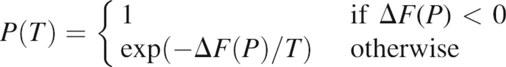 |
The Monte Carlo temperature T plays a major role in the MCSA. At high values of T, most moves are accepted, without strongly discriminating between uphill and downhill moves. At low T, primarily moves that decrease the score are accepted. The initial temperature was set to 1 and decreased at each minimization step by a factor of 0.999. Each optimization consisted of 10,000 such iterations. For each binding-site localization, 100 optimizations are performed, starting each time with a different, randomly selected seed residue.
Testing binding-site localization
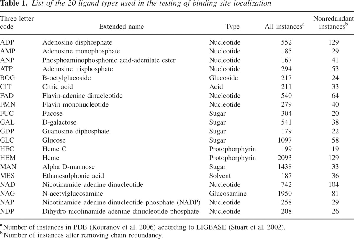
Testing sets of binding sites
We relied on the LIGBASE database (November 2003) (Stuart et al. 2002) to extract a list of binding sites from protein structures deposited in the PDB. A binding site is defined as all of the protein residues with at least one atom within 5Å of any of the ligand atoms. We restrict the data set to 20 different ligands of 10 or more heavy atoms that occur >100 times in LIGBASE. The set contains biologically relevant molecules (such as ATP, NAD, and sugars), but excludes ions and very small molecules. To avoid redundancy, we filtered the sample proteins so that all pairs of accepted structures satisfied the following three conditions: (1) The fraction of the Cα atoms that superpose within 4 Å is <90%, (2) the corresponding Cα RMSD is larger than 2 Å, and (3) sequence identity is <30%; alignments in DBAli (Marti-Renom et al. 2001) were used for this filtering. Finally, when more than one ligand interacted with a single chain, only one binding site was selected randomly (▶).
Table 1.
List of the 20 ligand types used in the testing of binding site localization
Testing protocol
To test the method, we used the jackknife protocol in which the structure whose binding site was localized was not used in the calculation of the scoring function parameters.
Accuracy of predictions
The accuracy of the localization prediction is assessed by an overlap between the actual and predicted binding sites. Given two patches, P1 and P2, with a number of residues, N1 and N2, respectively, the overlap between them is
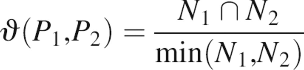 |
where N1 ∩ N2 is the number of overlapping residues and min(N1,N2) is their minimum value. The overlap of two patches is 1 if they are identical or one patch is completely contained within the other. The overlap is 0 if there are no residues in the intersection between the two.
For each test set, the overall accuracy of predictions is defined as the fraction of binding sites correctly localized. A binding site is considered correctly localized if the overlap ϑ of the best scoring patch with the actual binding site is greater than a predefined cutoff ϑ 0. Unless otherwise specified, we use ϑ 0 = 0.5.
Accuracy of random patches as a control
The difficulty of localization correlates with a variety of attributes, such as the average sizes of the protein, binding site, and the optimized patch. Some ligands may bind prevalently to large multidomain proteins, where the localization of the binding site is statistically more difficult because there are more nonbinding than binding residues compared with smaller proteins. For this reason, we compare the accuracy of localization relative to the accuracy obtained by randomly selecting a surface patch. The random patches correspond to the starting patches for the MCSA optimization.
Results
We now validate our optimization algorithm with an ideal scoring function and then we optimize the scoring function weights for all of the binding-site types considered in this paper (▶). Finally, after describing a sample binding-site localization, we assess the performance of our method with the aid of the whole testing data set.
Testing the optimization algorithm
It is necessary, although not sufficient, that a good optimizer finds a substantially correct solution when an ideal scoring function is used. We tested our MCSA sampling protocol with a scoring function that corresponds to the native overlap between a scored patch and the actual binding site. Otherwise, the default values of various parameters, such as the initial temperature and the temperature-scaling factor, were used (see Materials and methods). For a small number of arbitrarily chosen test cases, the known global minimum is almost always reached in 3000–4000 MC steps (▶). Moreover, even for realistic scoring functions, the algorithm tends to produce the same best-scoring solution for different, randomly selected starting patches. Therefore, we conclude that the optimizer is not likely to limit the accuracy of our predictions.
Figure 3.

Patch overlap as a function of the iteration number during a simulated annealing optimization. To test the efficiency of the MCSA protocol, the scoring function was replaced with the patch overlap. Under these ideal conditions, the program always retrieves the correct solution. The test involves predicting the location of the NAD binding site on dihydropteridine reductase (PDB ID 1dhr).
Property distributions and fingerprints
As described in Materials and methods, the scoring function is either a linear combination of individual property scores (linear model) or a linear combination of terms quadratic in the property scores (quadratic model). The weights and the other parameters are calculated from the distribution of the properties of the known binding sites and random patches. While random patches do not depend on the type of ligand, the distribution for known binding sites is specific to the binding-site type.
As an example, we describe the distribution of the NAD binding-site properties (▶). The z-scores of sequence conservation, hydrophobicity, protrusion, and convexity are consistently negative or positive for most of the protein–NAD complexes in our training data set. Accordingly, these properties will be important in discriminating a binding site from a random patch and should contribute to the scoring function more than the properties that are similar between the actual binding sites and random patches. The less discriminating properties include the compactness, charge density, and rigidity. The average of their z-scores is close to 0, varying from positive to negative values for the different known protein–NAD complexes.
Figure 4.

Distributions of the NAD binding-site properties. All the properties have a unimodal distribution. Properties having their peak around zero (i.e., compactness, protrusion, rigidity, and charge density) are less informative than those with their peak far from zero (i.e., conservation, hydrophobicity, and convexity).
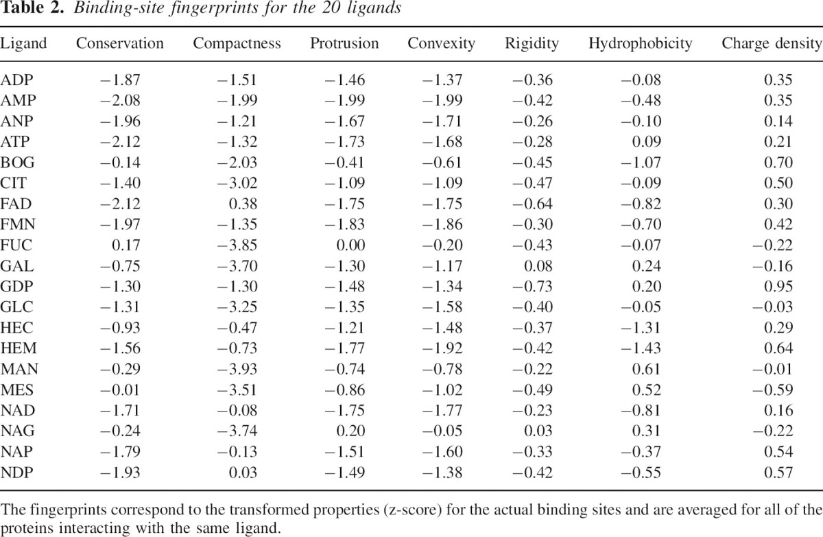
We determined the property weights for all 20 binding-site types considered in this paper (▶; see Materials and methods). For some properties, the seven z-scores are consistently positive or negative, while others change sign for different ligands. For example, rigidity of all binding-site types is consistently higher than that of a random surface patch, while the sequence is usually more conserved, although it can also be slightly more variable for ligands such as fucose and mannose. This difference in the distributions is reflected in the weights and, in the case of the quadratic model, in the other parameters of the scoring function. The set of parameters determined from a given training set of binding sites is specific to the corresponding ligand type and constitutes the fingerprint of the ligand (▶).
Table 2.
Binding-site fingerprints for the 20 ligands
Fingerprints and ligand similarity
In general, similar ligands should bind to similar binding sites and should therefore have similar fingerprints. We explored whether this is actually the case by clustering the fingerprints. We calculated a dendrogram of fingerprints, based on the Euclidean distances between pairs of fingerprints (▶). Similar ligands indeed tend to cluster together. For example, ligands containing the adenine moiety, such as ADP, ANP, and ATP, cluster in the lower arm of the tree, while sugars such as fucose, mannose, and glucose cluster in the upper arm. This clustering of the ligands by their fingerprints demonstrates that the fingerprints capture characteristics of the ligands, even though these characteristics were not used in the fingerprint construction.
Figure 5.

Clustering of ligands according to their binding site fingerprints (▶). The distance between two ligands has been calculated as the Euclidean distance between their fingerprints and the tree was obtained with Phylip (J. Felsenstein, University of Washington, Seattle). Ligands that cluster together have similar binding sites. While ligands with the adenine moiety are close to each other, sugars are spread more broadly (Results).
An example: Dihydropteridine reductase
We illustrate our method for binding-site localization by its application to the dihydropteridine reductase enzyme (DHPR) that binds the NAD cofactor. NAD binding-site position was determined by comparison with the corresponding native structure of the protein–ligand complex extracted from the PDB (code 1dhr) (▶; Varughese et al. 1992). The ability of our method to localize the NAD binding site was assessed by comparing the overlap between the binding site and 100 independently optimized patches with the overlap between the binding site and 100 random surface patches (see Materials and methods).
Figure 6.

Detailed analysis of predictions for protein 1dhr. (A,B) In the top panels, the cofactor NAD is indicated in yellow, and the binding residues are in red. The actual location of the binding site (A) is very similar to the prediction (B). (C) Distribution of 100 optimized patches as a function of their overlap with the actual binding site. The distribution of the optimized patches (red curve) peaks at ∼1 (maximum overlap), while random patches (green curve) peak at ∼0 (no overlap). The optimizer is able to find the binding site, in most cases with an overlap larger than 0.5. (D) Scatter plot of the overlap vs. the score for the 100 optimized and random patches; the optimized patches have a lower score than random patches by construction (because of the optimization); moreover, they also have a higher overlap with the actual binding site.
The best-scoring binding-site prediction overlaps with the actual binding site for 10 of 11 residues (▶). Of the 100 independently predicted binding sites, ∼50% have an overlap larger than 0.8 and only ∼20% have an overlap below 0.5 (▶). In contrast, for random surface patches, 97% have an overlap of ≤0.4 and 47% of the patches have no overlap at all. These results clearly indicate that the predicted binding sites are much closer to the actual binding site than the randomly generated surface patches. Moreover, the correlation between the binding-site overlap and the score is higher for the binding-site predictions (0.74) than for the random surface patches (0.47) (▶). In summary, for this particular example, the scoring function is sufficiently accurate and the optimizer sufficiently thorough for correct binding-site localization.
Accuracy of localization estimated with the testing set
Best prediction
To objectively assess the accuracy of the method, we localized the binding sites for all proteins in the 20 data sets defined in Materials and methods (▶). Accuracy varies significantly, depending on the type of binding site localized (▶). For ligands such as ATP, NAD, and FAD, there is a clear difference between the accuracies of the predicted and random patches, indicating that the scoring function captures the salient features of these binding sites. For example, for the nicotinamide-adenine-dinucleotide (NAD), the accuracy of predicted patches (75%) is much higher than that of random patches (5%) (▶). In contrast, for ligands such as fucose, B-octylglucoside, and mannose, the accuracy of predicted patches is comparable to that of random patches.
Table 3.
Accuracy for the 20 ligand types calculated for a single prediction (top_1) as well as for the most accurate prediction of the 5 (top_5) and 10 (top_10) best-scoring patches
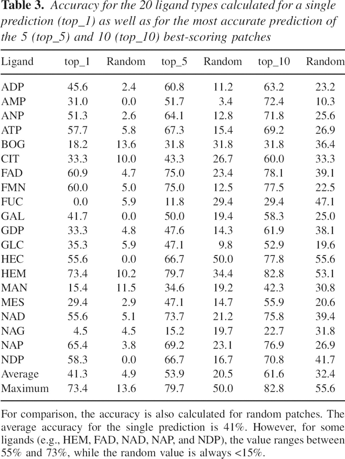
Figure 7.
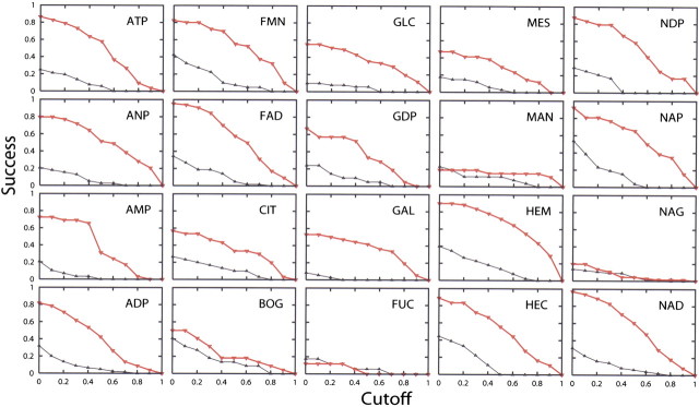
The accuracy of localization for the 20 ligand-binding sites as a function of the overlap cutoff ϑ 0, for both optimized patches (red curve) and random patches (black curve). As expected, for all ligands, the accuracy increases when ϑ 0 is decreased. The good localization of ligand binding sites for nucleotides, such as NAD, HEM, and NAP, contrasts with the poorer performance for sugars, such as GAL, MES, and FUC.
Suboptimal solutions
The binding site may not correspond to the best scoring patch, but merely to a good scoring patch. In such cases, the optimizer may still find the binding site, although the correct prediction will not be top-ranked. To quantify this possibility, we calculated the average accuracy of the most accurate of the five and 10 best scoring patches, both for the optimized and random patches. Compared with considering only the best-scoring patch, accuracy increases slightly for the optimized patches (from 70% for the single top prediction to 80% and 84% for the most accurate among the top five and 10 scoring patches, respectively) and much more for random patches (from 3% to 21% and 42%).
Accuracy as a function of the actual binding-site overlap cutoff
We investigated how the accuracy of localization is affected by the choice of the cutoff ϑ 0, which specifies the minimal degree of the predicted binding-site overlap with the actual binding site that is needed for a correct prediction (see Materials and methods). When the cutoff ϑ 0 is close to 1, only the best scoring patches that overlap completely with the known binding site will be counted as correct predictions. On the other hand, when ϑ 0 is close to 0, even patches that overlap only partially with the known binding site will be considered correct predictions. As expected, the accuracy of the method for every test set decreases as a function of the cutoff ϑ 0, both for the predicted binding sites and random patches (▶). For some ligands, almost all instances of their binding sites are correctly identified when the cutoff ϑ 0 is 0, which suggests that the best scoring patch is in the proximity of the known binding site rather than far away. In contrast, the poor performance for sugars is not affected by the choice of ϑ 0, indicating that the actual sugar binding-site locations are generally far from those of the best scoring predictions.
Discussion
We described, implemented, and benchmarked a method for integrating structure and sequence properties to predict the location of a binding site of specified type in a given protein structure. The method relies on a scoring function and a Monte Carlo optimization protocol to find a good scoring patch on the protein surface. The scoring function depends on z-scores of various properties of protein structure and sequence, including amino acid residue conservation, compactness, protrusion, convexity, rigidity, hydrophobicity, and charge density; the z-scores are calculated separately for each binding-site type from a set of previously characterized instances of the binding site on known protein structures (i.e., the training data set). We note that the binding site is not localized by the types of its residues, only by the degree of their conservation. Thus, we do not expect a strong dependence of localization on the degree of sequence similarity between the target sequence and the proteins in the training data set.
Combining information for localizing binding sites
Each of the previously described methods for localizing binding sites tends to rely on a relatively narrow set of considerations. For example, docking methods consider geometrical complementarity and physical interactions (Kuntz et al. 1982); some methods search for cavities (Laskowski et al. 1996), and others look specifically at the residue types in the binding site or at their particular features (geometric hashing) (Artymiuk et al. 1994; Wallace et al. 1996, 1997; Kleywegt 1999; Oldfield 2002; Stark and Russell 2003; Stark et al. 2003). These methods vary in terms of the ligand and protein properties used, the search algorithm, and even the primary goal (i.e., the identification of the ligand type or the localization of the binding site). An advantage of our approach is the ability to integrate information from different sources into a single scoring function. At least in principle, consideration of more information should lead to more accurate predictions.
Localizing a binding site by patch optimization
To make integration straightforward, we chose a single representation of the system for all of the properties (see Materials and methods). We represented the binding site as a patch of contiguous surface residues. Such patches have been used, for example, for the classification as well as prediction of protein–protein interactions by generating a limited number of patches and assessing them according to a user-defined scoring function (Jones and Thornton 1997a,b).
The number of possible patches on the surface is generally too large for an exhaustive enumeration. For noncontiguous patches, the number of different patches of r residues on a protein with n surface residues is  (e.g., ∼1022 for r = 15 and n = 200). The number of contiguous patches does not appear to be possible to estimate analytically, but it is still large enough to prevent an exhaustive enumeration. For this reason, we optimized a randomly created initial patch according to a scoring function rather than filter a manageable set of predefined patches by the scoring function. The advantages are that no manageable set of predefined patches needs to be constructed and that we are exploring the whole space of possible patches.
Performance of the optimizer
As in any optimization, our approach has two possible limitations: the optimizer and the scoring function. It is crucial to determine the power of the optimizer and the accuracy of the scoring function so that the future development effort is most productive. The role of the optimizer is to efficiently explore the space of all possible patches and find the best scoring one. For a given binding-site localization, when the optimization is carried out independently 100 times, starting with different random patches, the best-scoring solution is generally found in 30%–50% of the cases (e.g., ▶). Because the initial random patches are generated independently, it is very likely that the most populated solution, which usually corresponds to the best-scoring solution, is the global minimum. Thus, the optimizer is not likely to limit the accuracy of the method, and future efforts on improving the method should focus on improving the scoring function.
Modularity of the method
Our scoring functions rely on a set of properties that are linearly combined using weights specific to each binding-site type. This modularity of the scoring function allows for flexibly modifying, adding, and removing properties without affecting the encoding of the other properties and the optimization protocol. Consequently, different scoring functions, including different weights, can be easily compared. Another difference from some of the previous methods (Jones and Thornton 1997a,b) is that the weights are not chosen by the user based on their experience, but are calculated for each binding-site type by relying on a set of known structures containing the corresponding binding site. Given the chemical and physical diversity of possible ligands, the ability to encode their binding sites by the importance of different properties is expected to be an advantage over methods that do not differentiate between different ligands (e.g., looking for the largest surface cavity). This expectation is clearly borne out by the different calculated property weights for the different ligand binding-site types.
Linear scoring function
We implemented and compared two different scoring functions, linear and quadratic, in the binding-site properties. While the linear model is widely used in general discrimination problems because of its simplicity, more sophisticated scoring functions may be able to better identify the actual binding site as the best scoring patch. One potential problem of the linear model is that the binding-site properties are not restrained to specific target values. The predicted patches may have property values that are larger or smaller than those of the real binding sites. For example, if known sample binding sites correspond to a cavity, the predictions will tend to be the largest cavities on the surface because those are most different from the mostly flat random patches; this rationale may not always work correctly, especially for smaller ligands. A similar concern applies to the charge density of a patch.
Quadratic scoring function
We also tested a second scoring function where the properties are restrained relative to their distributions in the sample binding sites. We use restraints quadratic in the properties and centered on the averages of the corresponding sample distributions. While the linear model has seven parameters, there are 13 in the quadratic scoring function (seven parameters for the centers of the distributions and six for the weights). By construction, the best-scoring patches tend to have property values close to those in the sample binding sites. However, the accuracy of localization relying on the quadratic function is generally not as high as in the case of the linear model; for example, for ADP it drops from 46% for the linear model to 26% for the quadratic model. Perhaps this is explained by the fact that the quadratic function depends only on the known positive examples of the localized binding-site type, while the linear model depends on the difference between the training examples and random patches.
The accuracy depends on the predicted ligand binding-site type
The benchmark shows that the accuracy of our method varies for different binding-site types (▶). In particular, the accuracy of localizing sugar-binding sites is poor. It is known that sugars display a variety of binding modes and that the protein–sugar interactions are difficult to predict (Alberts et al. 2002). From a physical chemistry point of view, sugars interact with the protein through charged interactions that can be mediated by metal ions. From a biological point of view, sugars are used in a variety of biological processes. Such a variety of biological roles, which corresponds to a variety of binding modes, makes sugars a very difficult test set (del Sol Mesa et al. 2003). Incorporation of additional structural and sequence properties into the scoring function may result in improved localization.
Similar fingerprints produce similar localizations
We already showed that similar ligands have similar fingerprints (▶). We are now interested in whether similar fingerprints result in similar localization accuracies. If so, our localization method would be more useful for ligands with imprecisely determined fingerprints (i.e., ligands with few instances in the PDB). We localized five different ligands (i.e., ADP, FAD, FMN, HEM, and NAD) using their native fingerprints and the fingerprints for each one of the other four ligands. They all have similar fingerprints with high weights for conservation, protrusion, and convexity; HEM also depends strongly on hydrophobicity (▶). In general, using the native fingerprint results in the most accurate localization (data not shown). The non-native fingerprints reduce the accuracy of localization for 5%–15%. Considering that the localization accuracy ranges from 45% to 73%, fingerprints of similar ligands may therefore be used to localize binding sites for which only small training sets are available.
Toward the characterization of binding sites: Fingerprint specificity
Our current method has a precise and limited aim to localize the binding site for a given ligand type on a known protein structure. There are additional related problems, including predicting the type of the preferred ligand for a given binding site on a known structure. Properties that discriminate between binding sites and other regions of the protein, such as the seven properties used here, may also be effective in discriminating between different potential ligands for a given binding site. To find out how useful our fingerprints are for predicting the specificity of ligand binding, we performed the following experiment: For each of the 1008 structures in the 20 data sets, we assessed the scores of the 20 fingerprints applied to their native binding sites. Our fingerprints scored the native ligand best for 15.4% of the structures, which is three times better than the random rate (i.e., 1/20). Moreover, the success rate can only increase if we declare success when the native ligand is one of a few top-scoring ligands or when it is similar to the best-scoring ligand. Therefore, the fingerprints contain significant information about the specificity of the binding sites, although they are not sufficient on their own in their current form for a reliable identification of the ligand type.
We did not, however, address the most general question of predicting simultaneously both the location and type of the ligand binding sites on a given structure. A potential approach is to predict the best location for each available fingerprint, retain only the best scoring fingerprint for overlapping predicted locations, and finally apply a cutoff to the scores for the final prediction of both the location and type of the ligand-binding site. We do not expect that our current scoring function, developed for localization only, will be optimal for this integrated problem. For the current goal, the scoring function needs to maximize the difference between the tested binding site and a random patch. In contrast, for the prediction of the ligand type, the scoring function needs to maximize the difference between the alternative ligand types; thus, a different scoring function may be needed.
Some properties are more important than others
Because the localization problem was formulated as an optimization of a modular scoring function, it is relatively straightforward to further generalize the approach. For example, fingerprint weights for the conservation, protrusion, and concavity correlate with accuracy (Tables ▶, ▶). In contrast, fingerprint weights for compactness anti-correlate with accuracy (Tables ▶, ▶). Compactness is the only property that depends on the number of residues used to generate the patches and the only property designed specifically to restrain the shape of the patch rather than its location on the protein surface. Incorporating this feature via a linear term in the scoring function (i.e., the linear model) appears not to be the best solution.
We also analyzed how localization is affected by removing a property from the fingerprint. For ADP, for example, the properties with largest weights are conservation, protrusion, convexity, and compactness. The least-accurate localization is obtained when conservation is not used (30% vs. 46% for the full fingerprint), suggesting that conservation is the most important property in the ADP fingerprint. Localization accuracy also decreases without compactness (39%). Unexpectedly, localization accuracy slightly increases when protrusion and convexity are removed from the fingerprint (to 52% and 49%, respectively). This unexpected improvement might be a consequence of random error in the construction and assessment of fingerprints as well as of unaccounted correlations between the properties in the scoring function. Localization accuracy is essentially unaffected by removing rigidity (46%) and hydrophobicity (45%), while it slightly increases as a result of removing charge density (51%).
Improvement of the scoring function
We showed above that the method is not limited by the power of the optimizer; therefore, its accuracy must be limited by its scoring function. This accuracy might be increased as follows:
First, by optimizing the definitions of the current seven properties. For example, the Shannon entropy used here could be improved by considering the similarity between residue types instead of their identities.
Second, by adding new informative properties to the scoring function. For example, the proximity of the predicted patch to a PROSITE pattern may enhance the prediction for ligands such as ATP, because the P-loop motif is involved in the recognition of this ligand (Saraste et al. 1990).
Third, by improving the functional form of the scoring function. For example, cross-terms corresponding to the correlations between properties may be added.
Fourth, by optimizing the parameters of the scoring function based on the property distributions for random patches and known binding sites. For example, the weights could be determined by a Support Vector Machine (SVM) instead of the simple calculation used here (Vapnik 1995).
Fifth, as the PDB grows and is better annotated, the ligand binding-site fingerprints will be more accurate and can be more specific.
Applications
We tested our method for its ability to localize a given binding-site type on a target structure. It is conceivable that it can also be adapted to predicting the type of a ligand that binds to the structure in the first place. This might be achievable by constructing a comprehensive library of binding-site fingerprints, localizing each one of them on the structure, and predicting the putative ligands by considering the localized binding-site scores. Provided the library of fingerprints is sufficiently comprehensive, our approach could thus be applied to both the identification and localization of binding sites on hundreds of proteins determined by the structural genomics initiatives. Many of these structures correspond to sequences of unknown biological function (see introduction). When standard tools for protein sequence and structure comparison fail to find clear homologs, our approach may still be able to provide clues to the biological function of the protein.
In conclusion, we introduced an optimization-based approach for protein binding-site localization. In some of our tests, the method can correctly localize ∼70% of the binding sites. A major advantage of the method is the integration of information from different sources, which is achieved through a ligand type–specific scoring function. The program is freely available at http://salilab.org/patcher. It is completely automated and can be applied to a large set of protein structures, such as those determined by the structural genomics projects and models predicted by large-scale comparative modeling (Burley et al. 1999; Brenner 2000, 2001; Sali 2001; Vitkup et al. 2001; Chance et al. 2002; Goldsmith-Fischman and Honig 2003).
Acknowledgments
We thank the members of the Sali laboratory for valuable comments and suggestions. In particular, we are grateful to Frank Alber, Fred Davis, Damien Devos, Rachel Karchin, M.S. Madhusudan, and Maya Topf. We also acknowledge funding by the Sandler Family Supporting Foundation, UC Discovery (bio03-10401), and NIH (R01 GM54762 and P01 AI035707), as well as computer hardware gifts from Intel and IBM.
Footnotes
Reprint requests to: Andrea Rossi or Andrej Sali, Departments of Biopharmaceutical Sciences and Pharmaceutical Chemistry, California Institute for Quantitative Biomedical Research, University of California, San Francisco Byers Hall, Office 503B, 1700 4th Street, San Francisco, CA 94143-2552, USA; e-mail: andrea@salilab.org or sali@salilab.org; fax: (415) 514-4231.
Article published online ahead of print. Article and publication date are at http://www.proteinscience.org/cgi/doi/10.1110/ps.062247506.
References
- Ahmad, S., Gromiha, M.M., Sarai, A. 2004. Analysis and prediction of DNA-binding proteins and their binding residues based on composition, sequence and structural information. Bioinformatics 20 477–486. [DOI] [PubMed] [Google Scholar]
- Alberts, B., Johnson, A., Lewis, J., Raff, M., Roberts, K., Walter, P. In Molecular biology of the cell .2002. 4th ed. Garland Science, New York.
- Aloy, P., Querol, E., Aviles, F.X., Sternberg, M.J. 2001. Automated structure-based prediction of functional sites in proteins: Applications to assessing the validity of inheriting protein function from homology in genome annotation and to protein docking. J. Mol. Biol. 311 395–408. [DOI] [PubMed] [Google Scholar]
- Armon, A., Graur, D., Ben-Tal, N. 2001. ConSurf: An algorithmic tool for the identification of functional regions in proteins by surface mapping of phylogenetic information. J. Mol. Biol. 307 447–463. [DOI] [PubMed] [Google Scholar]
- Artymiuk, P.J., Poirrette, A.R., Grindley, H.M., Rice, D.W., Willett, P. 1994. A graph-theoretic approach to the identification of three-dimensional patterns of amino acid side-chains in protein structures. J. Mol. Biol. 243 327–344. [DOI] [PubMed] [Google Scholar]
- Babbitt, P.C. 2003. Definitions of enzyme function for the structural genomics era. Curr. Opin. Chem. Biol. 7 230–237. [DOI] [PubMed] [Google Scholar]
- Bairoch, A. and Bucher, P. 1994. PROSITE: Recent developments. Nucleic Acids Res. 22 3583–3589. [PMC free article] [PubMed] [Google Scholar]
- Bork, P., Dandekar, T., Diaz-Lazcoz, Y., Eisenhaber, F., Huynen, M., Yuan, Y. 1998. Predicting function: From genes to genomes and back. J. Mol. Biol. 283 707–725. [DOI] [PubMed] [Google Scholar]
- Brady, Jr. G.P. and Stouten, P.F. 2000. Fast prediction and visualization of protein binding pockets with PASS. J. Comput. Aided Mol. Des. 14 383–401. [DOI] [PubMed] [Google Scholar]
- Brenner, S.E. 2000. Target selection for structural genomics. Nat. Struct. Biol 7(Suppl.), 967–969. [DOI] [PubMed] [Google Scholar]
- Brenner, S.E. 2001. A tour of structural genomics. Nat. Rev. Genet. 2 801–809. [DOI] [PubMed] [Google Scholar]
- Burley, S.K., Almo, S.C., Bonanno, J.B., Capel, M., Chance, M.R., Gaasterland, T., Lin, D., Sali, A., Studier, F.W., Swaminathan, S. 1999. Structural genomics: Beyond the human genome project. Nat. Genet. 23 151–157. [DOI] [PubMed] [Google Scholar]
- Casari, G., Sander, C., Valencia, A. 1995. A method to predict functional residues in proteins. Nat. Struct. Biol. 2 171–178. [DOI] [PubMed] [Google Scholar]
- Chakrabarti, P. and Janin, J. 2002. Dissecting protein-protein recognition sites. Proteins 47 334–343. [DOI] [PubMed] [Google Scholar]
- Chance, M.R., Bresnick, A.R., Burley, S.K., Jiang, J.S., Lima, C.D., Sali, A., Almo, S.C., Bonanno, J.B., Buglino, J.A., Boulton, S. et al. 2002. Structural genomics: A pipeline for providing structures for the biologist. Protein Sci. 11 723–738. [DOI] [PMC free article] [PubMed] [Google Scholar]
- del Sol Mesa, A., Pazos, F., Valencia, A. 2003. Automatic methods for predicting functionally important residues. J. Mol. Biol. 326 1289–1302. [DOI] [PubMed] [Google Scholar]
- Deremble, C. and Lavery, R. 2005. Macromolecular recognition. Curr. Opin. Struct. Biol. 15 171–175. [DOI] [PubMed] [Google Scholar]
- DeWeese-Scott, C. and Moult, J. 2004. Molecular modeling of protein function regions. Proteins 55 942–961. [DOI] [PubMed] [Google Scholar]
- Eisenstein, E., Gilliland, G.L., Herzberg, O., Moult, J., Orban, J., Poljak, R.J., Banerjei, L., Richardson, D., Howard, A.J. 2000. Biological function made crystal clear—annotation of hypothetical proteins via structural genomics. Curr. Opin. Biotechnol. 11 25–30. [DOI] [PubMed] [Google Scholar]
- Elcock, A.H. 2001. Prediction of functionally important residues based solely on the computed energetics of protein structure. J. Mol. Biol. 312 885–896. [DOI] [PubMed] [Google Scholar]
- Fauchere, J. and Pliska, V. 1983. Hydrophobicity parameters pi of amino acids side chains from partitioning of N-acetyl-amino-acid amides. Eur. J. Med. Chem. 18 369–375. [Google Scholar]
- Goldsmith-Fischman, S. and Honig, B. 2003. Structural genomics: Computational methods for structure analysis. Protein Sci. 12 1813–1821. [DOI] [PMC free article] [PubMed] [Google Scholar]
- Goodford, P.J. 1985. A computational procedure for determining energetically favorable binding sites on biologically important macromolecules. J. Med. Chem. 28 849–857. [DOI] [PubMed] [Google Scholar]
- Greenbaum, D.C., Arnold, W.D., Lu, F., Hayrapetian, L., Baruch, A., Krumrine, J., Toba, S., Chehade, K., Bromme, D., Kuntz, I.D. et al. 2002. Small molecule affinity fingerprinting. A tool for enzyme family subclassification, target identification, and inhibitor design. Chem. Biol. 9 1085–1094. [DOI] [PubMed] [Google Scholar]
- Hardy, J.A. and Wells, J.A. 2004. Searching for new allosteric sites in enzymes. Curr. Opin. Struct. Biol. 14 706–715. [DOI] [PubMed] [Google Scholar]
- Jones, S. and Thornton, J.M. 1997a. Analysis of protein-protein interaction sites using surface patches. J. Mol. Biol. 272 121–132. [DOI] [PubMed] [Google Scholar]
- Jones, S. and Thornton, J.M. 1997b. Prediction of protein-protein interaction sites using patch analysis. J. Mol. Biol. 272 133–143. [DOI] [PubMed] [Google Scholar]
- Kinoshita, K. and Nakamura, H. 2003. Identification of protein biochemical functions by similarity search using the molecular surface database eF-site. Protein Sci. 12 1589–1595. [DOI] [PMC free article] [PubMed] [Google Scholar]
- Kirkpatrick, S., Gelatt, C.D., Vecchi, M.P. 1983. Optimization by simulated annealing. Science 220 671–680. [DOI] [PubMed] [Google Scholar]
- Kleywegt, G.J. 1999. Recognition of spatial motifs in protein structures. J. Mol. Biol. 285 1887–1897. [DOI] [PubMed] [Google Scholar]
- Kouranov, A., Xie, L., de la Cruz, J., Chen, L., Westbrook, J., Bourne, P.E., Berman, H.M. 2006. The RCSB PDB information portal for structural genomics. Nucleic Acids Res. 34 D302–D305. [DOI] [PMC free article] [PubMed] [Google Scholar]
- Kuntz, I.D., Blaney, J.M., Oatley, S.J., Langridge, R., Ferrin, T.E. 1982. A geometric approach to macromolecule-ligand interactions. J. Mol. Biol. 161 269–288. [DOI] [PubMed] [Google Scholar]
- Landgraf, R., Xenarios, I., Eisenberg, D. 2001. Three-dimensional cluster analysis identifies interfaces and functional residue clusters in proteins. J. Mol. Biol. 307 1487–1502. [DOI] [PubMed] [Google Scholar]
- Laskowski, R.A., Luscombe, N.M., Swindells, M.B., Thornton, J.M. 1996. Protein clefts in molecular recognition and function. Protein Sci. 5 2438–2452. [DOI] [PMC free article] [PubMed] [Google Scholar]
- Laskowski, R.A., Watson, J.D., Thornton, J.M. 2003. From protein structure to biochemical function? J. Struct. Funct. Genomics 4 167–177. [DOI] [PubMed] [Google Scholar]
- Liang, J., Edelsbrunner, H., Woodward, C. 1998. Anatomy of protein pockets and cavities: Measurement of binding site geometry and implications for ligand design. Protein Sci. 7 1884–1897. [DOI] [PMC free article] [PubMed] [Google Scholar]
- Lichtarge, O., Bourne, H.R., Cohen, F.E. 1996. An evolutionary trace method defines binding surfaces common to protein families. J. Mol. Biol. 257 342–358. [DOI] [PubMed] [Google Scholar]
- Macchiarulo, A., Nobeli, I., Thornton, J.M. 2004. Ligand selectivity and competition between enzymes in silico. Nat. Biotechnol. 22 1039–1045. [DOI] [PubMed] [Google Scholar]
- MacKerell, A.D., Bashford, D., Bellott, M., Dunbrack, R.L., Evanseck, J.D., Field, M.J., Fischer, S., Gao, J., Guo, H., Ha, S. et al. 1998. All-atom empirical potential for molecular modeling and dynamics studies of proteins. J. Phys. Chem. B 102 3586–3616. [DOI] [PubMed] [Google Scholar]
- Madabushi, S., Yao, H., Marsh, M., Kristensen, D.M., Philippi, A., Sowa, M.E., Lichtarge, O. 2002. Structural clusters of evolutionary trace residues are statistically significant and common in proteins. J. Mol. Biol. 316 139–154. [DOI] [PubMed] [Google Scholar]
- Marti-Renom, M.A., Ilyin, V.A., Sali, A. 2001. DBAli: A database of protein structure alignments. Bioinformatics 17 746–747. [DOI] [PubMed] [Google Scholar]
- Metropolis, N., Rosenbluth, A.W., Rosenbluth, M.N., Teller, A.H., Teller, E. 1953. Equation of state calculations by fast computing machines. J. Chem. Phys. 21 1087–1092. [Google Scholar]
- Miranker, A. and Karplus, M. 1991. Functionality maps of binding sites: A multiple copy simultaneous search method. Proteins 11 29–34. [DOI] [PubMed] [Google Scholar]
- Mirny, L.A. and Shakhnovich, E.I. 1999. Universally conserved positions in protein folds: Reading evolutionary signals about stability, folding kinetics and function. J. Mol. Biol. 291 177–196. [DOI] [PubMed] [Google Scholar]
- Moult, J. and Melamud, E. 2000. From fold to function. Curr. Opin. Struct. Biol. 10 384–389. [DOI] [PubMed] [Google Scholar]
- Neuvirth, H., Raz, R., Schreiber, G. 2004. ProMate: A structure based prediction program to identify the location of protein-protein binding sites. J. Mol. Biol. 338 181–199. [DOI] [PubMed] [Google Scholar]
- Oldfield, T.J. 2002. Data mining the protein data bank: Residue interactions. Proteins 49 510–528. [DOI] [PubMed] [Google Scholar]
- Pawlowski, K. and Godzik, A. 2001. Surface map comparison: Studying function diversity of homologous proteins. J. Mol. Biol. 309 793–806. [DOI] [PubMed] [Google Scholar]
- Ringe, D. 1995. What makes a binding site a binding site? Curr. Opin. Struct. Biol. 5 825–829. [DOI] [PubMed] [Google Scholar]
- Rosen, M., Lin, S.L., Wolfson, H., Nussinov, R. 1998. Molecular shape comparisons in searches for active sites and functional similarity. Protein Eng. 11 263–277. [DOI] [PubMed] [Google Scholar]
- Sali, A. 2001. Target practice. Nat. Struct. Biol. 8 482–484. [DOI] [PubMed] [Google Scholar]
- Saraste, M., Sibbald, P.R., Wittinghofer, A. 1990. The P-loop—A common motif in ATP- and GTP-binding proteins. Trends Biochem. Sci. 15 430–434. [DOI] [PubMed] [Google Scholar]
- Schmitt, S., Kuhn, D., Klebe, G. 2002. A new method to detect related function among proteins independent of sequence and fold homology. J. Mol. Biol. 323 387–406. [DOI] [PubMed] [Google Scholar]
- Shannon, C. 1948. A mathematical theory of communication. Bell Syst. Tech. J. 27 623–656. [Google Scholar]
- Silberstein, M., Dennis, S., Brown, L., Kortvelyesi, T., Clodfelter, K., Vajda, S. 2003. Identification of substrate binding sites in enzymes by computational solvent mapping. J. Mol. Biol. 332 1095–1113. [DOI] [PubMed] [Google Scholar]
- Stark, A. and Russell, R.B. 2003. Annotation in three dimensions. PINTS: Patterns in non-homologous tertiary structures. Nucleic Acids Res. 31 3341–3344. [DOI] [PMC free article] [PubMed] [Google Scholar]
- Stark, A., Sunyaev, S., Russell, R.B. 2003. A model for statistical significance of local similarities in structure. J. Mol. Biol. 326 1307–1316. [DOI] [PubMed] [Google Scholar]
- Stuart, A.C., Ilyin, V.A., Sali, A. 2002. LigBase: A database of families of aligned ligand binding sites in known protein sequences and structures. Bioinformatics 18 200–201. [DOI] [PubMed] [Google Scholar]
- Theodoridis, S. and Koutroumbas, K. In Pattern recognition. .1999. Academic Press, San Diego, CA.
- Thornton, J.M., Todd, A.E., Milburn, D., Borkakoti, N., Orengo, C.A. 2000. From structure to function: Approaches and limitations. Nat. Struct. Biol 7(Suppl.), 991–994. [DOI] [PubMed] [Google Scholar]
- Vapnik, V.N. In The nature of statistical learning theory .1995. Springer-Verlag, New York.
- Varughese, K.I., Skinner, M.M., Whiteley, J.M., Matthews, D.A., Xuong, N.H. 1992. Crystal structure of rat liver dihydropteridine reductase. Proc. Natl. Acad. Sci. 89 6080–6084. [DOI] [PMC free article] [PubMed] [Google Scholar]
- Vitkup, D., Melamud, E., Moult, J., Sander, C. 2001. Completeness in structural genomics. Nat. Struct. Biol. 8 559–566. [DOI] [PubMed] [Google Scholar]
- Wallace, A.C., Laskowski, R.A., Thornton, J.M. 1996. Derivation of 3D coordinate templates for searching structural databases: Application to Ser-His-Asp catalytic triads in the serine proteinases and lipases. Protein Sci. 5 1001–1013. [DOI] [PMC free article] [PubMed] [Google Scholar]
- Wallace, A.C., Borkakoti, N., Thornton, J.M. 1997. TESS: A geometric hashing algorithm for deriving 3D coordinate templates for searching structural databases. Application to enzyme active sites. Protein Sci. 6 2308–2323. [DOI] [PMC free article] [PubMed] [Google Scholar]
- Wu, C.H., Apweiler, R., Bairoch, A., Natale, D.A., Barker, W.C., Boeckmann, B., Ferro, S., Gasteiger, E., Huang, H., Lopez, R. et al. 2006. The Universal Protein Resource (UniProt): An expanding universe of protein information. Nucleic Acids Res. 34 D187–D191. [DOI] [PMC free article] [PubMed] [Google Scholar]
- Yao, H., Kristensen, D.M., Mihalek, I., Sowa, M.E., Shaw, C., Kimmel, M., Kavraki, L., Lichtarge, O. 2003. An accurate, sensitive, and scalable method to identify functional sites in protein structures. J. Mol. Biol. 326 255–261. [DOI] [PubMed] [Google Scholar]
- Zvelebil, M.J., Barton, G.J., Taylor, W.R., Sternberg, M.J. 1987. Prediction of protein secondary structure and active sites using the alignment of homologous sequences. J. Mol. Biol. 195 957–961. [DOI] [PubMed] [Google Scholar]