Association of putative concave protein-binding sites with the fluctuation behavior of residues

Abstract

Here, we propose a binding site prediction method based on the high frequency end of the spectrum in the native state of the protein structural dynamics. The spectrum is obtained using an elastic network model (GNM). High frequency vibrating (HFV) residues are determined from the fastest modes dynamics. HFV residue clusters and the associated surface patch residues are tested for their likelihood to locate at the binding interfaces using two different data sets, the Benchmark Set of mainly enzymes and antigen/antibodies and the Cluster Set of more diverse structures. The binding interface is identified to be within 7.5 Å of the HFV residue clusters in the Benchmark Set and Cluster Set, for 77% and 70% of the structures, respectively. The success rate increases to 88% and 84%, respectively, by using the surface patches. The results suggest that concave binding interfaces, typically those of enzyme-binding sites, are enriched by the HFV residues. Thus, we expect that the association of HFV residues with the interfaces is mostly for enzymes. If, however, a binding region has invaginations and cavities, as in some of the antigen/antibodies and in cases in the Cluster data set, we expect it would be detected there too. This implies that binding sites possess several (inter-related) properties such as cavities, high packing density, conservation, and disposition for hotspots at binding surfaces. It further suggests that the high frequency vibrating residue-based approach is a potential tool for identification of regions likely to serve as protein-binding sites. The software is available at http://www.prc.boun.edu.tr/PRC/software.html.

Protein–protein interactions are the key in most biological processes. Binding interfaces involve a set of residues that contribute significantly (>2 kcal/mol) to binding stability. These energetically important “hot spot” residues can be determined by alanine scanning mutagenesis experiments (Clackson and Wells 1995). However, due to the expense and time involved in experimental studies, computational methods have aimed to identify these residues (Kortemme and Baker 2002; Fernandez-Recio et al. 2005; Keskin et al. 2005) and to contribute to the understanding of protein–protein association.

Computational approaches are based on the implicit assumption that the location of the binding site is imprinted in the sequence, and thus in the structure of the protein. Several experimental studies (Lim et al. 2001; DeLano 2002) support this assumption, showing that different ligands tend to bind at the same site. The binding surfaces appear to share some common properties that distinguish them from nonbinding surfaces; for example, interface regions are enriched in polar and aromatic residues, large clusters of hydrophobic residues overlap the interface, and some specific residues are more likely to appear at the interfaces (Ma et al. 2003; Neuvirth et al. 2004); that is, excluding overexpression, concentration effects, and crystal packing, only some specific areas on the surface are likely to be involved in protein–protein interactions.

Sequence-based approaches consider the evolution of proteins and suggest residues that might be associated with binding as well as other functionally important residues. To name a few, the “proline bracket” method is based on the knowledge of the common occurrence of proline in flanking segments of interfaces (Kini and Evans 1995); the analysis of sequence conservation within subfamilies (Casari et al. 1995) or within several subfamilies, even if not conserved within every subfamily (Livingston and Barton 1993), elucidates patterns that could relate to interacting sites. The information on correlated mutations and coevolution of partner proteins has been proposed to be useful for binding site prediction (Lichtarge et al. 1996;Pazos et al. 1997). In addition, the use of the rate of evolution in different regions of the structure, instead of the conservation scores, has been suggested to distinguish interface residues from the rest of the surface, since interface residues evolve more slowly (Dean and Golding 2000). Also, the results of the analysis on the genomic environment of the proteins, the conservation of local genomic context, and co-occurrence of genes in related species or gene fusion were proposed to aid in pointing out interaction sites (Szilagyi et al. 2005).

Structural approaches to the problem mostly involve comparison and superposition of homologous proteins; they are limited by the number of proteins with known structures. Superposition of the homolog proteins is applicable if homologs of a protein with known binding sites are available (Marti-Renom et al. 2000). However, while a single function can be achieved by more than one structure, similar folds may also perform diverse functions (Todd et al. 2001). This necessitates detection of similarity on the surface at different structural levels (Kinoshita and Nakamura 2005). The use of graph theory has been one such approach (Brinda et al. 2002; Jambon et al. 2003; Wagnikar et al. 2003) and neural networks is another (Fariselli et al. 2002) for identifying patterns that correlate with the functional sites.

Additionally, many hybrid methodologies have been developed based on both sequence and structure information. In one of the early studies, the protein surface was divided into patches and the probability of each to form a protein interaction site was estimated by ranking the patches by their physical and chemical properties, hydrophobicity, and solvation potential (Jones and Thornton 1997). The regions’ conservation scores were obtained by calculating the relative conservation of a residue and its neighbors with respect to the rest of the protein, where both the conservation scores and structure were considered simultaneously (Landgraf et al. 2001). The Evolutionary Trace method (Madabushi et al. 2002; Yao et al. 2003) suggests that the best-ranked residues (based on evolutionary importance) that form large clusters overlap the functional sites. The putative binding sites have been determined by neural networks using sequence profile and surface accessible data (Huan-Xiang and Yibing 2001). Patchfinder (Nimrod et al. 2005) is a tool that predicts the binding regions from the conservation scores (Glaser et al. 2003). The surface patches are ranked by their conservation scores, and the maximum likelihood patch is a putative binding site. Similarly, Promate (Neuvirth et al. 2004) is an interaction site prediction program, which analyzes significant interface properties and optimizes the weight for each to rank potential interface regions.

When the three-dimensional structures of interacting partners are known, docking algorithms can also be utilized by generating different possible configurations of the interacting pairs and selecting the most probable configuration according to predetermined criteria (Szilagyi et al. 2005). The “key and lock” model that treats the interacting structures as rigid bodies has been considered in most of the docking algorithms. However, small (local) to large (domain flapping systems) scale conformational changes take place between the unbound and bound states, with chain flexibility accounting for side chain (Dominguez et al. 2003) and domain hinge movements (Sandak et al. 1998). Consideration of all degrees of freedom limits the docking algorithms by the enormous computation time, highlighting the usefulness of a priori knowledge of potential binding sites.

Although protein structures are not static entities, dynamics is in general not considered in binding-site prediction. Studies on interfaces (Luque and Freire 2000) have indicated that most of the binding sites have a dual character in dynamic behavior, including highly stable and highly flexible regions. In a recent MD study, core interface residues showed a tendency to be less mobile, whereas the peripheral interface residues were more mobile than the rest of the surface, suggesting different roles for these regions in protein recognition and binding (Smith and Sternberg 2005). Also, catalytic residues close to interfaces were shown to prefer highly stable regions (Bartlett et al. 2002; Yang and Bahar 2005). Our recent work ( Haliloglu et al. 2005) on known protein interfaces suggested that the binding hotspots at the interfaces have a higher packing density with respect to non-interface residues and exhibit high frequency fluctuations, unlike the rest of the surface. This is also in agreement with the correlation between complemented pockets on the protein surface and the binding hotspots at the interfaces (Li et al. 2004). The conservation of the pockets in the unbound state is similar to the conservation of the high frequency fluctuating residues in these free forms. Thus, the topological induced behavior of the binding hotspots or nearby residues could suggest protein–protein interaction sites.

In the present work, we propose an approach for the prediction of putative binding sites based on the difference in the dynamic behavior of residues close to the binding surface with respect to the rest of the surface, as suggested in our previous work (Haliloglu et al. 2005). We automate our algorithm to carry out a dynamic analysis of residues and to identify surface patches that may overlap binding interfaces. Toward this goal, we combine information on the distribution of the fluctuations of the residues in the fastest modes of the dynamics, surface accessible data, and sequence conservation data.

Materials and methods

The present analyses were carried out on two sets of structures.

Data sets

Benchmark Set

We utilized the protein–protein-docking benchmark (Cheng et al. 2003) for testing protein docking algorithms. It includes a nonredundant set of 59 protein complexes, in which 31 have the unbound forms of both ligand and receptor, and the rest have unbound forms only for the receptor protein. The Benchmark Set includes 55 complexes (110 structures) of the following: 21 enzyme–inhibitor, 17 antigen–antibody, 11 others, and six “difficult” complex structures with relatively high root-mean-squared deviation (RMSD) between the bound and the unbound states (see Supplemental Table A.1). Among these structures, the subsets of Enzyme, Antigen–Antibody, Others, and Difficult are comprised of 21 (enzymes), 34 (antigen/antibodies), 22 and 12 structures, respectively. The interface (referred to as the “main interface”) for each structure is taken as defined in the data set. A residue is defined as an interface residue if any of its atoms is located within 10 Å of any atom from the partner protein.

Cluster Set

We utilized the set comprised of the representatives of a diverse, nonredundant set of interface clusters (Keskin et al. 2004). In the latter work, the interface clusters were obtained by clustering structurally similar interfaces from the Protein Data Bank (PDB). The set includes 103 cluster groups with at least five homologous members having <50% sequence identity (the complete data set is available at http://protein3d.ncifcrf.gov/∼keskino/ and http://home.ku.edu.tr/∼okeskin/INTERFACE/INTERFACES.html). The Cluster Set in this analysis is comprised of 50 proteins from this data set (see Supplemental Table A.2), excluding small structures and similar structures. In this data set, a residue is defined as an interface residue if any of its atoms and an atom from the partner protein is separated by a distance smaller than the sum of their van der Waals radii plus 0.5 Å.

Gaussian network model

In the Gaussian Network Model (GNM) (Bahar et al. 1997; Haliloglu et al. 1997), each residue is represented by its Cα-coordinates and is connected to all residues within a cut-off distance by elastic springs with a uniform force constant, forming a perfect elastic network with harmonic potentials between all contacting residues. For a structure of n interaction sites (residues), the correlation between the fluctuations of the ith and jth residues, ΔRi and ΔRj, respectively, are described by the following expression

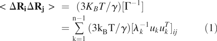where Γ is the Kirchhoff matrix of contacts, γ is the Hookean force constant between interacting sites, λ _k is the eigenvalue, and u _k is the eigenvector associated with the kth mode of motion. When i = j, Equation 1 describes the autocorrelation of the fluctuations, i.e., the mean-square fluctuations.

Equation 1 allows description of the fluctuations as a linear combination of a series of modes from slowest to fastest. The fluctuations in the slowest modes usually describe the global and most cooperative motions associated with biologically relevant functions (Bahar et al. 1997, 1998), whereas the fluctuations in the fast modes describe the high frequency local fluctuations. The residues contributing to the high frequency fluctuations are generally indispensable residues for stability and function (Bahar et al. 1998; Demirel et al. 1998).

In the present analysis, the high frequency end of the spectrum is of interest. The distribution of the fluctuations in an average of a number of fast modes (Haliloglu et al. 2005) is used to identify the high frequency vibrating (HFV) residues. Although the high frequency end of the spectrum is usually viewed as “uninteresting” in normal mode analysis, the peaks in the fastest GNM modes identify the residues that maintain structural integrity (Demirel et al. 1998). Within the scope of the energy landscape in mode space, the steepness of wells that have the same depth differ from one mode to the other. Modes with larger λ _i values characterized by steeper energy walls are more localized. The fluctuations related to these modes are accompanied by a larger decrease in entropy. Thus, the residues involved in fastest modes are referred to as kinetically hot residues. The resistance to conformational changes implies their importance in maintaining the structure. Previous studies have shown that these residues correlate with experimentally determined folding nuclei (Bahar et al. 1998; Demirel et al. 1998; Rader and Bahar 2004; Rader et al. 2004) as well as associate with the structurally conserved residues considered as binding hotspots at the interfaces (Haliloglu et al. 2005).

The algorithm for binding site prediction: HFV residue clusters and surface patches

An automated method is proposed and tested for its potency in determining putative binding regions. The algorithm is as follows:

1. The HFV residues are determined from the distribution of the fluctuations in the fastest modes of dynamics by GNM. These residues have a tendency to cluster in space. Here, we use a simple clustering algorithm (Haliloglu et al. 2005), which clusters the HFV residues in the structure based on their distances to each other. The algorithm yields a set of HFV residue clusters of varying sizes for a given structure.

2. The surface residues are identified by ACCESS (Lee and Richards 1971). The surface area for each residue is calculated and compared with the residue in Gly-X-Gly (Chothia 1975). Here, a residue is exposed if its accessible surface area (ASA) is >20% of its ASA in an extended conformation.

3. The surface residues are ranked according to their proximity to a group of HFV residues. This is based on our previous work (Haliloglu et al. 2005), which suggested that the binding residues (binding hotspots) are enriched by nearby HFV residues as compared with the rest of the surface residues. The average distance of the nearest 12 HFV sites, α-carbon positions, or side chain centroids to each surface residue is calculated. If this distance is <7.5 Å, this surface residue is considered as a candidate residue to be associated with an interface and is collected into a pool.

4. The surface residues collected in the pool (step 3) are clustered as in step 1 to determine surface patches that may overlap an interface region. Thus, a surface patch is a clustered set of surface residues that are under a distance threshold from an HFV site. A patch does not have a minimum size. A single residue can also constitute a patch.

The output of the algorithm (steps 1–4) is clusters of HFV residues and surface patches that are the patches of surface residues found to reside close to HFV sites. The association of both HFV clusters and surface patches with the interface regions is searched. The interface residues are defined with a criterion used in the original data sets, explained here in the section “Data sets”.

Results and Discussion

The proposed methodology was applied to the Benchmark Set and Cluster Set data sets, as follows:

Benchmark Set

The Benchmark Set includes protein–protein complex structures both in the bound and unbound states. First, we present detailed comparisons of the positions of the HFV residues with respect to the interface and the rest of the surface residues for two structures. Next, the positions of HFV residues, with respect to the interface residues, are analyzed for all of the structures in the data set, and the significance of the HFV residues at/near interfaces are assessed against the randomly distributed HFV residues. We proceed to a detailed analysis of subsets in the data set. Finally, we estimate the success of the prediction of the interface regions by the surface-patch residues identified through their proximity to the HFV residues.

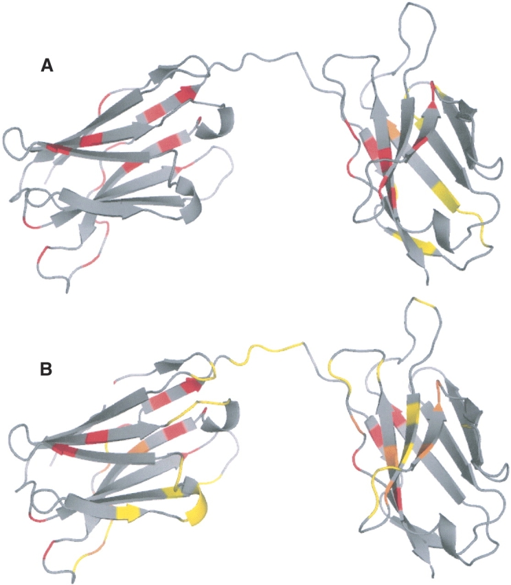
In Figure 1A, the distribution of the fluctuations in the fastest modes of dynamics is displayed for both the unbound (PDB code 1TBGAE) and bound (PDB code 1GOT) forms of Transducin Gt-β-γ, where the bound form is with Transducin Gt-α, Gi-α. The RMSD between the bound and unbound states is 1.05 Å (2.45 Å on the interface residues). The positions of the HFV residues do not show significant differences between the two states and correlate well with the positions of interface residues. For the unbound form, there are 34 identified HFV residues (of 338) clustered into four groups, three of which are located within 5 Å from the interface, while the fourth cluster of only one residue is located 12 Å away from the interface. There are three surface patches of 14 residues identified from their proximity to these HFV residues. Two of these surface patches comprise residues that overlap the interface residues, and the third patch of only one residue is 3.8 Å away from the interface. Figure 1B provides an example of another case: Barnase has 0.48 Å (0.47 Å on interface residues) RMSD between its unbound (PDB code 1A2P) and bound (PDB code 1BRS; Barstar) forms. Here, only one cluster of 17 HFV residues located 4.2 Å away from the interface is identified. One of the two surface patches of nine residues resides within an average distance of 0.7 Å from the interface. The second patch of one residue is 6 Å away from the interface. The HFV and the surface patch residues are presented on the ribbon diagrams (B1 and B2, respectively). As a further example, we refer to our recent work (Haliloglu et al. 2005), where the fluctuations of residues in fastest mode dynamics of gluthathione S-transferase between the bound and unbound states, differing by 8 Å RMSD, displayed a very similar behavior and are highly correlated with the interface residues. The observations here suggest that, in general, it is possible to deduce the relevant information from the unbound forms. HFV residues are mostly located near interface residues and in the core of the structure. Surface residues that overlap or are proximate to the HFV residues have a high propensity to be interface residues.

Figure 1.

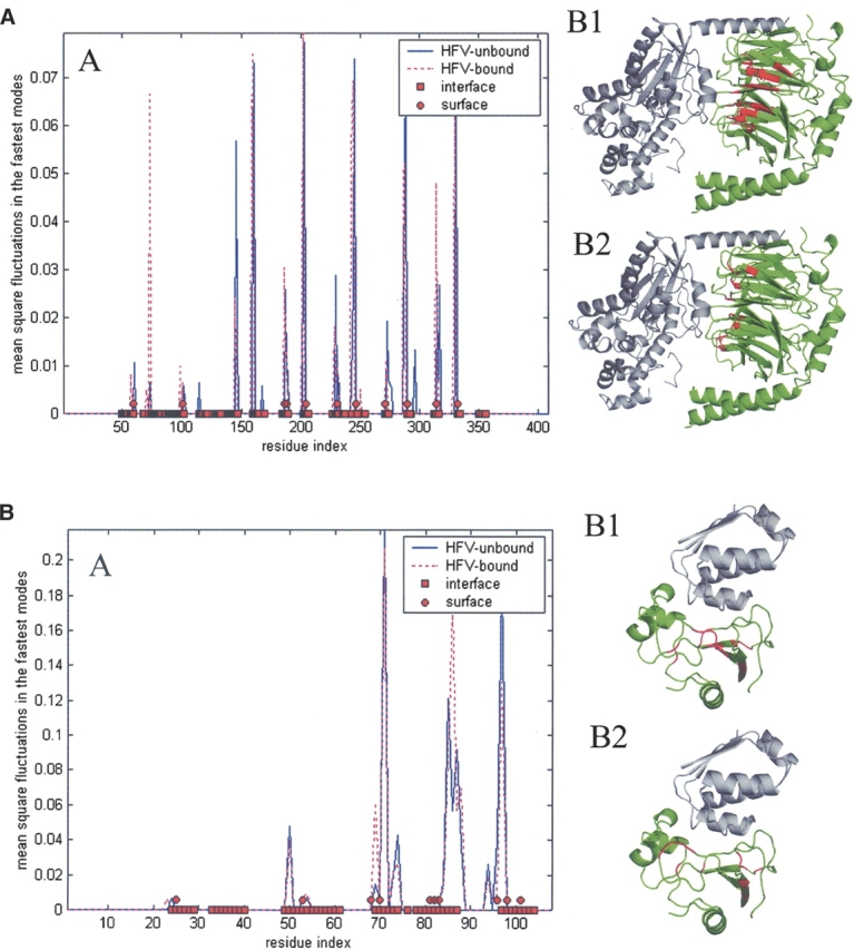
 (A) The distribution of fluctuations in the fastest modes of dynamics of Transducin Gt-β-γ, for both unbound (1TBGAE) and bound (in complex with Transducin Gt-α, Gi-α chimera [1GOT]) states (graph A). The structure is shown (green) with its ligand (gray) (B1,B2). The HFV residues and surface patch residues determined from the unbound state are shown in red (B1 and B2, respectively). Red squares and circles display interface and surface patch residues. (B) The distributions of fluctuations in the fastest modes of dynamics for Barnase both in unbound (1A2P) and bound to barstar (1BRS) states (graph A). The corresponding 3D-structure is shown on the right (B1,B2), with a similar description as in A.

Figure 2A displays the average number of the HFV residues by GNM versus by random sampling that are within 7.5 Å distance to an interface residue for the 110 structures in the Benchmark Set. For 79 structures among the 110, there is an enhanced packing close to the interface residues as reflected by the weight of the HFV residues by GNM over those by random sampling. The 25% of the cases displayed in Figure 2A, which do not show enrichment in HFV residues close to the interface, are observed to comprise mostly antigens and antibodies. Figure 2, B and C, displays the behavior of interface residues only for the structures in the subset of Antigen–Antibody and only for the structures in the subset of Enzyme–Inhibitor, respectively. The interface is more enriched by the HFV residues for 19 structures out of 34 and for 18 structures out of 21 in comparison with the random counterparts for the respective subsets. Figure 2D displays the density difference of the HFV residues around the interface and the rest of the surface. For 16 out of the 21 structures, the interface residues are more enriched with HFV residues compared with the rest of the surface residues. Thus, as can be observed, the algorithm can locate the binding regions in enzymes/inhibitors, but comparatively fails in antigens/antibodies. This apparently reflects a topological property of these structures (Alberts et al. 1994). Structural investigations have indicated that the antigen–antibody complexes display a less densely packed organization when compared with other protein structures (Neuvirth et al. 2004). Enzymes typically have clefts in their binding sites, and thus it is expected that they will be more densely packed and enriched in high frequency vibrating residues.

Figure 2.

 The number of HFV residues by GNM (X-axis) and by random sampling of HFV residues (Y-axis) per interface residue within 7.5 Å from the interface for the Benchmark Set (A) and for the subsets of Antigen–Antibody (B) and Enzyme (C). Interface residues of 79 structures out of 110, 19 structures out of 34, and 18 structures out of 21 are more enriched with the HFV residues, in comparison with the random occurrence of the HFV residues for the respective sets. (D) Comparison of the number of HFV residues located within 7.5 Å of the interface per interface residue with that of the rest of surface residues (Y-axis) for the subset of Enzyme. For 16 structures out of 21, the interface residues are more enriched with HFV residues compared to the rest of surface residues.

Table 1 gives the average numbers of the HFV residues in contact (maximum contact distance is 7.5 Å) with interface and non-interface residues for the Benchmark Set and for the subsets of Enzyme, Antigen–Antibody, Others, and Difficult. Here, the average is taken over the total number of structures in each set. The variances for each data set are given in parentheses. The results point out that a noticeable difference between the interface and the rest of the surface residues exist for the subset of Enzyme. As for the subset of Difficult, which shows large conformational changes upon binding, a difference is also observed in densities of the HFV residues favoring the interface with respect to the rest of the surface residues. For the subset of Antigen–Antibody, it is hard to see any difference that differentiates the interface and the rest of the surface. The HFV residues favor non-interface residues in the subset of Others. The t-tests applied to each subset indicate that for the subset of Enzyme, the difference in preference of HFV residues toward the interface and rest of the surface is statistically significant within 95% confidence interval. For the rest of the subsets, the differences were found to be statistically insignificant. For the entire benchmark, as it includes particularly the subset of Antigen–Antibody, the difference between surface and interface residues with respect to HFV residues is not significant.

Table 1.

 The average number of HFV residues that the interface and non-interface (rest of the surface) residues are in contact with (maximum contact distance is 7.5 Å) for the Benchmark Set and the subsets of Enzyme, Antigen–Antibody, Others, and Difficult

In the analysis above, individual HFV residues were analyzed. Nevertheless, the HFV residues cluster and the clusters can further contribute to the identification of the surface patches. The average number of the HFV residue clusters and surface patches were calculated as 2.9 and 2.7 with average sizes of 9.3 and 4.9 residues, respectively. The average numbers of HFV residue clusters and surface patches for the random distribution of the HFV residues were calculated as 6.9 and 2.8, with average sizes of 4 and 3.5 residues, respectively. The average sizes of the residue clusters and the surface patches nearest the interface were calculated as 8.6 and 5.1 residues, respectively, with average distances of 2.1 Å and 2.4 Å to the interface. The nearest HFV residue and surface cluster sizes for the random sampling are 3.0 and 3.8, respectively. The numbers above reflect the clustering tendency for the HFV residues and for the surface patch residues located nearby.

Table 2 displays the percentage of the structures that have at least one cluster of HFV residues near the interface and at least one surface patch located within different frame sizes. The results indicate that for 75% of the test cases there is at least one cluster of HFV residues within 7 Å distance from the interface. The corresponding value for the surface patches located close to the HFV residues is 88%. Additional analysis on HFV clusters of the Benchmark Set indicates that for 41.8% of the test cases, there was at least one HFV cluster which had no residue within 7 Å of the interface. For 40% of these cases, the identified cluster was less than five residues. On the other hand, previous studies (Bahar et al. 1998; Demirel et al. 1998) implied that the HFV residues were also associated with the active sites or functionally important residues of the proteins, which may be located on a different site from the binding interface. There might also be other binding sites in the structure apart from the one analyzed.

Table 2.

 The percentage of the structures that have at least one HFV residue cluster (second column) and surface patch (third column) within different frame sizes (first column), for the Benchmark Set

These values indicate that both the location of the HFV residues and the surface patches determined from these HFV residues can be associated with putative binding sites, and as such, can be useful for their prediction.

Cluster Set

For the Benchmark Set above, the analysis was carried out mostly on the unbound forms and includes specific types of structures. Here, the algorithm is tested on another, more-diversified set of structures: a database of protein–protein interfaces in the Cluster Set, for which only the three-dimensional structures of the bound forms are available. This is on the premise that there is no significant difference between the bound and the unbound states with respect to the position of the HFV residues.

The significance of the preference of the HFV residues to locate close to interface regions is assessed against the randomly distributed HFV residues for the structures in the Cluster Set. The results indicate that the HFV residues cluster, and in general, the largest clusters are associated with the interface regions. In general, since HFV residue clusters are frequently associated with higher packing density, they are located in the core of the structure. Hence, the surface patches identified due to their proximity to the HFV residues would also correlate well with interface regions as shown below with specific examples.

Figure 3A displays the average percentages of the HFV residues by GNM located within varying distance intervals (e.g., “zero” interval is defined as the distance ≥0 and <2 Å) from the interface in comparison with that of the randomly distributed HFV residues. Interface residues within a layer of 8 Å are 27% enriched by HFV residues; i.e., the number of HFV residues that are in the 8 Å vicinity of an interface is on average 27% larger than that for random occurrence. A total of 61% of the HFV residues are observed to be located within 8 Å of the interface. This percentage is 44 for the random counterpart. Figure 3B displays the number of HFV residues by GNM within 7.5 Å of each interface residue (X-axis) in comparison with the corresponding values by HFV residues distributed randomly (Y-axis) for each structure in the Cluster Set. For 34 cases out of 50, the number of HFV residues that are closer than 7.5 Å from the interface is greater than that of the random case.

Figure 3.

 (A) The percentage distribution of the minimum distances of HFV residues (the shortest distance; either α-C or side chain centroid) by GNM to the interface in comparison with that of the same number of HFV residues sampled randomly. The distribution is averaged over 50 structures from the Cluster Set. (B) The number of HFV residues per interface residue within 7.5 Å by GNM (X-axis) and by the random sampling (Y-axis) for the structures in the Cluster Set. For 34 structures out of 50, the interface residues have a higher number of HFV residues nearby than predicted by the randomly distributed HFV residues.

HFV residues cluster in space. The number of HFV residue clusters averaged over the structures in the Cluster Set is 3.3, with an average cluster size of 9.4 residues. The average size of the largest HFV residue cluster is 21.5, with an average distance of 10 Å to the interface. Seventy percent of the largest clusters are located within 8 Å of the interface residues. In a random distribution of HFV residues, the average number of HFV clusters is 7.6, with an average size of 4.0 residues, and the average size of the largest HFV clusters is calculated as 11, with an average distance of 12.4 Å from the interface.

These results and the observation from our previous work (Haliloglu et al. 2005) indicate that interface residues are enriched by nearby HFV residues both in comparison with the random distribution of the HFV residues and with respect to the rest of surface residues. This suggests that the identification of surface patches based on a group of HFV residues nearby is likely to increase the success of the prediction. To test this scheme, as in the Benchmark Set, surface patches for the Cluster Set were identified by calculating the average distance of any surface residue to the nearest 12 sites belonging to α-carbons or side chain centroids of the HFV residues (Haliloglu et al. 2005). Thus, groups of surface residues that are enriched in HFV residues are registered as likely to overlap with binding regions. The average number of surface patches is 3.6, with an average size of 4.7 residues. In a random distribution of HFV residues, less surface residues and smaller patch sizes that fit the criteria could be mapped (3.2 and 2.6, respectively).

Table 3 displays the percentage of the structures that have the nearest HFV residue clusters and surface patches to the interface residues within the specified distances. The results indicate that for 70% of the cases there is at least one cluster of HFV residues, and for 84% of the cases there is at least one surface patch located within 7 Å distance from the interface. The hot spots/HFV residues are mostly buried. Thus, surface patches identified in close proximity to the HFV residues are more likely to be located nearer the binding sites when compared with the HFV clusters.

Table 3.

 The percentage of the structures that have at least one HFV residue cluster (second column) and surface patch (third column) within different frame sizes (first column), for the Cluster Set

Below, we illustrate three cases. Figure 4 presents the results of the analysis on Subtilisin novo proteinase (PDB code 2SNI). This structure has 275 residues. Forty-one HFV residues are identified (Fig. 4A), grouping into four HFV residue clusters. The largest cluster has 34 residues. The HFV residues lead to nine surface residues that are grouped into three surface patches. One of the patches overlaps the main data set interface (Fig. 4C). Another patch overlaps a metal-binding site (Fig. 4D). Close to the main interface there is another metal-binding site (Fig. 4D), which partially overlaps the main interface. Figure 4B shows that residues belonging to the first two surface patches are conserved or located near conserved residues. The third surface patch may be a false prediction.

Figure 4.

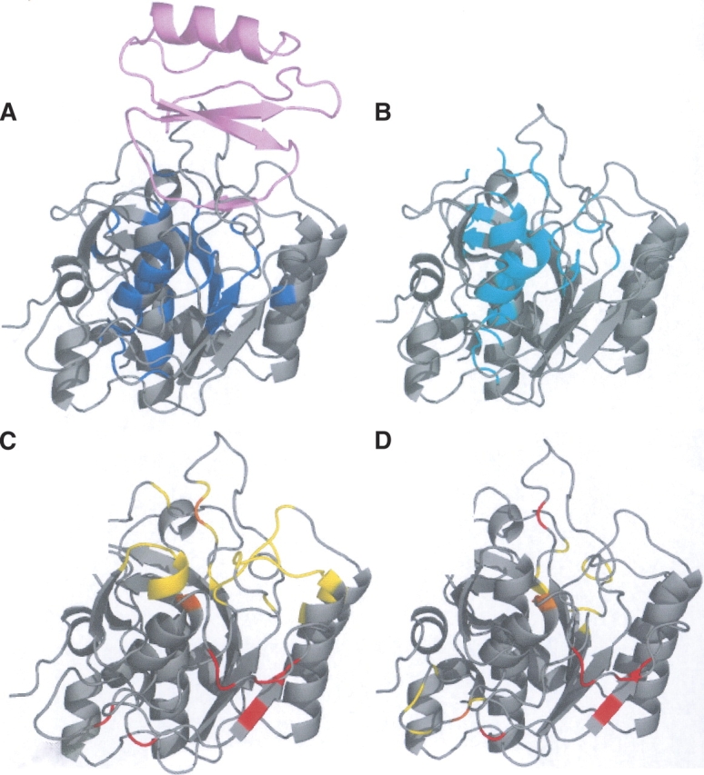
 Subtilisin novo proteinase (2SNI) with 275 residues. (A) Forty-one HFV residues that are grouped into four clusters are colored blue, displayed with its partner structure (pink) in the complex. (B) The conserved residues are colored cyan. (C) The main interface is colored yellow; the three surface patches of nine residues are colored red and the overlap is colored orange. (D) Metal binding sites are colored yellow, surface patches are red, and the overlap is orange. The overlap is between surface path residues and interface residues.

As another representative case, the results of the analysis for the complexed variable domain from λ-6 type immunoglobulin Jto (PDB code 1CD0A) light chain are presented in Figure 5. A total of 17 HFV residues are identified grouped into one cluster (blue in Fig. 5A). Two surface patches are determined here (Fig. 5C). The larger surface patch with eight residues successfully locates the binding region. The small patch (with one residue) does not overlap any known interface. There are no additional binding sites known (available) for this structure. However, conservation data (Fig. 5B) indicate that the single residue surface patch is one of the highly conserved residues, suggesting some functional importance.

Figure 5.

 Jto, a variable domain from λ-6 type immunoglobulin light chain with 111 residues (1CD0). (A) Seventeen HFV residues are colored blue, displayed in complex. (B) The conserved residues are in cyan. (C) The main binding site is colored yellow, the surface patches composed of nine residues in two patches with eight and one residues are colored red, and the intersection is colored orange.

Another example is a trimer Yjgf protein (PDB code 1QU9A) with 126 residues (Fig. 6). The HFV residues (Fig. 6A), the highly conserved residues (Fig. 6B), the surface patch residues, and the two different binding interface residues (Fig. 6C,D) are displayed. A total of 21 HFV residues are in three clusters, where one is of 19 residues. The main and the second binding interfaces are presented in Figure 6, C and D, respectively, in comparison with the two identified surface patches. The larger surface patch is composed of 10 residues and is located at an average distance of 5 Å from the interface, successfully locating the interface residues. The smaller surface patch of two residues is located 12 Å away from the interface.

Figure 6.

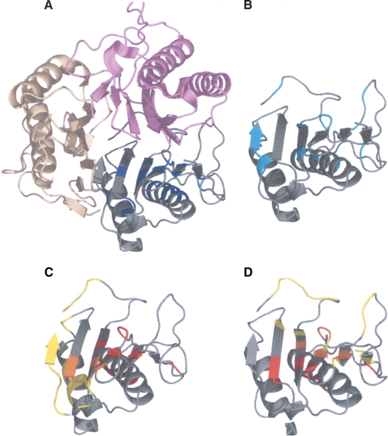
 Yjgf protein (1QU9) with 126 residues. Twenty-one HFV residues are determined, 19 are grouped into one cluster. The surface patches determined are composed of 12 residues clustered into groups of 10 and 12. (A) The HFV residues are colored blue; the complex partners are in two different shades of pink. (B) The conserved residues are in cyan. (C) The main binding site is in yellow, the surface patches are colored red, and the intersection colored orange. (D) The second binding site is colored yellow, the surface patches colored red, and the intersection is colored orange.

There are eight outlier structures, with no surface patch within 7.5 Å from the binding interface: 1bjj A, 1fj1D, 1fj1E, 1lmk A, 1AS4A, 1aw1A, 1jixC, and 1fytD (see Supplemental Table A.2). As an example, immunoglobulin (1LMKA) is displayed in Figure 7. A total of 39 HFV residues out of 238 residues are identified in four clusters. The surface patches identified from these HFV residues are composed of 26 residues in six surface patches. The interface residues for which the analysis is carried out are shown in yellow, the predicted surface patches are red and the overlapping residues are orange. This figure indicates that the surface patches identified here lead to a false prediction. However, a second binding interface is shown for the same protein (Fig. 7B) overlapping HFV residues. Thus, again, immunoglobulins appear not to be amenable to prediction based on this strategy.

Figure 7.

 One of the outliers,immunoglobulin (1LMK). A total of 39 residues out of 238 are identified as HFF residues, which clustered into four groups. The surface patches identified from the HFF residues are composed of 26 residues clustered into six patches. In A and B, the original and a second binding sites are displayed, respectively. The interface residues are colored yellow, the surface patches are colored red, and the intersection residues are colored orange.

The analysis described here suggests that larger HFV residue clusters are more likely to locate near the interface region, and surface patches successfully locate some interface residues. The additional consideration of conservation data assists in filtering out false predictions.

In the analysis carried out in the present study, each overlap is considered to be equally significant. Devising a clear measure of overlap significance with respect to the sizes of clusters or patches and interfaces and for different sets of proteins is not straightforward. With the low-resolution presentation of the structure, which lacks side chain information and describes only backbone centers, the identified patches from HFV clusters provide only approximate locations for the interfaces. Based on our previous work (Haliloglu et al. 2005), sites associated with HFV clusters correspond to binding hotspots at the interfaces. The association of the HFV clusters with the interface residues is thus mainly due to the association with possible hotspots at the interfaces and not with all of the interface residues.

In this respect, the lack of specificity of amino acid types and sizes due to the low resolution of the model might affect the association between HFV clusters and interfaces. In particular, the preferences of certain types of amino acids at the interfaces are known (Ma et al. 2003). Here, the amino acid types might be included indirectly if certain types would induce specific geometrical arrangement in the packing environment. The GNM with the more computationally expensive calculations on an atomistic description of the residues might improve this association to a certain extent. Nevertheless, although there is an intimate connection between sequence, structure, and dynamics, an ideal description of the interface may require explicit consideration of some properties of interface residues in the prediction. Overall, inspection of the results leads us to suggest that concave binding interfaces (typically those of enzyme binding sites), are enriched by the HFV residues.

Conclusions

Binding site prediction is one of the bottlenecks for prediction of protein function, drug design, and for putting proteins together in Systems Biology. Many experimental and computational methods have been developed to predict interface residues of proteins. Experimental methods mostly address the stability and energetics of binding, while computational methods also consider distinguishing properties of the interfaces versus the rest of the surface, such as composition, architecture, and conservation. Most of the methods lack information on the dynamics of proteins, although proteins are not rigid objects, and their surfaces are plastic.

Interface regions often contain cavities. The packing density increases at the cavities leading to an environment where residues are expected to display high frequency fluctuations. Analysis of the fluctuation behavior of the residues in their native state dynamics by the Gaussian Network Model confirms that high frequency fluctuating residues are enriched in the vicinity of the interface as compared with the rest of the surface. Our analysis also indicates that the HFV residues are invariant between the unbound and bound forms, suggesting a pre-organization of the binding sites, and further indicating that such a strategy is applicable to the unliganded state, the state that is of interest for the purpose of prediction. Thus, high frequency fluctuating residues can be used for locating surface patches that may constitute binding sites. Here, the overlap of the HFV residue clusters and surface patches with interfaces was studied in the two data sets, the Benchmark Set and the Cluster Set.

The present approach is a plausible strategy for detecting binding regions based on a single structure. Since it relates to local packing density, it is expected that interfaces with more invaginations and cavities will be better predicted by high frequency vibrating residues. Thus, we expect that the association of HFV residues with the interfaces holds true mostly for enzymes, where the effect is the strongest. Nevertheless, if a binding region has invaginations and cavities (as in some of the antigen/antibodies and in cases in the Cluster data set) we expect that it would be detected there too. The practical utility of the proposed method will be enhanced by additional available tools, such as conservation. This method may further provide insight into the relationship between structure, dynamics, and function, since the HFV residues displaying restricted fluctuations should overlap the minima of the slowest mode shapes, which describe the most cooperative modes. Finally, since these residues reflect regions with high packing density, they are expected to contribute to the free energy of the binding. As we have already shown, they correlate with energy hot spots or are in their vicinity (Haliloglu et al. 2005).

References

- Alberts, B., Bray, D., Lewis, J., Raff, M., Roberts, K., Watson, J.D. In Molecular biology of the cell. .1994. Garland Publishing, New York.
- Bahar, I., Atilgan, A., Erman, B. 1997. Direct evaluation of thermal fluctuations in proteins using a single parameter harmonic potential. Fold. Des. 2: 173–181. [DOI] [PubMed] [Google Scholar]
- Bahar, I., Atilgan, A.R., Demirel, M.C., Erman, B. 1998. Vibrational dynamics of proteins: Significance of slow and fast modes in relation to function and stability. Phys. Rev. Lett. 80: 2733–2736. [Google Scholar]
- Bartlett, G.J., Porter, T.P., Borkakoti, N., Thornton, J.M. 2002. Analysis of catalytic residues in enzyme active sites. J. Mol. Biol. 324: 105–121. [DOI] [PubMed] [Google Scholar]
- Brinda, K.V., Kannan, N., Vishveshwara, S. 2002. Analysis of homodimeric protein interfaces by graph-spectral methods. Protein Eng. 15: 265–277. [DOI] [PubMed] [Google Scholar]
- Casari, G., Sander, C., Valencia, A. 1995. A method to predict functional residues in proteins. Nat. Struct. Biol. 2: 171–178. [DOI] [PubMed] [Google Scholar]
- Cheng, R., Mintseris, J., Janin, J., Weng, Z. 2003. A protein–protein docking benchmark. Proteins 52: 88–91. [DOI] [PubMed] [Google Scholar]
- Chothia,, C. 1975. Nature of accessible and buried surfaces in proteins. J. Mol. Biol. 105: 1–14. [DOI] [PubMed] [Google Scholar]
- Clackson, T. and Wells, J.A. 1995. A hot spot of binding energy in a hormone-receptor interface. Science 267: 383–386. [DOI] [PubMed] [Google Scholar]
- Enzyme evolution explained (sort of).Dean, A.M. and Golding, G.B. Pacific Symposium on Biocomputing. 2000. 6–17. [DOI] [PubMed]
- DeLano, W.L. 2002. Unraveling hot spots in binding interfaces: Progress and challenges. Curr. Opin. Struct. Biol. 12: 14–20. [DOI] [PubMed] [Google Scholar]
- Demirel, M.C., Atilgan, A.R., Jernigan, R.L., Erman, B., Bahar, I. 1998. Identification of kinetically hot residues in proteins. Protein Sci. 7: 2522–2532. [DOI] [PMC free article] [PubMed] [Google Scholar]
- Dominguez, C., Boelens, R., Bonvin, A.M. 2003. HADDOCK: A protein–protein docking approach based on biochemical or biophysical information. J. Am. Chem. Soc. 125: 1731–1737. [DOI] [PubMed] [Google Scholar]
- Fariselli, P., Pazos, F., Valencia, A., Haliloglu, T. 2002. Prediction of protein–protein interaction sites in heterocomplexes with neural networks. Eur. J. Biochem. 269: 1356–1361. [DOI] [PubMed] [Google Scholar]
- Fernandez-Recio, J., Totrov, M., Skorodumov, C., Abagyan, R. 2005. Optimal docking area: A new method for predicting protein–protein interaction sites. Proteins 58: 134–143. [DOI] [PubMed] [Google Scholar]
- Glaser, F., Pupko, T., Paz, I., Bell, R.E., Bechor-Shental, D., Martz, E., Ben-Tal, N. 2003. ConSurf: Identification of functional regions in proteins by surface-mapping of phylogenetic information. Bioinformatics 19: 163–164. [DOI] [PubMed] [Google Scholar]
- Haliloglu, T., Bahar, I., Erman, B. 1997. Gaussian dynamics of folded proteins. Phys. Rev. Lett. 79: 3090–3093. [Google Scholar]
- Haliloglu, T., Keskin, O., Ma, B., Nussinov, R. 2005. How similar are protein folding and protein binding nuclei? Examination of vibrational motions of energy hotspots and conserved residues. Biophys. J. 88: 1552–1559. [DOI] [PMC free article] [PubMed] [Google Scholar]
- Huan-Xiang, Z. and Yibing, S. 2001. Prediction of protein interaction sites from sequence profile and residue neighbor. Proteins 44: 336–343. [DOI] [PubMed] [Google Scholar]
- Jambon, M., Imberty, A., Deleage, G., Geourjon, C. 2003. A new bioinformatic approach to detect common 3D sites in protein structures. Proteins 52: 137–145. [DOI] [PubMed] [Google Scholar]
- Jones, S. and Thornton, J.M. 1997. Prediciton of protein–protein interaction sites using patch analysis. J. Mol. Biol. 272: 133–143. [DOI] [PubMed] [Google Scholar]
- Keskin, O., Tsai, C.J., Wolfson, H., Nussinov, R. 2004. A new, structurally nonredundant, diverse data set of protein–protein interfaces and its implications. Protein Sci. 13: 1043–1055. [DOI] [PMC free article] [PubMed] [Google Scholar]
- Keskin, O., Ma, B., Nussinov, R. 2005. Hot regions in protein–protein interactions: The organization and contribution of structurally conserved hot spot residues. J. Mol. Biol. 345: 1281–1294. [DOI] [PubMed] [Google Scholar]
- Kini, R.M. and Evans, H.J. 1995. A hypothetical structural role for proline residues in the flanking segments of protein–protein interaction sites. Biochem. Biophys. Res. Commun. 212: 1115–1124. [DOI] [PubMed] [Google Scholar]
- Kinoshita, K. and Nakamura, H. 2005. Identification of the ligand binding sites on the molecular surface of proteins. Protein Sci. 14: 711–718. [DOI] [PMC free article] [PubMed] [Google Scholar]
- Kortemme, T. and Baker, D. 2002. A simple physical model for binding energy hot spots in protein–protein complexes. Proc. Natl. Acad. Sci. 99: 14116–14121. [DOI] [PMC free article] [PubMed] [Google Scholar]
- Landgraf, R., Xenarios, I., Eisenberg, D. 2001. Three-dimensional cluster analysis identifies interfaces and functional residue clusters in proteins. J. Mol. Biol. 307: 1487–1502. [DOI] [PubMed] [Google Scholar]
- Lee, B. and Richards, F.M. 1971. The interpretation of protein structures estimation of static accessibility. J. Mol. Biol. 55: 379–400. [DOI] [PubMed] [Google Scholar]
- Li, X., Keskin, O., Ma, B., Nussinov, R., Liang, J. 2004. Protein–protein interactions: Hotspots and structurally conserved residues often locate in the complemented pockets that pre-organized in the unbound states: Implications for docking. J. Mol. Biol. 344: 781–795. [DOI] [PubMed] [Google Scholar]
- Lichtarge, O., Bourne, H.R., Cohen, F.E. 1996. An evolutionary trace method defines binding surfaces common to protein families. J. Mol. Biol. 257: 342–358. [DOI] [PubMed] [Google Scholar]
- Lim, D., Park, H.U., DeCastro, L., Kang, S., Lee, H.S., Jensen, S., Lee, K.J., Strynadka, N.C. 2001. Crystal structure and kinetic analysis of β-lactamase inhibitor protein-II in complex with TEM-1 β-lactamase. Nat. Struct. Biol. 8: 848–852. [DOI] [PubMed] [Google Scholar]
- Livingston, C.D. and Barton, G.J. 1993. Protein sequence alignments: A strategy for the hierarchical analysis of residue conservation. Comp. Appl. Biosci. 6: 645–656. [DOI] [PubMed] [Google Scholar]
- Luque, I. and Freire, E. 2000. Structural stability of binding sites: Consequences for binding affinity and allosteric effects. Proteins 4: 63–71. [DOI] [PubMed] [Google Scholar]
- Ma, B., Elkayam, T., Wolfson, H., Nussinov, R. 2003. Protein–protein interactions: Structurally conserved residues distinguish between binding sites and exposed protein surfaces. Proc. Natl. Acad. Sci. 100: 5772–5777. [DOI] [PMC free article] [PubMed] [Google Scholar]
- Madabushi, S., Yao, H., Marsh, M., Kristensen, D.M., Philippi, A., Sowa, M.E., Lichtarge, O. 2002. Structural clusters of evolutionary trace residues are statistically significant and common in proteins. J. Mol. Biol. 316: 139–154. [DOI] [PubMed] [Google Scholar]
- Marti-Renom, M.A., Stuart, A.C., Fiser, A., Sanchez, R., Melo, F., Sali, A. 2000. Comparative protein structure modeling of genes and genomes. Annu. Rev. Biophys. Biomol. Struct. 29: 291–325. [DOI] [PubMed] [Google Scholar]
- Neuvirth, H., Raz, R., Scheiber, G. 2004. ProMate: A structure based prediction program to identify the location of protein–protein binding sites. J. Mol. Biol. 338: 181–199. [DOI] [PubMed] [Google Scholar]
- Nimrod, G., Glaser, F., Steinberg, D., Ben-Tal, N., Pupko, T. 2005. In silico identification of functional regions in proteins. Bioinformatics 21 (Suppl 1): i328–i337. [DOI] [PubMed] [Google Scholar]
- Pazos, F., Helmer-Citterich, M., Ausiello, G., Valencia, A. 1997. Correlated mutations contain information about protein–protein interaction. J. Mol. Biol. 271: 511–523. [DOI] [PubMed] [Google Scholar]
- Rader, A.J. and Bahar, I. 2004. Folding core predictions from network models of proteins. Polymer 45: 659–668. [Google Scholar]
- Rader, A.J., Anderson, G., Isin, B., Khorana, H.G., Bahar, I., Klein-Seetharaman, J. 2004. Identification of core amino acids stabilizing rhodopsin. Proc. Natl. Acad. Sci. 101: 7246–7251. [DOI] [PMC free article] [PubMed] [Google Scholar]
- Sandak, B., Wolfson, H., Nussinov, R. 1998. Flexible docking allowing induced fit in proteins: Insights from an open to closed conformational isomers. Proteins 32: 159–174. [PubMed] [Google Scholar]
- Smith, G.R. and Sternberg, M.J.E. 2005. The relationship between the flexibility of proteins and conformational states on forming protein–protein complexes with an application to protein–protein docking. J. Mol. Biol. 347: 1077–1101. [DOI] [PubMed] [Google Scholar]
- Szilagyi, A., Grimm, V., Arakaki, A.K., Skolnick, J. 2005. Prediction of physical protein–protein interactions. Phys. Biol. 2: 1–16. [DOI] [PubMed] [Google Scholar]
- Todd, A.E., Orengo, C.A., Thornton, J.M. 2001. Evolution of funciton in protein superfamilies, from a structural perspective. J. Mol. Biol. 307: 1113–1143. [DOI] [PubMed] [Google Scholar]
- Wagnikar, P.P., Tendulka, A.V., Ramya, S., Mail, D.N., Sarawagi, S. 2003. Functional sites in protein families uncovered via an objective and automated graph theoretic approach. J. Mol. Biol. 326: 955–978. [DOI] [PubMed] [Google Scholar]
- Yang, L.W. and Bahar, I. 2005. Coupling between catalytic site and collective dynamics: A requirement for mechanochemical activity of enzymes. Structure 13: 893–904. [DOI] [PMC free article] [PubMed] [Google Scholar]
- Yao, H., Kristensen, D.M., Mihalek, I., Sowa, M.E., Shaw, C., Kimmel, M., Kavraki, L., Lichtarge, O. 2003. An accurate, sensitive and scalable method to identify functional sites in protein structures. J. Mol. Biol. 326: 255–261. [DOI] [PubMed] [Google Scholar]