Abstract
The major aim of tertiary structure prediction is to obtain protein models with the highest possible accuracy. Fold recognition, homology modeling, and de novo prediction methods typically use predicted secondary structures as input, and all of these methods may significantly benefit from more accurate secondary structure predictions. Although there are many different secondary structure prediction methods available in the literature, their cross-validated prediction accuracy is generally <80%. In order to increase the prediction accuracy, we developed a novel hybrid algorithm called Consensus Data Mining (CDM) that combines our two previous successful methods: (1) Fragment Database Mining (FDM), which exploits the Protein Data Bank structures, and (2) GOR V, which is based on information theory, Bayesian statistics, and multiple sequence alignments (MSA). In CDM, the target sequence is dissected into smaller fragments that are compared with fragments obtained from related sequences in the PDB. For fragments with a sequence identity above a certain sequence identity threshold, the FDM method is applied for the prediction. The remainder of the fragments are predicted by GOR V. The results of the CDM are provided as a function of the upper sequence identities of aligned fragments and the sequence identity threshold. We observe that the value 50% is the optimum sequence identity threshold, and that the accuracy of the CDM method measured by Q3 ranges from 67.5% to 93.2%, depending on the availability of known structural fragments with sufficiently high sequence identity. As the Protein Data Bank grows, it is anticipated that this consensus method will improve because it will rely more upon the structural fragments.
Keywords: secondary structure prediction, GOR, Fragment Database Mining, structural fragments, multiple sequence alignments, PSIPRED
Protein function is inherently correlated with structure. Most computational problems in protein science, such as protein docking (Camacho and Vajda 2002; Halperin et al. 2002; Smith and Sternberg 2002; Tovchigrechko et al. 2002), protein design (Mendes et al. 2002; Park et al. 2004; Vizcarra and Mayo 2005), binding/active site determination (Sen et al. 2004; Keskin et al. 2005; Szilagyi et al. 2005), and protein–protein interaction networks (Chaudhuri and Chant 2005), all rely on protein structure information of various types. In principle, combining most diverse information should yield the best results. The rapidly growing number of experimentally determined structures serves as a primary source of information. The number of known protein structures deposited in the Protein Data Bank (PDB) (Berman et al. 2000) is currently (August 2006) ∼38,000 (counting all, even highly homologous structures), a number that is significantly below the 233,000 or so protein sequences available in UniProtKB/Swiss-Prot database, and the 3,050,000 translations of EMBL nucleotide sequences collected in UniProtKB/TrEMBL database. Additionally, due to completion of many large-scale genome-sequencing projects, the number of known sequences grows continuously at an incredible rate.
Protein tertiary structure prediction from sequence is one of the most important problems in molecular biology. Recent significant advances in protein tertiary structure prediction using computational methods, measured by the Critical Assessment of Techniques for Protein Structure Prediction (CASP) experiments, may help reduce this large gap. These structure prediction methods can be broadly grouped into three categories: homology/comparative modeling, fold recognition/threading, and de novo (ab initio) modeling. Among these methods, homology modeling requires the highest sequence similarity to known structures from the PDB, while de novo modeling relies to a lesser extent on information from the sequences and from the structures of proteins in the PDB. Many tertiary structure prediction methods incorporate secondary structure prediction for improvement of the accuracy of their modeling, or to significantly reduce the sampling of conformational space that is required (Kolinski 2004; Solis and Rackovsky 2004; Kolinski and Bujnicki 2005).
Currently no secondary structure prediction techniques yield >80% accuracy in cross-validated predictions, measured by Q3 prediction accuracy (Rost 2001). For example, the most successful techniques based on neural networks, such as PHD (Rost 1996) and PSIPRED (Jones 1999), reported accuracies ∼76%. This limitation in prediction accuracy of secondary structures is subsequently transferred into many tertiary structure prediction methods, limiting their performance whenever such secondary structure predictions are used as the input to the structure prediction algorithm.
Secondary structure prediction is an active research area. Recently, support vector machines (Hua and Sun 2001; Nguyen and Rajapakse 2005), sequence-based two-level (Huang et al. 2005), and dihedral angle-based (Wood and Hirst 2005) neural network algorithms were successfully used with accuracies <80%. Neural networks were also applied for the cases where secondary structures are combined not only into three categories (helix, sheet, and coil), but also into seven categories in a more detailed representation (Lin et al. 2005).
Despite the variety of these prediction methods, the barrier of cross-validated 80% accuracy is still present and has not yet been overcome. Is there a structural explanation for this limit? In a recent, interesting work, Kihara (2005) pointed out the importance of long-range interactions on the formation of secondary structure. He argued that as long as secondary structure predictions are based on a sliding sequence window, the long-range effects, not only for β-sheets but even for helices, will be treated to a limited extent. A comparison of accuracies as a function of residue contact order (sequence separation between contacts) supports this argument, at least for some helical and coil fragments, and provides interesting implications for protein folding (Tsai and Nussinov 2005). However, the accuracies for some other helices with high-contact order were also low, suggesting that there might be other effects not taken into account in the present secondary structure prediction algorithms. Note that the incorporation of multiple sequence alignments into predictions implicitly introduces long-range effects since sequence conservation is guided by structural constraints; GOR V and now the present novel hybrid method both benefit from this inclusion.
In order to improve the accuracy of secondary structure predictions, we propose a new hybrid method, Consensus Data Mining (CDM), which combines our two previous successful secondary structure prediction methods: the recently developed Fragment Database Mining (FDM) (Cheng et al. 2005) and the latest version of the well known GOR algorithm, GOR V (Kloczkowski et al. 2002; Sen et al. 2005). The basic premise of CDM is that the combination of these two complementary methods can enhance the performance of secondary structure prediction by harnessing the distinct advantages that both methods offer. FDM exploits the availability of sequentially similar fragments in the PDB, which leads to the highly accurate (much better than GOR V) prediction of structure for such fragments, but such fragments are not available for many cases. On the other hand, GOR V predicts the secondary structure of less similar fragments fairly accurately, where usually the FDM method cannot find suitable structures.
Results
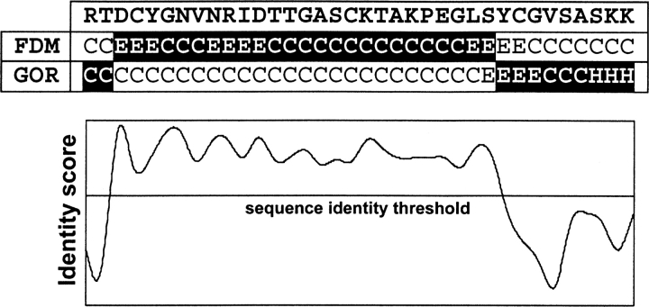
CDM exploits the strengths of two complementary methods, FDM and GOR V. As explained in detail in the Materials and Methods section, the CDM algorithm relies upon a single parameter (sequence identity threshold) to specify whether to apply FDM or GOR V prediction at a given site. The representation of the CDM method is shown in ▶, where the first row is a part of the query sequence, and the second and the third rows are the FDM and GOR V predictions. In order to decide which method is used for CDM, first an identity score map is generated for the fragment data. Depending on the sequence identity score, either FDM (if the site has a score higher than the sequence identity threshold) or GOR V is used for the CDM. The highlighted portions of ▶ specify which predictions are used in CDM.
Figure 1.
The graphical representation of the CDM method. For a given sequence fragment, the FDM and GOR V three-state predictions are calculated. Then, according to a sequence identity threshold (shown as a straight horizontal line), the regions with higher identity scores (above the line) predicted by FDM are selected, and the rest by GOR V. The final predictions are highlighted in black background.
The success of FDM depends largely upon the availability of similar fragments to the target sequence. In practice, however, the availability of similar sequences can vary significantly. In order to analyze the relationship between the performance of CDM and the sequence similarity of fragments, we have methodically excluded fragment alignments with sequence identities above a certain limit, and have called this limit the “upper sequence identity limit.” The upper sequence identity limit is not an additional parameter in the CDM method; these results demonstrate what the expected results would be in the absence of structural fragments having similarities above the sequence identity limit.
The performance of GOR V can also be improved with multiple sequence alignments: The GOR V method tested with the full jack-knife methodology yields an accuracy of 73.5%, when multiple sequence alignments (MSA) are included; otherwise, its accuracy is 67.5%.
One of the significant advantages of FDM is its applicability to various evolutionary problems because the algorithm does not rely exclusively on the sequences with the highest sequence similarity, but assigns weights to BLAST-aligned sequences that apparently capture divergent evolutionary relationships. As a result, CDM, which incorporates FDM, can be successfully used, even when there is a significant range of sequence similarities among the BLAST identified sequences.
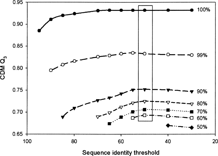
Although the availability of sequences with high similarity in the PDB essentially depends upon the target sequence, the question remains as to what the optimum value of the sequence identity threshold should be. To identify this optimal threshold, we applied the CDM algorithm to our data set with a wide range of identity thresholds ranging from 30% to 95%; some results are shown in ▶, where a distinct dependence of CDM on the upper sequence identity limit can be seen. We observe a 10% drop in the prediction accuracy when the upper sequence identity limit drops from 100% to 99%. Our results show that the 50% sequence identity threshold gives the best performance of the CDM method for the upper sequence identity limit (▶). This optimum value increases to 55% when multiple sequence alignments are incorporated in GOR V (data not shown). Note that the upper sequence identity limit also affects GOR V results because, for some positions within the sequence, only fragments with high sequence identity are available. When the upper sequence identity limit is decreased, those regions that were previously predicted by FDM are now predicted by GOR V.
Figure 2.
Effect of the sequence identity threshold on the accuracy of prediction Q3 with the Consensus Data Mining method. The upper sequence identity limit has been varied from 100% to 50%. The box around the value at 50% for the sequence identity threshold contains consistently most of the maxima for the individual curves.
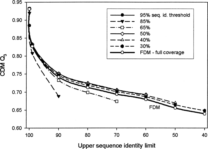
▶ illustrates the dependence of accuracy on the upper sequence identity limit as a function of the sequence identity threshold and shows that the sequence identity threshold of 50% gives the highest prediction accuracy Q3 of CDM. It also displays the strong dependence of the performance of CDM on the upper sequence identity limit. The sharp drop in the accuracy of prediction when almost identical sequences are removed clearly demonstrates the importance of the availability of highly homologous sequences for successful secondary structure prediction. This strong dependence explains why secondary structure predictions fail to reach high accuracies, signifying the limitation of short-range treatments in prediction algorithms.
Figure 3.
Accuracy of prediction Q3 of the Consensus Data Mining method as a function of the upper sequence identity limit. The different curves were obtained by varying the sequence identity thresholds. The sequence identity threshold of 50% gives the best results. At 50% threshold, CDM always performs better than individual FDM applied to the whole sequence (full coverage).
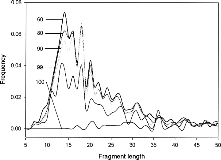
We have also analyzed the length of the fragments predicted by FDM in the final consensus predictions (▶). The results are shown as a function of the limit to upper sequence identities. When the upper sequence identity limit is 100%, the fragment lengths are distributed almost evenly, showing only two small peaks around 21 and 36. The rest of the plots show similar curves peaking around 14, 16, 18, and 20. With decreasing upper sequence identity limit, more FDM predicted fragments are utilized in CDM: The numbers of fragments are 510, 716, 974, 1046, 1097, and 1153 for the upper sequence identity limits of 100, 99, 90, 80, 70, and 60, respectively. Lower values of the upper sequence identity limit, however, decrease the average length of fragments.
Figure 4.
The length distribution of fragments predicted by FDM in CDM as a function of upper sequence identity limit. The sequence identity threshold is 50%. The upper sequence identity limit values are identified for the individual curves
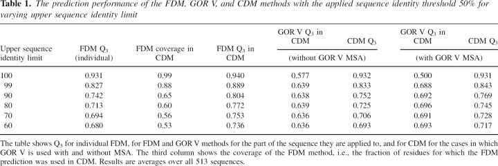
▶ shows the prediction accuracies of the individual FDM; FDM and GOR V methods for the sequence regions they are applied to; and the consensus (CDM) method, for a range of upper sequence identities. The coverage of the FDM method is also shown (coverage of a specific method is defined as the fraction of residues predicted by this method used in the consensus prediction). The average cross-validated (by the jack-knife methodology) accuracy of individual GOR V prediction is 73.5% when MSA and heuristic rules (see below) are used. In the absence of MSA, the jack-knifed accuracy drops to 67.5%. Note that the accuracy of individual GOR IV predictions (previous version) was 64.4%. The 2.9% difference arises as a result of the heuristic rules based on the length of helix and β-sheet predictions: If their lengths are too short (e.g., helices shorter than five residues or sheets shorter than three residues), these predictions are converted to coil.
Table 1.
The prediction performance of the FDM, GOR V, and CDM methods with the applied sequence identity threshold 50% for varying upper sequence identity limit
The table shows Q3 for individual FDM, for FDM and GOR V methods for the part of the sequence they are applied to, and for CDM for the cases in which GOR V is used with and without MSA. The third column shows the coverage of the FDM method, i.e., the fraction of residues for which the FDM prediction was used in CDM. Results are averages over all 513 sequences.
The identification of ranges of parameters where CDM gives better performance than individual methods is crucial. The data in ▶ clearly demonstrate that, when the upper sequence identity limit is ≥90%, CDM confers a higher accuracy than individual GOR V, with or without MSA. Additionally, on average CDM is always better for the entire sequence than individual FDM regardless of the upper sequence identity limit.
For the cases of 100% and 99% sequence identities, only a small portion of sequences are predicted by GOR V (1% and 12%, respectively). At these upper sequence identity limits, GOR V without MSA performs better than GOR V with MSA for this small number of cases. Only when the upper sequence identity limit falls to ≤90% does GOR V with MSA then perform better. Although it is generally assumed that adding multiple sequence alignments to predictions increases the accuracy, the data in ▶ clearly demonstrate that MSA is not effective for low sequence identities, rather the inclusion of MSA increases noise in the data.
Another interesting feature shown in ▶ is the coverage by the FDM method, i.e., the fraction of FDM predictions in the consensus CDM method. When the upper sequence identity limit drops from 100% to 90%, the FDM coverage plummets from 99% to 65%, illustrating the lack of aligned sequences with high identity. Compare this value with the 12% coverage lost when the upper sequence identity limit drops further from 90% to 60%.
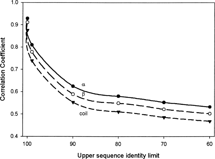
Another measure of prediction accuracy besides Q3 is the Matthews correlation coefficient. The correlation coefficients for three secondary structure elements, α-helices (H), β-sheets (E), and coil (C), are shown in ▶. The eight-letter DSSP alphabet has been reduced to the three-letter code as described in the Materials and Methods section. The plots in ▶ were obtained at the sequence identity threshold of 50% for a varying upper sequence identity. Similar to the majority of secondary structure algorithms, the correlation coefficients are highest for α-helices (H), followed by those for β-sheets (E), and lastly for coils (C). The correlation coefficients obtained by CDM show a consistent and smoother monotonic decrease with a decrease in the upper sequence identity limit.
Figure 5.
The Matthews correlation coefficients for CDM predictions for individual secondary structure elements as a function of the upper sequence identity limit. The eight-letter DSSP alphabet is reduced to three secondary structure elements as explained in the Materials and Methods section: α-helices (H), β-sheets (E), and coil (C). The results are obtained for the 50% sequence identity threshold. GOR V is used without MSA.
Replacing GOR V with PSIPRED in the Consensus Data Mining
To compare the performance of our Consensus Data Mining method based on GOR V with other popular secondary structure prediction algorithms, we have chosen the PSIPRED algorithm (Jones 1999) for detailed studies. First, we have computed the accuracy of prediction by PSIPRED on the Cuff and Barton (1999, 2000) data set of 513 sequences (CB513) used with the GOR V and CDM methods. The accuracy of prediction of the secondary structure with PSIPRED for the Cuff and Barton data set reaches Q3 ∼80%, i.e., it significantly exceeds the original accuracy of prediction of GOR V (73.5%). We should note, however, that the result of 80% is an overprediction of PSIPRED because the result is non-cross-validated. The PSIPRED database that is used for the Neural Network training contains some sequences similar to sequences in the CB513 data set. The most accurate comparison between GOR V and PSIPRED should be made by applying the CB513 database (used in GOR V) for the training of PSIPRED and full jack-knife for the prediction for the CB513 data set. Such an approach would likely decrease the accuracy of prediction of PSIPRED to ∼76%, i.e., to the currently cross-validated accuracy of prediction of the PSIPRED method. The advantage of the original CDM method with GOR V is that we have developed the codes of both GOR V and Fragments Data Mining programs that comprise the CDM algorithm, and we are able to run and fully control the CDM performance. Because of this, the computations using the original CDM method based on GOR V are much faster than similar computations using the CDM variant with PSIPRED, and it is easier for us to implement cross-validation.
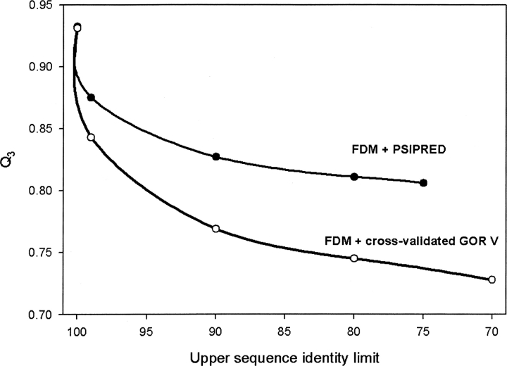
We have also developed a variant of the Consensus Data Mining method that uses PSIPRED instead of GOR V for the prediction when fragments with sufficiently high identities cannot be found in the database. These results are shown in ▶. We repeated the calculations for a set of sequence identity cutoff values ranging from 30% to 95%. We obtained the best performance with a 70% sequence identity cutoff for combining FDM with PSIPRED. The performance of the CDM method with PSIPRED exceeds the original CDM method based on GOR V, but, as we have discussed previously, we were not able to cross-validate these results.
Figure 6.
The comparison of prediction accuracy when cross-validated GOR V is replaced by PSIPRED in Consensus Data Mining. Note that the results obtained by PSIPRED are not cross-validated, and, with a proper cross-validation, the results may be expected to be ∼4%–5% less accurate.
Discussion
The accuracy of the secondary structure prediction is important for modeling the three-dimensional structures of proteins. In this work, we combined two previous successful methods, Fragment Database Mining (FDM) and GOR V, to develop the highly accurate Consensus Data Mining (CDM) method, based on the availability of aligned sequences of high similarity. The CDM method is an alternative to other currently available secondary structure prediction algorithms, especially when the multiple sequence alignments of high similarities are included in the predictions. Our results show that, on average, the accuracy of the method ranges from 67.5% to 93.2% depending on the sequence similarity of the target sequence to sequences in the PDB. This represents a significant improvement over the original GOR V method (accuracy with multiple sequence alignment, 73.5%) and, when a similar structure fragment is present, about a 1% gain––a slight, yet consistent, increase over the FDM method. Our hybrid method is adoptable to include additional structural information as the PDB grows. The results here show that it is preferable to include the structural information directly as structural fragments when they are available, and consequently this approach will ultimately supersede the entirely statistically based methods, such as GOR. Our consensus method shows that hybrid methods have the potential of improving secondary structure prediction performance of individual methods consistently. The improvement of secondary structure prediction accuracy will enhance tertiary structure prediction methods that employ secondary structure prediction as an input. Among those, homology modeling algorithms, such as MODELLER or SWISS-MODEL, have a potential for accuracy enhancement by incorporating CDM into their algorithms. For this purpose, we will implement a CDM server and make stand-alone software available in the near future.
Materials and methods
Database
The database of Cuff and Barton (1999, 2000) of 513 sequentially nonredundant domains has 84,107 residues and is used to test the new CDM method. (For details of the data set, see Cuff and Barton 1999, 2000.)
DSSP alphabet reduction
The Database of Secondary Structure in Proteins (DSSP) developed in 1983 by Kabsch and Sander (1983) is a widely used method for the assignment of the secondary structure based mostly on identification of hydrogen bonds in the crystallographic data. (There are, however, other alternative assignment methods, such as STRIDE [Frishman and Argos 1997] or, most recently, KAKSI [Martin et al. 2005]). DSPP classifies secondary structure elements into eight classes: H (α-helix), E (extended β-strand), G (310 helix), I (π-helix), B (bridge, a single residue β-strand), T (β-turn), S (bend), and C (coil). We follow a standard method of reduction of this eight-letter alphabet to the regular three-letter secondary structure code in the following manner: Helix (H) in the three-letter code includes three DSSP states, H, G, and I; β-strand (E) contains E and B; and coil (C) consists of T, S, and C.
GOR V (Kloczkowski et al. 2002; Sen et al. 2005)
The GOR method, proposed originally by Garnier, Osguthorpe, and Robson in 1978 (Garnier et al. 1978), is one of the first, important methods for prediction of secondary structure from sequence. The GOR method involves information theory and Bayesian statistics (Garnier et al. 1978; Gibrat et al. 1987; Garnier and Robson 1989; Garnier et al. 1996; Kloczkowski et al. 2002). The information entropy I can be written as a function of secondary structure S for a given amino acid R:
However, this function depends only on single-residue statistics. The predictions can be greatly improved by incorporating the information of flanking residues when a sliding window is used. For GOR V, a variable size window proved to produce the best results. Then, using relative informational content gives:
 |
In this equation, Ri represents the ith residue in the sliding window, S is a secondary structure of the jth residue (Sj), and n − S are all the conformations different than S. In the case when secondary structures are abstracted into three classes, S can be helix, sheet, or coil. n − S represents the other two secondary structures. Total information content can be expressed as
 |
If we keep information on single and pairs of residues, algebraic manipulation finally leads to
 |
for the residue site in the middle of the sliding window. In this equation, d is the number of flanking residues, and 2d + 1 is the size of the sliding window.
Over decades, the GOR method has been constantly improved by including larger databases and more detailed statistics, where these changes were gradually integrated into the first four versions of GOR. With these improvements, the Q3 accuracy reached 64% in GOR IV. However, studies by other groups showed that the accuracy of prediction for secondary structure prediction methods could be significantly increased by including evolutionary information through multiple sequence alignments (MSAs) (Zvelebil et al. 1987; Levin and Garnier 1988; Rost 1996; for a recent review, see Simossis and Heringa 2004). In the most recent GOR V (Kloczkowski et al. 2002), evolutionary information in the form of MSAs is included using PSI-BLAST (Altschul et al. 1997) (GOR V Server is available at http://gor.bb.iastate.edu; Sen et al. 2005). MSA is generated using PSI-BLAST with the nr database, allowing up to five iterations. MSA increases the information content and therefore allows an improved discrimination of secondary structures. In the last stage, heuristic rules related to the predicted secondary structure distribution are used to improve predictions. With the help of evolutionary information, the full jack-knifed prediction accuracy of GOR V using the Cuff and Barton data set attains Q3 = 73.5%, an almost 10% increase from the previous GOR IV performance. The segment overlap (SOV) (Zemla et al. 1999), an alternative to the Q3 measure of prediction accuracy, is also high at 70.8%. These results substantiate the reliability of GOR V algorithm in our consensus method: Although the algorithm does not provide as much accuracy as the prediction methods based on neural networks (i.e., PHD [Rost 1996]; PSIPRED [Jones 1999]), it can definitely be used as a complement to Fragment Database Mining, which performs poorly with fragments of low sequence similarity. In this work, we use GOR V without MSA (with Q3 accuracy 67.5%) and with MSA (accuracy of 73.5%) to test the performance of hybrid methods.
Fragment Database Mining (FDM)
FDM (Cheng et al. 2005) searches for sequences in the PDB similar to the target sequences and aligns the sequence hits for the secondary structure prediction. For a given target sequence the BLAST similarity alignment search is performed first. Matching segments from BLAST alignments are assigned weights according to their sequence similarity to fragments of the target sequence, followed by normalization. Several different parameters are taken into account in the weight assignment: various substitution matrices, a range of similarity/identity thresholds, degree of solvent exposure, and protein classification and sizes. The secondary structure for each residue in the target sequence is predicted based on the highest normalized score.
Local sequence alignments are obtained with BLAST on the Cuff and Barton (1999, 2000) data set CB513 using BLOSUM-45 (the best performance) and several other substitution matrices. We weighted fragments with a scoring based on their identity scores id and their powers idx, where x is a positive number. The value x = 3 was found to provide the optimum performance. For each position in the sequence, the secondary structure is predicted based on the secondary structures of the matching fragments at that position.
Consensus Data Mining (CDM)
CDM is a three-step algorithm based on the simple idea of combining two complementary secondary structure prediction methods, each with distinct strengths. In the first step, FDM calculations are performed for a given target sequence, and for each residue in the sequence, the normalized similarity score is computed. For some sites, the sequence identity could be as high as 100%. In the second step, the GOR V algorithm is applied to obtain a second set of secondary structure predictions. In the last step, a sequence identity threshold is defined to decide whether the FDM or the GOR V result will be used in the consensus prediction for a given residue. In the CDM method, the FDM predictions are used for the residues with an identity score above the sequence identity threshold, and the GOR V predictions are used for the residues with an identity score below the sequence identity threshold.
Prediction performance metrics
We used Q3 for the secondary structure prediction accuracy. In the accuracy matrix [Aij] of the size 3 × 3, i and j correspond to the three states H, E, C. The ijth element, Aij, of the accuracy matrix is defined as the number of residues predicted to be in state j, which are actually in state i. The diagonal entries of [Aij] are numbers of correctly predicted residues for each state, and Q3 is defined as:
 |
Here N is the number of residues in the query sequence. Matthews correlation coefficient is another measure of prediction accuracy defined for each secondary structure element separately. For example, the Matthews correlation coefficient for the helix (H) is:
 |
where TP, TN, FN, and FP with subscripts α are the numbers of true positives, true negatives, false negatives, and false positives for helices, respectively.
Acknowledgments
The authors acknowledge the financial support provided by the NIH grant 1R01GM072014 and R33GM066387.
Footnotes
Reprint requests to: Taner Z. Sen, L.H. Baker Center for Bioinformatics and Biological Statistics, Iowa State University, Ames, IA 50011-3020, USA; e-mail: taner@iastate.edu; fax: (515) 294-3841.
Article published online ahead of print. Article and publication date are at http://www.proteinscience.org/cgi/doi/10.1110/ps.062125306.
References
- Altschul, S.F., Madden, T.L., Schaffer, A.A., Zhang, J.H., Zhang, Z., Miller, W., and Lipman, D.J. 1997. Gapped BLAST and PSI-BLAST: A new generation of protein database search programs. Nucleic Acids Res. 25 3389–3402. [DOI] [PMC free article] [PubMed] [Google Scholar]
- Berman, H.M., Westbrook, J., Feng, Z., Gilliland, G., Bhat, T.N., Weissig, H., Shindyalov, I.N., and Bourne, P.E. 2000. The Protein Data Bank. Nucleic Acids Res. 28 235–242. [DOI] [PMC free article] [PubMed] [Google Scholar]
- Camacho, C.J. and Vajda, S. 2002. Protein–protein association kinetics and protein docking. Curr. Opin. Struct. Biol. 12 36–40. [DOI] [PubMed] [Google Scholar]
- Chaudhuri, A. and Chant, J. 2005. Protein-interaction mapping in search of effective drug targets. Bioessays 27 958–969. [DOI] [PubMed] [Google Scholar]
- Cheng, H., Sen, T.Z., Kloczkowski, A., Margaritis, D., and Jernigan, R.L. 2005. Prediction of protein secondary structure by mining structural fragment database. Polymer 46 4314–4321. [DOI] [PMC free article] [PubMed] [Google Scholar]
- Cuff, J.A. and Barton, G.J. 1999. Evaluation and improvement of multiple sequence methods for protein secondary structure prediction. Proteins 34 508–519. [DOI] [PubMed] [Google Scholar]
- Cuff, J.A. and Barton, G.J. 2000. Application of multiple sequence alignment profiles to improve protein secondary structure prediction. Proteins 40 502–511. [DOI] [PubMed] [Google Scholar]
- Frishman, D. and Argos, P. 1997. Seventy-five percent accuracy in protein secondary structure prediction. Proteins 27 329–335. [DOI] [PubMed] [Google Scholar]
- Garnier, J. and Robson, B. 1989. The GOR method for predicting secondary structures in proteins. In Prediction of protein structure and the principles of protein conformation (ed. G.D. Fasman), pp. 417–465. Plenum Press, New York.
- Garnier, J., Osguthorpe, D.J., and Robson, B. 1978. Analysis of the accuracy and implications of simple methods for predicting the decondary structure of globular proteins. J. Mol. Biol. 120 97–120. [DOI] [PubMed] [Google Scholar]
- Garnier, J., Gilbrat, J.F., and Robson, B. 1996. GOR method for predicting protein secondary structure from amino acid sequence. Methods Enzymol. 266 540–553. [DOI] [PubMed] [Google Scholar]
- Gibrat, J.F., Garnier, J., and Robson, B. 1987. Further developments of protein secondary structure prediction using information theory: New parameters and consideration of residue pairs. J. Mol. Biol. 198 425–443. [DOI] [PubMed] [Google Scholar]
- Halperin, I., Ma, B., Wolfson, H., and Nussinov, R. 2002. Principles of docking: An overview of search algorithms and a guide to scoring functions. Proteins 47 409–443. [DOI] [PubMed] [Google Scholar]
- Hua, S. and Sun, Z. 2001. A novel method of protein secondary structure prediction with high segment overlap measure: Support vector machine approach. J. Mol. Biol. 308 397–407. [DOI] [PubMed] [Google Scholar]
- Huang, X., Huang, D.S., Zhang, G.Z., Zhu, Y.P., and Li, Y.X. 2005. Prediction of protein secondary structure using improved two-level neural network architecture. Protein Pept. Lett. 12 805–811. [DOI] [PubMed] [Google Scholar]
- Jones, T.D. 1999. Protein secondary structure prediction based on position specific matrices. J. Mol. Biol. 292 195–202. [DOI] [PubMed] [Google Scholar]
- Kabsch, W. and Sander, C. 1983. A dictionary of secondary structure. Biopolymers 22 2577–2637. [DOI] [PubMed] [Google Scholar]
- Keskin, O., Ma, B., Rogale, K., Gunasekaran, K., and Nussinov, R. 2005. Protein–protein interactions: Organization, cooperativity and mapping in a bottom-up Systems Biology approach. Phys. Biol. 2 S24–S35. [DOI] [PubMed] [Google Scholar]
- Kihara, D. 2005. The effect of long-range interactions on the secondary structure formation of proteins. Protein Sci. 14 1955–1963. [DOI] [PMC free article] [PubMed] [Google Scholar]
- Kloczkowski, A., Ting, K.L., Jernigan, R.L., and Garnier, J. 2002. Combining the GOR V algorithm with evolutionary information for protein secondary structure prediction from amino acid sequence. Proteins 49 154–166. [DOI] [PubMed] [Google Scholar]
- Kolinski, A. 2004. Protein modeling and structure prediction with a reduced representation. Acta Biochim. Pol. 51 349–371. [PubMed] [Google Scholar]
- Kolinski, A. and Bujnicki, J.M. 2005. Generalized protein structure prediction based on combination of fold-recognition with de novo folding and evaluation of models. Proteins 61 84–90. [DOI] [PubMed] [Google Scholar]
- Levin, J.M. and Garnier, J. 1988. Improvements in a secondary structure prediction method based on a search for local sequence homologies and its use as a model building tool. Biochim. Biophys. Acta 955 283–295. [DOI] [PubMed] [Google Scholar]
- Lin, K., Simossis, V.A., Taylor, W.R., and Heringa, J. 2005. A simple and fast secondary structure prediction method using hidden neural networks. Bioinformatics 21 152–159. [DOI] [PubMed] [Google Scholar]
- Martin, J., Letellier, G., Marin, A., Taly, J.F., de Brevern, A., and Gibrat, J.F. 2005. Protein secondary structure assignment revisited: A detailed analysis of different assignment methods. BMC Struct. Biol. 5 17. [DOI] [PMC free article] [PubMed] [Google Scholar]
- Mendes, J., Guerois, R., and Serrano, L. 2002. Energy estimation in protein design. Curr. Opin. Struct. Biol. 12 441–446. [DOI] [PubMed] [Google Scholar]
- Nguyen, M.N. and Rajapakse, J.C. 2005. Two-stage multi-class support vector machines to protein secondary structure prediction. Pac. Symp. Biocomput. 10 346–357. [DOI] [PubMed] [Google Scholar]
- Park, S., Yang, X., and Saven, J.G. 2004. Advances in computational protein design. Curr. Opin. Struct. Biol. 14 487–494. [DOI] [PubMed] [Google Scholar]
- Rost, B. 1996. PHD: Predicting one-dimensional protein structure by profile-based neural networks. Methods Enzymol. 266 525–539. [DOI] [PubMed] [Google Scholar]
- Rost, B. 2001. Review: Protein secondary structure prediction continues to rise. J. Struct. Biol. 134 204–218. [DOI] [PubMed] [Google Scholar]
- Sen, T.Z., Kloczkowski, A., Jernigan, R.L., Yan, C., Honavar, V., Ho, K.M., Wang, C.Z., Ihm, Y., Cao, H., and Gu, X., et al. 2004. Predicting binding sites of hydrolase-inhibitor complexes by combining several methods. BMC Bioinformatics 5 205. [DOI] [PMC free article] [PubMed] [Google Scholar]
- Sen, T.Z., Jernigan, R.L., Garnier, J., and Kloczkowski, A. 2005. GOR V server for protein secondary structure prediction. Bioinformatics 21 2787–2788. [DOI] [PMC free article] [PubMed] [Google Scholar]
- Simossis, V.A. and Heringa, J. 2004. Integrating protein secondary structure prediction and multiple sequence alignment. Curr. Protein Pept. Sci. 5 249–266. [DOI] [PubMed] [Google Scholar]
- Smith, G.R. and Sternberg, M.J.E. 2002. Prediction of protein–protein interactions by docking methods. Curr. Opin. Struct. Biol. 12 28–35. [DOI] [PubMed] [Google Scholar]
- Solis, A.D. and Rackovsky, S. 2004. On the use of secondary structure in protein structure prediction: A bioinformatic analysis. Polymer 45 525–546. [Google Scholar]
- Szilagyi, A., Grimm, V., Arakaki, A.K., and Skolnick, J. 2005. Prediction of physical protein–protein interactions. Phys. Biol. 2 S1–S16. [DOI] [PubMed] [Google Scholar]
- Tovchigrechko, A., Wells, C.A., and Vakser, I.A. 2002. Docking of protein models. Protein Sci. 11 1888–1896. [DOI] [PMC free article] [PubMed] [Google Scholar]
- Tsai, C.J. and Nussinov, R. 2005. The implications of higher (or lower) success in secondary structure prediction of chain fragments. Protein Sci. 14 1943–1944. [DOI] [PMC free article] [PubMed] [Google Scholar]
- Vizcarra, C.L. and Mayo, S.L. 2005. Electrostatics in computational protein design. Curr. Opin. Chem. Biol. 9 622–626. [DOI] [PubMed] [Google Scholar]
- Wood, M.J. and Hirst, J.D. 2005. Protein secondary structure prediction with dihedral angles. Proteins 59 476–481. [DOI] [PubMed] [Google Scholar]
- Zemla, A., Venclovas, C., Moult, J., and Fidelis, K. 1999. Processing and analysis of CASP3 protein structure predictions. Proteins (Suppl. 3): 37 22–29. [DOI] [PubMed] [Google Scholar]
- Zvelebil, M.J., Barton, G.J., Taylor, W.R., and Sternberg, M.J.E. 1987. Prediction of protein secondary structure and active-sites using the alignment of homologous sequences. J. Mol. Biol. 195 957–961. [DOI] [PubMed] [Google Scholar]


