Identification of correct regions in protein models using structural, alignment, and consensus information

Abstract

In this study we present two methods to predict the local quality of a protein model: ProQres and ProQprof. ProQres is based on structural features that can be calculated from a model, while ProQprof uses alignment information and can only be used if the model is created from an alignment. In addition, we also propose a simple approach based on local consensus, Pcons-local. We show that all these methods perform better than state-of-the-art methodologies and that, when applicable, the consensus approach is by far the best approach to predict local structure quality. It was also found that ProQprof performed better than other methods for models based on distant relationships, while ProQres performed best for models based on closer relationship, i.e., a model has to be reasonably good to make a structural evaluation useful. Finally, we show that a combination of ProQprof and ProQres (ProQlocal) performed better than any other nonconsensus method for both high- and low-quality models. Additional information and Web servers are available at: http://www.sbc.su.se/~bjorn/ProQ/.

Automatic protein structure prediction has improved significantly over the last few years (Fischer et al. 1999, 2001, 2003). Most manual predictors participating in CASP (Moult et al. 2003) now actually perform worse than the best automatic prediction methods. However, there are still a few manual predictors that perform significantly better than the automatic methods (Kryshtafovych et al. 2005). Obviously, if we could completely understand what methods the manual predictors use, we should be able to construct computer programs that use the same schemes. One such scheme already implemented in the best automatic methods is the consensus analysis, where a multitude of different models produced by different methods are analyzed for structural consensus (Lundström et al. 2001; Fischer 2003; Ginalski et al. 2003; Wallner and Elofsson 2005b).

Another important step in structure prediction, commonly used by manual predictors, is to actually analyze the protein structure models in terms of correctness. Over the last decade, many different methods to analyze and evaluate protein structures have been developed. Most have focused on finding the native structure or native-like structures in a large set of decoys (Sippl 1990; Park and Levitt 1996; Park et al. 1997; Lazaridis and Karplus 1999; Gatchell et al. 2000; Petrey and Honig 2000; Vendruscolo et al. 2000; Vorobjev and Hermans 2001; Dominy and Brooks 2002; Felts et al. 2002; Wallner and Elofsson 2003). In these methods the overall quality of each protein structure model is assessed, and one single quality measure is obtained for the whole model. This is useful when the objective is to select the best possible model from a number of plausible models.

However, an alternative approach would be to use a method that assigns a local quality measure to each residue and thereafter combines the best parts from different models into a hybrid model using multiple templates. This technique could, in theory, produce models better than the best model in the set. In addition, the knowledge of which parts of a model that are correct and incorrect can be used as a guide during the refinement process and also provide confidence measures to different parts of protein models.

Methods that assign a local quality measure to each residue can use at least two different types of information, which we utilize in this study: structural or alignment information. The structural information can be calculated for any protein model, while the alignment information only can be obtained for models created from an alignment to known structure. The advantage of using two approaches is that they contain different types of information, e.g., two completely conserved residues will get a similar quality estimate based on the alignment, while a structural evaluation might reveal that one of them is better.

Currently, three, easily available, methods use structural information to predict the quality for each residue: Errat (Colovos and Yeates 1993), ProsaII (Sippl 1993), and Verify3D (Lüthy et al. 1992; Eisenberg et al. 1997). The two latter has been used successfully in CASP to select well- and poorly-folded fragments (Kosinski et al. 2003; von Grotthuss et al. 2003). All three are knowledge-based, i.e., they use statistical information from real proteins. Errat analyzes the statistics of nonbonded interactions between nitrogen (N), carbon (C), and oxygen (O) atoms. ProsaII utilizes the probability to find two residues separated at a specific distance. Verify3D derives a“3D-1D” profile based on the local environment of each residue, described by the statistical preferences for the following criteria: the area of the residue that is buried, the fraction of side-chain area that is covered by polar atoms (oxygen and nitrogen), and the local secondary structure.

Recently, we developed ProQ (Wallner and Elofsson 2003), a method that identifies correct and incorrect protein models by predicting the overall correctness of a model based on structural features. It was shown that ProQ was better at finding correct models than the overall correctness prediction made by Errat, ProsaII, and Verify3D. Possibly due to the use of several complementary structural features, but also because ProQ was trained to identify “correct” models rather than the exact native structure. “Correct” defined in a similar way as in Live-Bench (Rychlewski et al. 2003), CAFASP (Fischer et al. 2003), and CASP (Moult et al. 2003), i.e., by finding similar fragments between the native and a model.

One of the goals of this study was to develop a method, ProQres, that could identify correct and incorrect regions in protein models based on structural features. In essence, this problem is similar to the prediction of the overall correctness as done in ProQ, and therefore many of the steps in the development of ProQres were based on ideas from ProQ. For instance, we use a neural network based approach, as it should be able to find more subtle correlations than a purely statistical method. We also use similar structural features and a related target function. The main difference between ProQres and ProQ is that both the structural features and the target function are localized, i.e., the structural features describe a local environment of the protein structure and that the target function measures the local correctness instead of overall correctness.

As an alternative to structural information it is often possible to use alignment information to assess the quality of a model. This can be done by comparing the sequence similarity to assess the quality of the target-template alignment; this can be extended by using evolutionary information (profiles) for the target and/or the template sequence. Intuitively, aligned positions with similar profiles should be more likely to be correct. This was confirmed in a recent study where it was shown that regions in the models with a high-profile alignment score were more likely to be correct compared to regions with lower scores (Tress et al. 2003). In that study only the profile for the template sequence was used to calculate the alignment score. The predictor presented in this study, ProQprof, improves the method suggested by Tress et al. (2003) by utilizing profiles for both the model and the template sequence and a neural network to calculate the alignment score. Below we first introduce the target function, i.e., the measure of correctness, and thereafter the development of the two local quality predictors ProQres and ProQprof.

Target function

To be able to choose a suitable target function that identifies “correct” and “incorrect” residues in a protein model, a definition of the correctness is needed. The basic requirement is that a residue should be “correct” if its coordinates are close to what is observed in the native structure and “incorrect” if the coordinates deviate from the native structure. The average root mean square deviation (RMSD) after an optimal superposition between the model and the native structure is frequently used as a measure of protein structure similarity. A possible target function could be the RMSD for each residue between the model and the native structure. This measure will be low for “correct” and high for “incorrect” residues. However, instead of using this local RMSD measure directly, we used a measure similar to what used in the LGscore (Levitt and Gerstein 1998; Cristobal et al. 2001), MaxSub (Siew et al. 2000), and in TM-score (Zhang and Skolnick 2004). In these methods the RMSD values are scaled between 0 and 1 using the function:

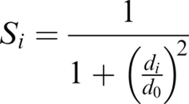where d_i is the distance (RMSD) between residue i in the native structure and in the model and d₀ is a distance threshold. This score, S_i, ranges from 1 for a perfect prediction to 0 when d_i goes to infinity. The distance threshold, d₀, defines the distance when S_i = 0.5, i.e., it monitors how fast the function should go to zero, we used 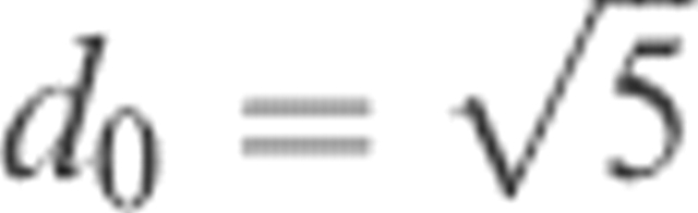as in LGscore and MaxSub. S_i was calculated from a superposition based on the most significant set of structural fragments as in LGscore (Cristobal et al. 2001), i.e., the superposition is only done on the better parts of the model (see Materials and Methods for a more detailed description). To our knowledge, S_i (hereafter called the S-score) has never been used to classify correctness on the residue level before. Still, we believe that this score is a useful measure of local structure correctness as it concentrates on the correct regions, both by scaling down all high RMSD values and by focusing the superposition on the most significant set of structural fragments. In addition the average S-score does not depend on the size of the model. From a machine-learning perspective it is also an advantage to use a function with numerically limited values. It can be seen in Figure 1 that this score is also able to find residues that were build on correct and incorrect alignments. Almost all residues with S-score above 0.6 are based on correct alignments, and 80% of all residues with S-score below 0.1 are based on incorrect alignments.

Figure 1.

The distribution of S-score and residue displacement. All residues were grouped by S-score and residue displacement relative to the STRUCTAL structural alignment. Residues off are the number of residues the alignment is shifted (displaced) compared to structural alignment (data taken from the hmtest set).

Development of ProQres

The structural features used in ProQres were identical to the ones in our earlier method ProQ (Wallner and Elofsson 2003), i.e., atom-atom contacts, residue-residue contacts, solvent accessibility surfaces, and secondary structure information. However, in order to achieve a localized quality prediction, the environment around each residue was described by calculating the structural features for a sliding window around the central residue. Hereby, the quality of the central residue is predicted not only by its own features, but also by contacts, solvent accessibility and secondary structure involving the residue in the window and their contacts.

Atom-atom contacts were represented as in Errat (Colovos and Yeates 1993); for each contact type the input to the neural networks was its fraction of all contacts. Contacts between the same 13 different atom types as used in ProQ were used, a reduced representation with only three atom types showed a much lower performance (data not shown). Residue-residue contacts were represented in a similar way with 20 amino acids grouped into six groups. Solvent accessibility surfaces were described by classifying each residue into one of four exposure bins and calculate the fraction of the six amino acid types in each bin. Secondary structure information was represented by the predicted probability from PSIPRED (Jones 1999b) for the observed secondary structure (see Materials and Methods for a more detailed description).

It is important to realize that there are clear nonlinearities in the data, and a high fraction of a certain atom-atom contact must be seen in the context of all the other fractions, e.g., it might be good to have one fraction high only if another is at a certain level, etc. This is probably one of the reasons why neural networks yield significantly higher correlations compared to a simple multiple linear regression using the same data (data not shown).

Neural networks were trained and optimized using different types of input data and the results are summarized in Table 1. The window size was optimized by training neural networks using window sizes ranging from 1 to 23. A nine-residue window seemed to be optimal for most types of input parameters and was therefore used below (Fig. 2).

Table 1.

The performance of neural networks trained with different types of input parameters

R, the highest correlation coefficient between the correct and predicted values; Z_1–3, the Z-score for separating residues with 1 Å RMSDs from residues with 3 A RMSDs, i.e., [(score 1 Å) – (score 3 Å)]/std(score).

For each combination of methods, the window size was optimized independently.

Figure 2.

Finding the optimal sequence window size for ProQres. Performance for neural nets trained using different window size to calculate the structural parameters.

It can be seen in Table 1 that atom-atom contacts and the solvent accessibility surfaces contain more information than residue-residue contacts. This is probably because there are much fewer residue-residue contacts compared to atom-atom contacts making the statistics less reliable. For the solvent accessibility surfaces low counts are not a problem, since the surface information is more independent compared to the residue-residue contacts and certain features are described more clearly, e.g., it is almost always unfavorable to expose hydrophobic residues, while a particular residue-residue contact might be either good or bad depending on the other contacts. In comparison with ProQ a smaller improvement was found by combining more than two different types of information, indicating that the overlap between the different structural features is greater for ProQres. However, although the improvement is small it is still significant with P < 0.001 using “Fisher's z' transformation” (Weisstein 2005). Therefore, it was decided to use all the structural features in the final predictor.

Development of ProQprof

Another method to predict the local quality of a protein model is to analyze the target-template alignment. Tress et al. (2003) used a profile-derived alignment score to predict reliable regions in alignments. They concluded that regions in the models with a high-profile alignment score were more likely to be correct compared to regions with lower scores. However, they only used a profile for one of the sequences. Here we derive a neural network-based predictor, ProQprof, that predicts local structure correctness based on profiles both for the target (model) and template sequence. The prediction is based on profile-profile scores, which reflects the similarity of two profile vectors. In addition to the profile-profile scores, the two last columns in the PSI-BLAST profile corresponding to information per position and relative weight of gapless real matches to pseudocounts were also used as input to the neural network. This extra information clearly improved the performance (Fig. 3). The improvement for including either the information content or the gap information was similar and including both only provided a marginal additional performance gain.

Figure 3.

Finding the optimal alignment window size for ProQprof. Performance for neural nets trained using different sizes for the profile score window. “Profile only” refers to using only a window of profile similarity scores as input; “IC” and “gap” refer to the two last columns in the PSI-BLAST profile, respectively.

The largest performance increase is obtained by the use of a window of profile-profile scores. Neural networks using a window consistently performed better than networks not using a window. The improvement is apparent already for a small three-residue window and the optimal performance is reached around 15 residues (Fig. 3; Table 1). The obvious advantage with the window approach is that it makes it possible to detect a correct position with a low score in an otherwise high-scoring region, and to ignore an incorrect position with a high score in an otherwise low scoring region.

Combining ProQres and ProQprof (ProQlocal)

ProQres and ProQprof predict the local quality of a residue using different types of information. ProQres evaluates the structure, while ProQprof bases the prediction on the alignment. Obviously, these two approaches provide complementary information, e.g., the structure might be OK, while the sequence similarity is low or vice versa. This suggests that it might be possible to reach a higher performance by combining the two approaches. Therefore, different techniques to combine ProQres and ProQprof were explored, including neural networks and multiple linear regression for a window of ProQres and ProQprof scores (data not shown). However, it turned out that a simple sum of the ProQres and ProQprof scores performed similar to the more elaborate techniques. Thus, the combination of ProQres and ProQprof, ProQlocal, is a simple sum of the two scores. The simplicity of the sum indicates that the essential information in ProQlocal is that the ProQres and ProQprof predictions should agree, i.e., if both predict high quality to a region it is probably correct, and if both predict low quality to a region it is probably incorrect. A schematic overview of ProQres, ProQres, and ProQlocal is illustrated in Figure 4.

Figure 4.

Schematic overview of the ProQprof and ProQres prediction schemes. ProQprof uses the target-template alignment for its prediction. Profiles are constructed for the target and template sequence. Profile-profile scores are calculated for aligned positions in the target-template alignment. The final prediction is done for the central residue in a window of profile-profile scores. ProQres analyzes the structure built from the target-template alignment. The prediction is based on the local structural environment around each residue described by structural features such as atom-atom and residue-residue contacts and surface accessibility (see Materials and Methods for details). Finally ProQres and ProQprof predictions are combined in ProQlocal using a simple sum of the two scores.

Consensus analysis

In addition to the methods described above, a simple method based on consensus analysis, Pcons-local, was also implemented. This approach is basically identical to the confidence assignment step in 3D-SHOTGUN (Fischer 2003). The idea is simple: to estimate the quality of a residue in a protein model, the whole model is compared to all other models for that protein by superimposing all models and calculating the S-score for each residue. The average S-score for each residue then reflects how conserved the position of a particular residue is. It is quite likely that correct positions are well conserved between all models and that incorrect positions are less conserved. One drawback with this method is that it is only possible to perform if there exist several models for the same target sequence. Consequently, Pcons-local could only be applied to the LB2 test set, see below.

Results and Discussion

In order to not overestimate the performance, it is important to test new methods on a set completely different from the one used in training. In addition, the training set used here is somewhat artificial, since it is based on structural alignments. Therefore, two independent sets of protein models not used in the training process were compiled for this purpose. One set based on LiveBench-2 alignments (LB2) and one set (hmtest) used in a recent homology modeling benchmark (Wallner and Elofsson 2005a). The two benchmark sets also represent two different levels of model correctness, the LB2 set contains many regions of poor quality, whereas the hmtest models have a much higher quality, comparable to the quality of the models based on structural alignment used for training (Table 2). This wide range of different model qualities makes it possible to benchmark the performance for both easy and hard modeling targets.

Table 2.

Description of the different test set

No. of models, the total number of models for which all methods could calculate a score; No. of residues, the total number of residues in the set; <S-score>, the average S-score for the residues; <RMSD_s>, the average scaled RMSD; No. of correct alignments, the number of positions that are not displaced compared to the structural alignment, i.e., correct.

^aPer definition.

The performances of ProQres, ProQprof, and ProQlocal were compared to three simple methods using alignment information and to four methods using structural information: ProsaII, Verify3D, Errat, and Pcons-local (described above). However, since Pcons-local use a consensus analysis it needs a number of different models for each target and could only be applied on the LB2 set.

We focused the evaluation on two different but related properties: the ability to identify correct and incorrect regions. Both of these abilities are desirable properties for a predictor of local structure quality. In earlier studies the focus has mostly been on either finding the best parts of a model (Tress et al. 2003) or finding the incorrect parts of an X-ray structure (Lüthy et al. 1992).

The local correctness of the models in the two sets was assessed by comparing the alignments used in the construction of the models to STRUCTAL structural alignments (Subbiah et al. 1993) to identify correctly and incorrectly aligned residues. A reasonable assumption is that if parts of the alignment (for which a model is built on) are identical to the structural alignment, these parts of the structure are most likely correct, and parts where the alignments differ are most likely incorrect. In addition, average scaled RMSD values were also calculated by superimposing the good parts of the models and the native structures (see Materials and Methods). Neither the structural alignment nor the scaled RMSD measure were used directly in the development of ProQres and ProQprof, and might therefore be less biased than to use the S-score for evaluation.

The analysis was done using Receiver Operating Characteristic (ROC) plots to measure the ability to detect correctly and incorrectly aligned residues. To facilitate the analysis of the ROC plots, the data was divided in to three parts: (1) methods using alignment information (Fig. 5), (2) methods using structural information (Fig. 6), and (3) the best methods from the two previous parts (Fig. 7).

Figure 5.

Performance comparison using ROC plots for methods using alignment information, i.e., ProQprof (thick), Profile-Profile window (thin), Profile-Profile no window (thick dotted), and Sequence-Profile window (thin dotted). The ability to find incorrectly and correctly aligned regions in both the LB2 (A and B, respectively) and the hmtest (C and D, respectively) sets was assessed.

Figure 6.

Performance comparison using ROC plots for methods using structural information, i.e., ProQres (thin), ProsaII (thick), Verify3D (thick dotted), and Errat (thin dotted). The ability to find incorrectly and correctly aligned regions in both the LB2 (A and B, respectively) and the hmtest (C and D, respectively) sets was assessed.

Figure 7.

Performance comparison using ROC plots for the best methods using alignment and/or structural information, i.e., Pcons-local (thick dotted), ProQlocal (thin dotted), ProQprof (thick), and ProQres (thin). The ability to find incorrectly and correctly aligned regions in both the LB2 (A and B, respectively) and the hmtest (C and D, respectively) sets was assessed.

In addition to the ROC plots, the ability to detect correct residues and incorrect residues were assessed by analyzing the 10% highest and lowest scoring residues in terms of average scaled RMSD and fraction of incorrectly aligned residues (Tables 3, 4) (using cutoffs in the range 5%–20% yields similar results, data not shown). The values in Tables 3 and 4 agree well with the overall results from the ROC plots, and we propose that this simple measure can be used in future benchmarks.

Table 3.

Results on LB2 for the 10% lowest and 10% highest scores from the different methods

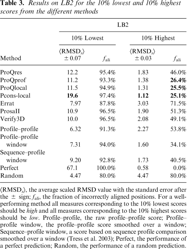
<RMSD_s>, the average scaled RMSD value with the standard error after the ± sign; f_ali, the fraction of incorrectly aligned positions. For a well- performing method all measures corresponding to the 10% lowest scores should be high and all measures corresponding to the 10% highest scores should be low. Profile–profile, the raw profile–profile score; Profile–profile window, the profile–profile score smoothed over a window; Sequence–profile window, a score based on sequence profile comparison smoothed over a window (Tress et al. 2003); Perfect, the performance of a perfect prediction; Random, the performance of a random prediction.

Table 4.

Results on hmtest for the 10% lowest and 10% highest scores from the different methods

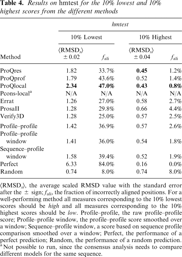
<RMSD_s>, the average scaled RMSD value with the standard error after the ± sign; f_ali, the fraction of incorrectly aligned positions. For a well-performing method all measures corresponding to the 10% lowest scores should be high and all measures corresponding to the 10% highest scores should be low. Profile–profile, the raw profile–profile score; Profile–profile window, the profile–profile score smoothed over a window; Sequence–profile window, a score based on sequence profile comparison smoothed over a window; Perfect, the performance of a perfect prediction; Random, the performance of a random prediction.

^aNot possible to run, since the consensus analysis needs to compare different models for the same sequence.

ProQprof, which uses a window of profile-profile scores to predict the quality of the residues in a model, was compared to three other methods using similar type of information: (1) raw profile-profile score, i.e., with no window; (2) profile-profile score triangularly smoothed over a window; and (3) our implementation of the sequence-profile score from Tress et al. (2003) also triangular smoothed over a window. From the ROC plot and the analysis of the highest and lowest scoring residues it is clear that ProQprof performs better than any of the simpler methods no matter which test set was used or if the ability to detect correct or incorrect residues was studied (Fig. 5; Tables 3, 4). Among the other methods, the triangular profile-profile score performs better than sequence-profile scores or the raw profile-profile score on LB2. However, on the hmtest set the sequence-profile is slightly better than the profile-profile score, indicating that profile-profile comparisons only have an advantage when the evolutionary distance between the two sequences is longer. This has also been shown in recent studies of profile-profile alignments (Ohlson et al. 2004; Wang and Dunbrack 2004).

Analogous to the comparison above, ProQres was compared to three methods also using structural information to assess the local quality: ProsaII, Verify3D, and Errat (Fig. 6). On the LB2 set, ProQres, ProsaII, and Verify3D perform very similarly, while Errat performs worse. But on hmtest, ProQres detects significantly more correctly and incorrectly aligned positions than the other methods (Fig. 6C,D). The average RMSD on the 10% highest (lowest) scoring residues from ProQres is 0.45 Å (1.82 Å) compared with 0.57 Å (1.28 Å) for the best of the other methods (Table 4). One possible explanation for the better performance of ProQres on the hmtest set is that the quality of the models in this set is more similar to the quality of the models in the training set (Table 2). However, neural networks trained on cross-validated data from LB2 did not perform significantly better on LB2 than the neural networks trained on the original training set (data not shown). Thus, the better performance of ProQres on the hmtest set is not a result of the set used for training. It is rather that a more detailed structural representation is needed to evaluate the high quality models in hmtest, while a reduced structural representation, as used in Pro-saII and Verify3D, is apparently sufficient to perform well on the LB2 set, but not for models of higher quality.

As a final test, the best alignment and structurally based methods from the previous two comparisons, ProQprof and ProQres, were compared to the combination, ProQlocal, and to the consensus method Pcons-local. Given the recent success of the consensus based approaches it is no surprise that Pcons-local is clearly better than the other methods (Fig. 7A,B). The performance difference seems to be slightly more pronounced for detecting incorrectly aligned residues (19.6 vs. 11.5 scaled RMSD and 97.4% vs. 95.4% incorrectly aligned residues among the lowest 10%) compared to detecting correctly aligned residues (1.12 vs. 1.31 scaled RMSD and 25.1% vs. 25.5% incorrectly aligned residues among the highest 10%) (Table 3). A possible explanation for this is that lack of consensus is usually a good indicator of incorrectness, while high consensus is not the only good indicator of correctness. The good performance of Pcons-local illustrates that the consensus approach is not only useful to select the best possible model, but is also a powerful tool that can be used to select the best and discard the worst parts of a model. It also emphasizes that whenever possible consensus should be used to assess protein structure models. Unfortunately, it is only possible to apply Pcons-local when a number of models for the target sequence exist. In addition, for the consensus analysis to be successful these models should be constructed using different techniques that exploit different aspects of the structure space available for a particular protein sequence. Fortunately, even though ProQprof is significantly worse than Pcons-local at detecting incorrectly aligned residues it is almost as good as Pcons-local at detecting correctly aligned residues. The performance of the highest scoring ProQprof residues in LB2 is actually quite impressive: only 25% incorrectly aligned residues compared to > 35% for all other structurally or alignment based methods (Table 3). The 10 percentage points performance gain of ProQprof over the Profile-profile window method is a result of the neural network training, as this score is essentially the input to the neural network.

In general, ProQprof performs slightly better than ProQres and much better on the identification of correct regions in the LB2 set. A comparison between Figure 7B and D indicates that the alignment information seem to be slightly more useful than structural information when the model quality is poor (on LB2), while structural information as used in ProQres gets more useful as the model quality gets higher (on hmtest). One reasonable explanation for this is that the local environment around the (few) correct residues in a poor model lacks many native interactions, making a structural evaluation useless. It makes sense that a model needs to be reasonably good to make a structural evaluation meaningful. A profile-profile comparison, on the other hand, is not dependent on conserved structural interactions; if the evolutionary history of two regions in an alignment are similar enough they will be given a high score irregardless of whether another part also score high.

Interestingly, ProQlocal performs better than ProQprof and ProQres alone, especially on the hmtest set (Fig. 7C,D). This shows that structural and alignment information can be combined to obtain a better predictor of local correctness. Since the combination is a simple sum of the ProQprof and ProQres score, the essential information used by the combined approach is that both the alignment and structurally based predictions should give similar answers; i.e., to predict a high combined score both methods must predict a high score, and to predict a low combined score both methods must predict a low score.

Conclusion

The aim of this study was to develop methods that predict the local correctness of a protein model. Two predictors were developed: ProQres, using structural information, and ProQprof, using alignment information. In addition, we also propose Pcons-local, a simple approach based on local consensus as used in Pcons and other fold recognition predictors. The final predictors were benchmarked against other methods for local structural evaluation as well as with standard methods for alignment analysis. We found that the novel methods performed better than state-of-the-art methodologies and that the consensus approach, Pcons-local, was the best method to predict local quality. It was also found that ProQprof performed better than other methods for models based on distant relationships, while ProQres performed best for models based on closer relationships.

Finally, we show that a combination of ProQprof and ProQres (ProQlocal) performed better than any other, nonconsensus, method for both high- and low-quality models. Additional information and Web servers are available at: http://www.sbc.su.se/~bjorn/ProQ/.

Materials and methods

Test and training data

All machine-learning methods start with the creation of a representative data set. The data set for this study was created by using STRUCTAL (Subbiah et al. 1993) to structurally align protein domains related on the family level according to SCOP (Murzin et al. 1995). Modeller6v2 (Sali and Blundell 1993) was then used to build protein models for each of the 840 alignments. In total, coordinates for 155,827 residues were constructed.

Additional test sets

As an additional independent test, the final methods were benchmarked on two different sets; LB2 derived from Live-Bench-2 (Bujnicki et al. 2001) and hmtest used in a recent homology modeling benchmark (Wallner and Elofsson 2005a).

LiveBench is continuously measuring the performance of different fold recognition Web servers by submitting the sequence of recently solved protein structures. To limit the number of models, only the first ranked model from the following servers were used: PDB-BLAST, FFAS (Rychlewski et al. 2000), Sam-T99 (Karplus et al. 1998), mGenTHREADER (Jones 1999a), INBGU, FUGUE (Shi et al. 2001), 3D-PSSM (Kelley et al. 2000), and Dali (Holm and Sander 1993).

The homology modeling benchmark set (hmtest) was constructed from alignments between protein domains related on the family level using pairwise global sequence alignment. The related domains have a sequence identity ranging from 30% to 100%. For both sets, Modeller6v2 (Sali and Blundell 1993) was used to generate the final models.

The properties of all benchmark sets are summarized in Table 2. LiveBench-2 has the lowest correctness, hmtest the highest, and the set used for training lies in between but closer to hmtest. The wide range of residue correctness makes it possible to test the ability to detect both correct and incorrect positions.

Neural network training

Neural network training was done using fivefold cross-validation, with the restriction that two models of the same super-family had to be in the same set, to ensure having no similar models in the training and testing data.

For the neural network implementations, Netlab, a neural network package for Matlab (Bishop 1995; Nabney and Bishop 1995), was used. A linear activation function was chosen, as it does not limit the range of output, which is necessary for the prediction of the S-score. The training was carried out using error back-propagation with a sum of squares error function and the scaled conjugate gradient algorithm.

The neural network training should be done with a minimum number of training cycles and hidden nodes in order to avoid overtraining. The optimal neural network architecture and training cycles was decided by monitoring the test set performance during training and choosing the network with the best performance on the test set (Brunak et al. 1991; Nielsen et al. 1997; Emanuelsson et al. 1999). We know that this is a problem since it involves the test set for optimizing the training length, and the performance might not reflect true generalization ability. However, practical experience has shown the performance on a new, independent test to be as correct as that found on the data set used to stop the training (Brunak et al. 1991; Wallner and Elofsson 2003). Also, the final comparison to existing methods was done using data completely different from the training data. If two networks performed equally well, the network with the least number of hidden nodes was chosen. Since the training was performed using fivefold cross-validation, five different networks were trained each time. The output of the final predictor is the average of all five networks.

Input parameters

Two sets of neural network models were trained, one based on structural features and one based on alignment information. In the neural networks using structural features the local environment around each residue in the protein models was described by the following features: atom-atom and residue-residue contacts, solvent accessibility surfaces and secondary structure information calculated over a sequence window. The neural networks using alignment information based its predictions on Log_Aver profile-profile scores (von Öhsen and Zimmer 2001) calculated from aligned positions in the alignment used to build the model (see below).

Atom-atom contacts

Different atom types are distributed nonrandomly with respect to each other in proteins. Protein models with many errors will have a more randomized distribution of atomic contacts compared to protein models with fewer errors (Colovos and Yeates 1993). Protein models from Modeller contain 167 nonhydrogen atom types, i.e., to use contacts between all of these would give a total of 14,028 different types of contacts, which is far too many. To reduce the number of parameters, the 167 atom types were grouped into thirteen different groups as described in Wallner and Elofsson (2003).

Two atoms were defined to be in contact if the distance between their centers were within 5 Å. The 5 Å cutoff was chosen by trying different cutoffs in the 3 Å to 7 Å range. All atom-atom contacts involving any atom within the sequence window were counted, i.e., both atom-atom contacts made within the window and atom-atom contacts made from the window to atoms outside the window, ignoring contacts between atoms from positions adjacent in the sequence, since they would always be in contact. Finally, the number of atom-atom contacts from each group was divided by the total number of atom-atom contacts in the window. Thus, the atom-atom contact input vector consisted of the fraction of all the 91 different types of pairwise atom-atom contacts, e.g., fraction of carbon-carbon contacts and fraction of nitrogen-oxygen contacts, etc.

Residue-residue contacts

Different types of residues have different probabilities for being in contact with each other; for instance, hydrophobic residues are more likely to be in contact than two positively charged residues. To minimize the number of parameters, the 20 amino acids were grouped into six different residue types: (1) Arg, Lys (+); (2) Asp, Glu (−); (3) His, Phe, Trp, Tyr (aromatic); (4) Asn, Gln, Ser, Thr (polar); (5) Ala, Ile, Leu, Met, Val, Cys (hydrophobic); (6) Gly, Pro (structural).

Two residues were defined as being in contact if the distance between the Ca -atoms or any of the atoms belonging to the side chain of the two residues were within 5 Å and if the residues were more than five residues apart in the sequence (many different cutoffs in the range 3–12 Å were tested, and 5 Å showed the best performance). Identical to the data generation for the atom-atom contacts, all contacts involving any residue within the sequence window were counted, i.e., both residue-residue contacts made within (if more than five residues apart) and from the window to outside the window. Finally, the number of residue-residue contacts was divided by the total number of residue-residue contacts in the window. Thus, the residue-residue input vector consisted of the fraction of all the 21 different types of pairwise residue-residue contacts, e.g., fraction of hydrophobic-hydrophobic (group 5-group 5) and fraction of polar-hydrophobic (group 4-group 5), etc.

Solvent accessibility surfaces

The exposure of different residues to the solvent is also distributed nonrandomly in protein models. For instance, a part of a protein model with many exposed hydrophobic residues or buried charges is not likely to be of high quality.

Lee and Richards solvent accessibility surfaces were calculated using a probe with the size of a water molecule (1.4 Å radius) using the program Naccess (Lee and Richards 1971). The relative exposure of the side chains for each of the six residue groups was used, i.e., to which degree the side chain is exposed relative to the exposure of the particular amino acid in an extended ALA-x-ALA conformation. The exposure data was grouped into one of the four groups < 25%, 25%–50%, 50%–75%, and >75% exposed, and finally, normalized by dividing with the number of residues in the window. The solvent accessibility surface input vector consisted of 24 values, one for each residue type and exposure bin, e.g., (group 1, < 25%) corresponds to the fraction of residues from group 1 (Arg, Lys) that are < 25% exposed within the window, and so on for all six residue types and the four exposure bins.

Predicted secondary structure

If the predicted and the actual secondary structure in the protein model agree, there is a higher chance that that part of the structure is correct, and vice versa if they disagree. To put this into numbers, STRIDE (Frishman and Argos 1995) was used to assign secondary structure to the protein model based on its coordinates. Each residue was assigned to one of three classes: helix, sheet, or coil. This assignment was compared to the secondary structure prediction made by PSIPRED (Jones 1999b) for the same residues. For each residue the predicted probability from PSIPRED for the particular secondary structure class from STRIDE was taken as input to the neural network. Thus, the secondary structure input vector consisted only of one single value, the probability from PSIPRED for the secondary structure of the central residue within the window, e.g., if the central residue was in a helix the probability for helix was used, etc.

Alignment information

To derive input parameters to the neural networks using alignment information, profiles were obtained for both the model sequence and the template sequence after ten iterations of PSI-BLAST version 2.2.2 (Altschul et al. 1997). The search was performed against nrdb95 (Holm and Sander 1998) with a 10⁻³ E-value cutoff and all other parameters at default settings. Based on the alignment the corresponding profiles vectors were scored using the Log_Aver scoring function (described below), this scoring function was among the best in a recent fold-recognition benchmark (Ohlson et al. 2004). Other scoring functions such as PICASSO (Heger and Holm 2003) showed similar performance but overall the exact choice did not seem to be crucial.

The Log_Aver profile-profile score

Log_Aver (von Öhsen and Zimmer 2001) does not use the exact profiles from PSI-BLAST, but the distribution frequencies directly. The reason is that the substitution matrix is included in the comparison. The Log_Aver score is defined as:

where α and β are frequency vectors, and BLOSUM62_ij is the value in the BLOSUM62 substitution matrix for amino acid i replaced with j.

Triangular smoothing

To calculate a single score from a window of scores, triangular smoothing of the raw profile-profile scores was applied using the following formula:

where S_i is the profile-profile score for position i. This formula was also used in the implementation of the sequence-profile-derived score developed by Tress et al. (2003).

Target function

In this study, we have used S-score to give a measure of correctness to each residue in a protein model. This score was originally developed by Levitt and Gerstein (1998), and is now used in many of the functions to measure a protein model's quality, including MaxSub (Siew et al. 2000), LGscore (Cristobal et al. 2001), and TM-score (Zhang and Skolnick 2004). The S-score is defined as:

where d_i is the distance between residue i in the native and in the model, and d₀ is a distance threshold. The score, S_i, ranges from 1 for a perfect prediction (d_i = 0) to 0 when d_i goes to infinity; the distance threshold defines for which distance the score should be 0.5. In this way, it also monitors how fast the function should go to zero. The distance threshold was set to , and S_i was calculated from a superposition based on the most significant set of structural fragments in the same way as in LGscore. The significance of a set of structural fragments is estimated by calculating distributions of the sum of S_i dependent on the total fragment length for structural alignments of unrelated proteins. From this distribution, a significance value (P-value) for a set of structural fragments dependent on the sum of S_i and the length of the fragments can be calculated. A heuristic algorithm to find the most significant fragment is outlined in Cristobal et al. (2001).

Performance measures

Most of the performance comparisons were done using Receiver Operator Characteristics (ROC) plots, i.e., plotting the number of correct hits for an increasing number of incorrect hits. This was used to evaluate both the ability to detect correct aligned positions as well as incorrect aligned positions. In the analysis of the highest and lowest scoring positions, average scaled RMSD and fraction of incorrectly aligned positions were used.

The average scaled RMSD was calculated by superimposing the “good” parts of the model with the correct native structure, as described above. This superposition was then used to calculate the RMSD for each residue in the model. Finally, the quality of the residues were ranked using the different methods and average scaled RMSDs for the top 10% and lowest 10% for each method were calculated. The RMSD values were scaled using the following formula when calculating the average:

and then transformed back to RMSD using

The fraction of incorrectly aligned positions were calculated from the same set of residues as the average RMSD, i.e., the highest 10% and lowest 10% according to the score of the particular method. Residues in the alignment displaced relative to the structural alignment calculated using STRUCTAL (Subbiah et al. 1993) were considered incorrect.

References

- Altschul S.F., Madden T.L., Schaffer A.A., Zhang J., Zhang Z., Miller W., Lipman D.J. 1997. Gapped BLAST and PSI-BLAST: A new generation of protein database search programs Nucleic Acids Res. 25: 3389–3402. [DOI] [PMC free article] [PubMed] [Google Scholar]
- Bishop C.M. In Neural networks for pattern recognition. . 1995. Oxford University Press, Oxford,UK.
- Brunak S., Engelbrecht J., Knudsen S. 1991. Prediction of human mRNA donor and acceptor sites from the DNA sequence J. Mol. Biol. 220: 49–65. [DOI] [PubMed] [Google Scholar]
- Bujnicki J.M., Elofsson A., Fischer D., Rychlewski L. 2001. Live-bench-2: Large-scale automated evaluation of protein structure prediction servers Proteins 45: 184–191. [DOI] [PubMed] [Google Scholar]
- Colovos C. and Yeates T.O. 1993. Verification of protein structures: Patterns of nonbonded atomic interactions Protein Sci. 2: 1511–1519. [DOI] [PMC free article] [PubMed] [Google Scholar]
- Cristobal S., Zemla A., Fischer D., Rychlewski L., Elofsson A. 2001. A study of quality measures for protein threading models BMC Bioinformatics 2:–5. [DOI] [PMC free article] [PubMed]
- Dominy B.N. and Brooks C.L. 2002. Identifying native-like protein structures using physics-based potentials J. Comput. Chem. 23: 147–160. [DOI] [PubMed] [Google Scholar]
- Eisenberg D., Lüthy R., Bowie J.U. 1997. VERIFY3D: Assessment of protein models with three-dimensional profiles Methods Enzymol. 277: 396–404. [DOI] [PubMed] [Google Scholar]
- Emanuelsson O., Nielsen H., von Heijne G. 1999. ChloroP, a neural network-based method for predicting chloroplast transit peptides and their cleavage sites Protein Sci. 8: 978–984. [DOI] [PMC free article] [PubMed] [Google Scholar]
- Felts A.K., Gallicchio E., Wallqvist A., Levy R.M. 2002. Distinguishing native conformations of proteins from decoys with an effective free energy estimator based on the OPLS all-atom force field and the Surface Generalized Born solvent model Proteins 48: 404–422. [DOI] [PubMed] [Google Scholar]
- Fischer D. 2003. 3D-SHOTGUN: A novel, cooperative, fold-recognition meta-predictor Proteins 51: 434–441. [DOI] [PubMed] [Google Scholar]
- Fischer D., Barret C., Bryson K., Elofsson A., Godzik A., Jones D., Karplus K.J., Kelley L.A., MacCallum R.M., Pawowski K.et al. 1999. CAFASP-1: Critical assessment of fully automated protein structure prediction methods. Proteins Suppl 3: 209–217. [DOI] [PubMed] [Google Scholar]
- Fischer D., Elofsson A., Rychlewski L., Pazos F., Valencia A., Rost B., Ortiz A.R., Dunbrack R.L. 2001. CAFASP2: The second critical assessment of fully automated structure prediction methods Proteins Suppl 5: 171–183. [DOI] [PubMed] [Google Scholar]
- Fischer D., Rychlewski L., Dunbrack R.L., Ortiz A.R., Elofsson A. 2003. CAFASP3: The third critical assessment of fully automated structure prediction methods Proteins 53: 503–516. [DOI] [PubMed] [Google Scholar]
- Frishman D. and Argos P. 1995. Knowledge-based protein secondary structure assignment Proteins 23: 566–579. [DOI] [PubMed] [Google Scholar]
- Gatchell D.W., Dennis S., Vajda S. 2000. Discrimination of near-native protein structures from misfolded models by empirical free energy functions Proteins 41: 518–534. [PubMed] [Google Scholar]
- Ginalski K., Elofsson A., Fischer D., Rychlewski L. 2003. 3D-Jury: A simple approach to improve protein structure predictions Bioinformatics 19: 1015–1018. [DOI] [PubMed] [Google Scholar]
- Heger A. and Holm L. 2003. Exhaustive enumeration of protein domain families J. Mol. Biol. 328: 749–767. [DOI] [PubMed] [Google Scholar]
- Holm L. and Sander C. 1993. Protein structure comparison by alignment of distance matrices J. Mol. Biol. 233: 123–138. [DOI] [PubMed] [Google Scholar]
- 1998. Removing near-neighbour redundancy from large protein sequence collections Bioinformatics 14: 423–429 ——. [DOI] [PubMed] [Google Scholar]
- Jones D.T. 1999a. GenTHREADER: An efficient and reliable protein fold recognition method for genomic sequences J. Mol. Biol. 287: 797–815. [DOI] [PubMed] [Google Scholar]
- 1999b. Protein secondary structure prediction based on position-specific scoring matrices J. Mol. Biol. 292: 195–202 ——. [DOI] [PubMed] [Google Scholar]
- Karplus K., Barrett C., Hughey R. 1998. Hidden Markov models for detecting remote protein homologies Bioinformatics 14: 846–856. [DOI] [PubMed] [Google Scholar]
- Kelley L.A., MacCallum R.M., Sternberg M.J. 2000. Enhanced genome annotation using structural profiles in the program 3D-PSSM J. Mol. Biol. 299: 523–544. [DOI] [PubMed] [Google Scholar]
- Kosinski J., Cymerman I.A., Feder M., Kurowski M.A., Sasin J.M., Bujnicki J.M. 2003. A “FRankenstein's monster” approach to comparative modeling: Merging the finest fragments of fold-recognition models and iterative model refinement aided by 3D structure evaluation Proteins 53: 369–379. [DOI] [PubMed] [Google Scholar]
- Kryshtafovych A., Venclovas C., Fidelis K., Moult J. 2005. Progress over the first decade of CASP experiments Proteins 61: 225–236. [DOI] [PubMed] [Google Scholar]
- Lazaridis T. and Karplus M. 1999. Discrimination of the native from misfolded protein models with an energy function including implicit solvation J. Mol. Biol. 288: 477–487. [DOI] [PubMed] [Google Scholar]
- Lee B. and Richards F.M. 1971. The interpretation of protein structures: Estimation of static accessibility J. Mol. Biol. 55: 379–400. [DOI] [PubMed] [Google Scholar]
- Levitt M. and Gerstein M. 1998. A unified statistical framework for sequence comparison and structure comparison Proc. Natl. Acad. Sci. 95: 5913–5920. [DOI] [PMC free article] [PubMed] [Google Scholar]
- Lüthy R., Bowie J.U., Eisenberg D. 1992. Assessment of protein models with three-dimensional profiles Nature 356: 283–285. [DOI] [PubMed] [Google Scholar]
- Lundström J., Rychlewski L., Bujnicki J., Elofsson A. 2001. Pcons: A neural-network-based consensus predictor that improves fold recognition Protein Sci. 10: 2354–2362. [DOI] [PMC free article] [PubMed] [Google Scholar]
- Moult J., Fidelis K., Zemla A., Hubbard T. 2003. Critical assessment of methods of protein structure prediction (CASP)-round V Proteins 53: 334–339. [DOI] [PubMed] [Google Scholar]
- Murzin A.G., Brenner S.E., Hubbard T., Chothia C. 1995. SCOP: A structural classification of proteins database for the investigation of sequences and structures J. Mol. Biol. 247: 536–540. [DOI] [PubMed] [Google Scholar]
- Nabney I. and Bishop C. 1995. Netlab: Netlab neural network software. http://www.ncrg.aston.ac.uk/netlab/.
- Nielsen H., Engelbrecht J., Brunak S., von Heijne G. 1997. Identification of prokaryotic and eukaryotic signal peptides and prediction of their cleavage sites Protein Eng. 10: 1–6. [DOI] [PubMed] [Google Scholar]
- Ohlson T., Wallner B., Elofsson A. 2004. Profile-profile methods provide improved fold-recognition: A study of different profile-profile alignment methods Proteins 57: 188–197. [DOI] [PubMed] [Google Scholar]
- Park B. and Levitt M. 1996. Energy functions that discriminate X-ray and near native folds from well-constructed decoys J. Mol. Biol. 258: 367–392. [DOI] [PubMed] [Google Scholar]
- Park B.H., Huang E.S., Levitt M. 1997. Factors affecting the ability of energy functions to discriminate correct from incorrect folds J. Mol. Biol. 266: 831–846. [DOI] [PubMed] [Google Scholar]
- Petrey D. and Honig B. 2000. Free energy determinants of tertiary structure and the evaluation of protein models Protein Sci. 9: 2181–2191. [DOI] [PMC free article] [PubMed] [Google Scholar]
- Rychlewski L., Jaroszewski L., Li W., Godzik A. 2000. Comparison of sequence profiles. Strategies for structural predictions using sequence information Protein Sci. 9: 232–241. [DOI] [PMC free article] [PubMed] [Google Scholar]
- Rychlewski L., Fischer D., Elofsson A. 2003. Livebench-6: Large-scale automated evaluation of protein structure prediction servers Proteins 53: 542–547. [DOI] [PubMed] [Google Scholar]
- Sali A. and Blundell T.L. 1993. Comparative modelling by statisfaction of spatial restraints J. Mol. Biol. 234: 779–815. [DOI] [PubMed] [Google Scholar]
- Shi J., Blundell T.L., Mizuguchi K. 2001. Fugue: Sequence-structure homology recognition using environment-specific substitution tables and structure-dependent gap penalties J. Mol. Biol. 310: 243–257. [DOI] [PubMed] [Google Scholar]
- Siew N., Elofsson A., Rychlewski L., Fischer D. 2000. Maxsub: An automated measure to assess the quality of protein structure predictions Bioinformatics 16: 776–785. [DOI] [PubMed] [Google Scholar]
- Sippl M.J. 1990. Calculation of conformational ensembles from potentials of mean force. An approach to the knowledge-based prediction of local structures in globular proteins J. Mol. Biol. 213: 859–883. [DOI] [PubMed] [Google Scholar]
- 1993. Recognition of errors in three-dimensional structures of proteins Proteins 17: 355–362 ——. [DOI] [PubMed] [Google Scholar]
- Subbiah S., Laurents D.V., Levitt M. 1993. Structural similarity of DNA-binding domains of bacteriophage repressors and the globin core Curr. Biol. 3: 141–148. [DOI] [PubMed] [Google Scholar]
- Tress M.L., Jones D., Valencia A. 2003. Predicting reliable regions in protein alignments from sequence profiles J. Mol. Biol. 330: 705–718. [DOI] [PubMed] [Google Scholar]
- Vendruscolo M., Najmanovich R., Domany E. 2000. Can a pairwise contact potential stabilize native protein folds against decoys obtained by threading? Proteins 38: 134–148. [DOI] [PubMed] [Google Scholar]
- von Grotthuss M., Pas J., Wyrwicz L., Ginalski K., Rychlewski L. 2003. Application of 3D-Jury, GRDB, and Verify 3D in fold recognition Proteins 53: 418–423. [DOI] [PubMed] [Google Scholar]
- von Öhsen N. and Zimmer R. 2001. Improving profile-profile alignments via log average scoring In WABI'01: Proceedings of the first international workshop on algorithms in bioinformatics pp. 11–26. Springer-Verlag, London,UK.
- Vorobjev Y.N. and Hermans J. 2001. Free energies of protein decoys provide insight into determinants of protein stability Protein Sci. 10: 2498–2506. [DOI] [PMC free article] [PubMed] [Google Scholar]
- Wallner B. and Elofsson A. 2003. Can correct protein models be identified? Protein Sci. 12: 1073–1086. [DOI] [PMC free article] [PubMed] [Google Scholar]
- 2005a. All are not equal: A benchmark of different homology modeling programs Protein Sci. 14: 1315–1327 ——. [DOI] [PMC free article] [PubMed] [Google Scholar]
- 2005b. Pcons5: Combining consensus, structural evaluation and fold recognition scores Bioinformatics 21: 4248–4254 ——. [DOI] [PubMed] [Google Scholar]
- Wang G. and Dunbrack R.L. 2004. Scoring profile-to-profile sequence alignments Protein Sci. 13: 1612–1626. [DOI] [PMC free article] [PubMed] [Google Scholar]
- Weisstein E.W. 2005. Fisher's z'-transformation http://mathworld.wolfram.com/Fishersz-Transformation.html/.
- Zhang Y. and Skolnick J. 2004. Scoring function for automated assessment of protein structure template quality Proteins 57: 702–710. [DOI] [PubMed] [Google Scholar]