Revisiting the Voronoi description of protein–protein interfaces

Abstract

We developed a model of macromolecular interfaces based on the Voronoi diagram and the related alpha-complex, and we tested its properties on a set of 96 protein–protein complexes taken from the Protein Data Bank. The Voronoi model provides a natural definition of the interfaces, and it yields values of the number of interface atoms and of the interface area that have excellent correlation coefficients with those of the classical model based on solvent accessibility. Nevertheless, some atoms that do not lose solvent accessibility are part of the interface defined by the Voronoi model. The Voronoi model provides robust definitions of the curvature and of the connectivity of the interfaces, and leads to estimates of these features that generally agree with other approaches. Our implementation of the model allows an analysis of protein–water contacts that highlights the role of structural water molecules at protein–protein interfaces.

Proteins make noncovalent interactions that are essential elements of their biological function. The study of such interactions relies in part on modeling the geometry and physical chemistry of the interfaces built by interacting proteins. When atomic coordinates are available, the Voronoi description of proteins is a useful geometric tool that has been applied in a variety of settings. The pioneering work of Richards (1974) used the Euclidean Voronoi diagram to analyze the atomic packing inside macromolecules, followed by the work of many other investigators (Harpaz et al. 1994; Gerstein et al. 1995; Pontius et al. 1996; Nadassy et al. 2001; McConkey et al. 2002; Tsai and Gerstein 2002). The Voronoi diagram associates to each atom its Voronoi cell, a convex polyhedron that contains all points of space closer to that atom than to any other atom. More recently, it has been used to define contacts in macromolecules without applying a distance cutoff: Two atoms are in contact if and only if their Voronoi cells have a facet in common. Similarly, Voronoi cells can be drawn around amino acid residues to define residue–residue contacts (Singh et al. 1996; Munson and Singh 1997; Soyer et al. 2000; Dupuis et al. 2005). Given this definition of a contact, the set of facets shared by atoms of two macromolecules forming a complex represents their interface. There is, however, a major difficulty: Atoms on the molecular surface have unbounded, or at least poorly defined, Voronoi cells. This may be circumvented by surrounding the protein with solvent molecules (Soyer et al. 2000), but their position must be fixed, which is not physically meaningful. An alternative is to use the alpha-complex, an extension of the Voronoi diagram proposed by Edelsbrunner and Mucke (1994). Applications of the alpha-complex to macromolecules, reviewed by Poupon (2004), include the computation of molecular surfaces (Akkiraju and Edelsbrunner 1996), and that of interfaces in an implementation in which the unbounded facets that extend out of the molecular surface are removed by an iterative process called retraction (Ban et al. 2004). Cazals and Proust (2006) recently offered a simpler, and possibly more natural, way to define the interface between molecules by removing facets based on purely geometric criteria. Here, we apply their procedure to a set of 96 protein–protein complexes taken from the Protein Data Bank (PDB) (Berman et al. 2002), and compare the results to those of the classical approach where interfaces are defined by changes in solvent accessibility (Chothia and Janin 1975; Janin and Chothia 1990; Jones and Thornton 1995, 1996; Lo Conte et al. 1999; Chakrabarti and Janin 2002).

Methods and Results

A Voronoi model of macromolecular interfaces based on the alpha-complex

The Euclidean Voronoi diagram assumes that all atoms have the same radii, and its application to molecules must make approximations to fit atoms of different sizes (Richards 1974; Harpaz et al. 1994; Pontius et al. 1996). A closely related geometric construction provides a mathematically correct way to accommodate different radii: the “power diagram,” in which the Euclidean distance is replaced by the power distance with respect to a sphere (Gellatly and Finney 1982; Aurenhammer 1987). The power of a point x relative to a sphere of radius r centered at point a is:

Points x that have the same power relative to two spheres belong to the radical plane of the spheres, which contains their intersection if it exists. Given two atoms A₁ and A₂ represented by two balls (hard spheres) of radii r₁ and r₂ centered at a₁ and a₂, we may also define the power of A₁ relative to A₂, or A₂ relative to A₁:

When p(A₁, A₂) = 0, the two balls are orthogonal (they intersect at a right angle).

The power diagram reduces to the Voronoi diagram when all the balls have the same radius. Thus, we shall call it also a Voronoi diagram and associate it with its dual, the “Delaunay triangulation.” This is built by drawing edges spanning pairs of atoms that have a Voronoi facet in common, triangles spanning triplets that have a common Voronoi edge, and tetrahedra spanning quartets that have a common Voronoi vertex. In Figure 1A, the Delaunay triangulation includes four vertices placed at the centers of the four atoms, six edges linking these atoms, and three triangles. The Voronoi facets shared by the four atoms are drawn (in two dimensions) as lines orthogonal to the Delaunay edges; three of them extend outside the molecular surface and are unbounded.

Figure 1.

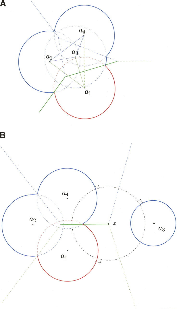
Delaunay and Voronoi descriptions of a protein–protein interface. Atoms are drawn as balls centered in a₁ for the red molecule, and a₂, a₃, and a₄ for the blue molecule. The ball radii are group radii augmented of the water probe radius. (A) Condition α: Delaunay edges are drawn in blue between the blue atoms and in green between blue and red atoms; the green edge between A₁ and A₄ is dashed to indicate that it is not part of the alpha-complex for α = 0. Thus, the interface between the red and the blue molecules comprises only the two Voronoi facets drawn in a thick green line. (B) Condition β: The dashed circle represents a ball orthogonal to the balls representing atoms A₁, A₃, and A₄. Its radius being m, the facet between A₁ and A₄ (thick green line) will be accepted or discarded depending on the ratio m/r, where r is the radius of A₁.

Noting that the power diagram is invariant if the same quantity α is added to all the square radii, Edelsbrunner and Mucke (1994) introduced the “alpha-complex.” For a given α, the alpha-complex is built as the Delaunay triangulation, except that one restricts each Voronoi cell to its associated ball and seeks intersections between these restricted regions. Thus, a Delaunay edge between two atoms is drawn if and only if the common facet lies inside the associated balls. This condition, which we shall call condition α, is satisfied in Figure 1A by the facets drawn in full line between atoms A₁ and A₂ or A₃. These facets are inside the balls representing the atoms, and the Delaunay edges spanning these atoms are part of the alpha-complex. In contrast, the facet between A₁ and A₄, drawn in dashes is entirely outside the balls, and the a₁a₄ edge is not part of the alpha-complex for this particular value of α. If we increase α, all the square radii increase and more facets satisfy condition α, until the alpha-complex reduces to the standard Delaunay triangulation at large values of α.

In our implementation, the ball radii are atomic or group radii augmented of the water probe radius, and α = 0. Under these conditions, the surface of the union of the balls, represented in two dimensions by arcs of circles drawn in full lines in Figure 1A, is the solvent-accessible surface as defined by Lee and Richards (1971). In a complex between two molecules, we color their atoms in red and in blue, respectively, and represent the interface by the set of bicolor Voronoi facets associated with the Delaunay edges linking atoms of different colors in the alpha-complex. In Figure 1A, the interface comprises the two facets orthogonal to the a₁a₂ and a₁a₃ edges, but not the facet between A₁ or A₄ due to condition α. These facets are drawn in green, whereas those in blue are internal to the blue molecule.

With large molecules such as proteins, condition α imposes a stringent selection that removes from the interface nearly all of the facets that stick out of the molecular surface. Nevertheless, some unbounded or excessively large facets remain, such as the one between A₁ and A₂ in Figure 1A. These are discarded based on “condition β”:

where r is the radius of the smaller of the two balls, and m is the radius of the largest ball orthogonal to the balls representing the two atoms. M is a threshold value that we set to M = 5 after checking that the number of discarded facets is very small (0.16%) and that similar results are obtained for M in the range 2.4–7. Condition β is illustrated by Figure 1B; there, r is the radius of A₁ and m is that of the ball drawn in dashes. This ball is centered at the Voronoi vertex x defined by A₁, A₃, and A₄, it is orthogonal to the three balls representing these atoms, and it is the largest ball orthogonal to A₁ and A₄. Condition α rejects the facet between A₁ and A₃, and condition β accepts or rejects the facet between A₁ and A₄, depending on the value of M.

Computing the Delaunay triangulation of a collection of balls and, subsequently the alpha-complex, is demanding in terms of efficiency and numerical issues. Our implementation is based upon the Alpha_shape_3 package of the CGAL library (http://www.cgal.org), and it is accessible at http://bombyx.inria.fr/Intervor/intervor.html.

The sample of protein–protein interfaces

The sample used in calculations here comprises protein–protein interfaces in 96 entries of the Protein Data Bank listed in Table 1. The calculation deals either with the proteins alone (AB model) or with the proteins and the structural water reported into the entry (ABW model). In the latter case, the sample is restricted to 30 entries reporting crystal structures at 2 Å resolution or better (2 Å set), as the water structure is likely to be less reliable in lower-resolution studies. We call AW–BW the protein–water interface of the ABW model. The sample is split in five classes: PI, complexes between proteases and protein inhibitors; ESI, complexes between enzymes other than proteases and protein substrates or inhibitors; AA, antigen–antibody complexes; ST, complexes involved in signal transduction or the cell cycle; and MI, miscellaneous complexes. All are nonobligate or transient assemblies in the sense of Nooren and Thornton (2003): A and B are proteins that fold separately and remain independent entities until they associate.

Table 1.

Protein–protein complexes

All protein atoms are tagged as A or B and included in the calculations. Water molecules, ignored in the AB model, appear in the ABW model if their crystallographic temperature factor is <80 Ų and are considered as part of the interface if they make at least one contact with atoms of both A and B. Other nonprotein atoms (HETATM in PDB entries) are included and tagged as U (unknown). Group radii are taken from Chothia (1976): C atoms, 1.87 Å aliphatic/1.76 Å trigonal; N atoms, 1.65 Å neutral/1.50 Å charged; O atoms, 1.4 Å; S atoms, 1.85 Å; and all other atoms, 2.0 Å. These radii are augmented of the probe radius (1.4 Å) for the Voronoi construction.

Size of the interfaces

In the AB model, interface atoms are all atoms of protein A (respectively, B) that share a Delaunay edge with an atom of protein B (respectively, A) in the alpha-complex for α = 0. The set of the bicolor facets dual of such edges constitutes the interface. Thus, the size of an interface can be evaluated in at least three ways: by counting interface atoms (N_Vor), counting facets (N_facet), or computing the Voronoi interface area VIA as the sum of the individual facet areas. In the classical approach, interfaces are sets of atoms that lose solvent accessibility when a complex forms. Then, the interface size is commonly evaluated as a buried surface area (BSA), which is the difference between the solvent-accessible surface area (ASA) of the protein atoms in isolated A and B and in the complex (Chothia and Janin 1975). The solvent accessibility model has no equivalent to N_facet, but the number of atoms that lose accessibility should correspond to N_Vor, and the buried surface area, to the VIA. The data of Lo Conte et al. (1999) will be used for comparison with ours.

Counting atoms

Table 2 shows that the AB interfaces in our sample comprise an average of 239 atoms, but the range of N_Vor is wide (117–581) and the standard deviation is large. AA interfaces, which are the most regular in size, have an average of 208 atoms with a small standard deviation. All but one of the 28 AA interfaces have N_Vor in the range 160–260. Antigen–antibody interfaces are described as “standard size” in Lo Conte et al. (1999). The range N_Vor = 160–260, which corresponds to that standard size, also comprises a great majority (22 out of 29) of the PI interfaces, and 70% of the 96 interfaces in the set. ST interfaces tend to be larger and more heterogeneous in size than the other classes.

Table 2.

Geometric properties of the interfaces

Figure 2A shows that N_Vor is linearly correlated to the number N_at of atoms that lose ASA. For the 72 complexes common to our sample and that of Lo Conte et al. (1999), the correlation is excellent (R² = 0.992), but N_Vor exceeds N_at by ∼13%. This excess is present in similar proportion in all complexes. Thus, some atoms that share facets with atoms of the other protein do not lose solvent accessibility. An examination of individual interfaces indicates that two-thirds of the atoms that contribute to N_Vor but not N_at have zero or nearly zero ASA in the isolated A or B components. Most belong to the protein main chain and are largely buried by their covalent environment. Figure 3 shows an example of that situation: The red ball is an atom of A that, when its neighbors in A are removed, is seen to intersect the blue ball figuring an atom of B; when the neighbors are present, the red ball is completely screened and has no solvent-accessible surface. There are also cases of solvent-accessible atoms that have bicolor facets yet do not lose ASA in the complex. In addition, 0.12% of the atoms that lose ASA are not counted in N_Vor because they contribute only to facets that do not pass condition β.

Figure 2.

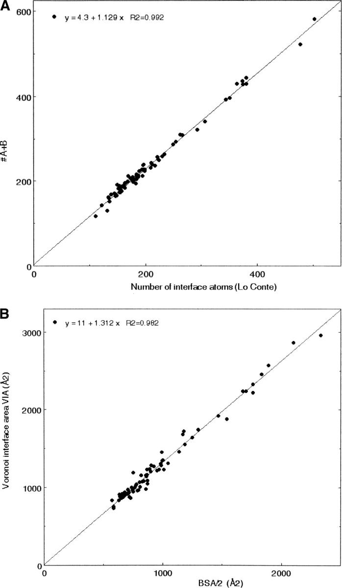
Comparison of the Voronoi and solvent accessibility models of protein–protein interfaces. Data for the solvent accessibility model are taken from Lo Conte et al. (1999). (A) Number of interface atoms in the Voronoi AB model (N_Vor) vs. atoms that lose ASA (N_at). The slope of the line is 1.13; the correlation coefficient, 0.992. (B) Voronoi interface area VIA vs. half of the buried surface area. The slope of the line is 1.31; the correlation coefficient, 0.982.

Figure 3.

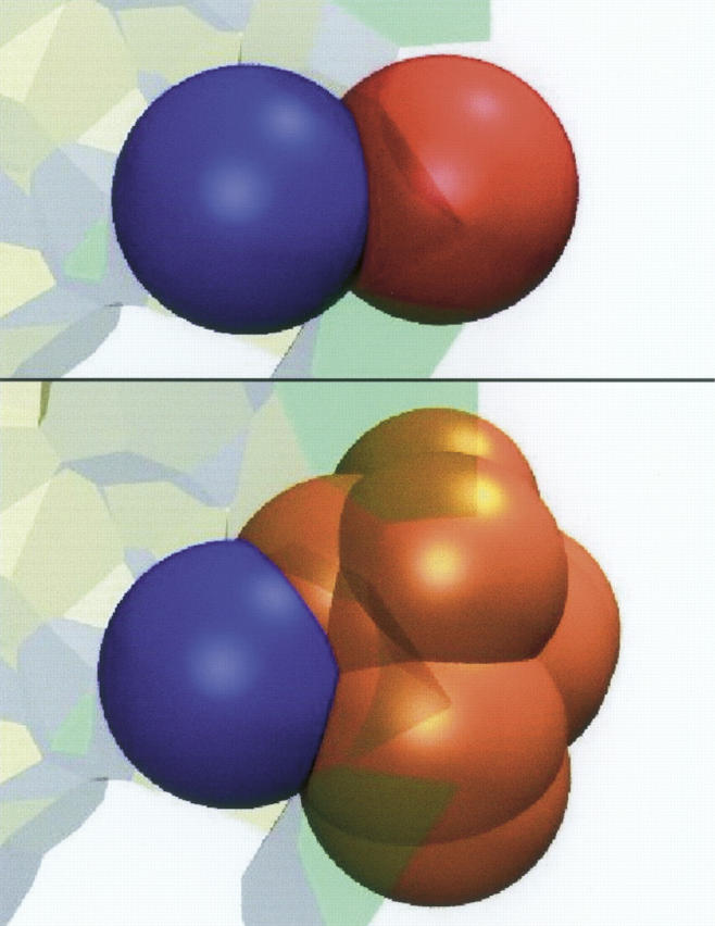
A solvent-inaccessible atom that is part of the Voronoi interface. Balls representing atoms have radii equal to the group radius plus the water probe radius (1.4 Å). The red ball is an atom of A; the blue ball, an atom of B. On top, the two balls are seen to intersect, and both atoms are part of the AB interface. On bottom, balls representing other atoms of A occlude the red ball; these atoms were omitted in the top part of the figure.

N_Vor increases in the ABW model due to atoms that share a facet with an interface water molecule but not with atoms of the other protein component. These atoms are part of the protein–water interface but not the AB interface. On average in the 30 entries of the 2 Å set, N_Vor is 45% larger in the ABW than the AB model, the ABW interface comprising 330 protein atoms and 34 water molecules.

To test whether A and B may make equal contributions N_A and N_B to N_Vor, we evaluated the ratio:

r_AB measures the asymmetry of the contributions. Its average value, 1.22 in our sample, is larger (1.47) in PI interfaces. As often noted, protease active sites tend to have a concave shape and the inhibitors a complementary convex shape, and the concave surface contributes more atoms to the interface than the convex one. In the extreme case of the kallikrein-pancreatic trypsin inhibitor complex (2kai), the protease contributes twice as many atoms as the inhibitor. In contrast, r_AB has a low value (1.11) in the AA class, compatible with the observation that antibodies raised against protein antigens tend to have flat combining sites (Mariuzza et al. 1987; MacCallum et al. 1996). Table 2 indicates that ST interfaces resemble AA interfaces from this point of view.

Counting facets

AB interfaces contain N_facet = 423 bicolor facets on average, that is, 1.77 facet per interface atom. As each facet implicates two atoms, the average interface atom has twice as many neighbors across the interface: n_neigh has an average of 3.53, a small standard deviation, and similar values in the five classes of complexes (Table 2). Thus, the linear correlation between the numbers of facets N_facet and of interface atoms N_Vor is excellent (R² = 0.984). In the ABW model, the average number of facets between protein atoms is essentially the same as in the AB model, but many new facets appear between protein atoms and water: Of the 769 facets reported in Table 2 for the average interface in the ABW model, 53% are with water molecules.

The facets vary widely in size. The facet area averages 3.0 Ų, but the median is only 1.65 Ų, and small facets with an area <1 Ų form 38% of the sample. Condition β removes excessively large facets, yet 5% of the facets retained have areas >10 Ų and up to 113 Ų.

Interface area

The Voronoi interface area (VIA) of the 96 interface ranges averages 1263 Ų with a broad range (733–2960 Ų) and a large standard deviation (Table 2). VIA is linearly related to N_Vor (R² = 0.964), to N_facet (R² = 0.926) in spite of the variability of the facet size, and also to BSA, the interface area defined by solvent accessibility. The correlation to the values of BSA reported by Lo Conte et al. (1999) is very good (R² = 0.982). Noting that two atoms that are in contact at an interface contribute twice to BSA but only once to VIA, the Voronoi model yields interface areas that are ∼31% larger than BSA/2 (Fig. 2B). In the ABW model, VIA increases by 30% as new protein atoms and water molecules become part of the interface.

Topology and shape

Connectivity

The Voronoi model provides a simple definition of “connected components” (cc) within an AB interface: A cc is a set of facets that have edges in common. On average, the 96 interfaces contain 1.90 cc. Some connected components were very small, and we removed those that contributed <7.5% of the VIA. Calling the remainder “significant connected components” (scc), we observe that the interfaces in our sample contain 1.21 scc on average. A large majority, 81 out of 96, have only one scc; nine have two, and six have three. All but two of the 29 PI interfaces and all but two of the 28 AA interfaces have a single scc. In contrast, multicomponent ST interfaces are common: seven out of 19.

We compared the scc to the patches of interface atoms defined by the geometric clustering procedure of Chakrabarti and Janin (2002) with a distance cutoff of 15 Å. Of 70 complexes analyzed by these investigators, 50 have an interface that has a single patch and also a single scc. In two cases, a single patch interface is split into two scc (Table 3), but the smaller of the two is only just above the 7.5% VIA cutoff. On the other hand, eight interfaces that form a single scc are split by the clustering algorithm. When both procedures split the interface, they do it in very similar ways: the fraction N_com/N_at of the atoms that belong both to the same patch and the same scc is at least 0.74. The very large interface of the Escherichia coli EF-Tu/Ts complex (1efu) is split into three scc and four patches (Fig. 4). The blue and green patches coincide with two of the scc, and the other two form a single large scc. In the ribonuclease–ribonuclease inhibitor complex (1dfj), the interface comprises three patches and three scc; one of the patches coincides with a scc, but the remainder of the interface is split in two different ways, so that the N_com/N_at fraction is only 0.74. In total, the two procedures yield identical results on 53 of the 70 interfaces; they disagree on the number of fragments in 11 cases including 1efu; in the remaining six interfaces, some of the patches do not coincide with an scc.

Table 3.

Patches versus connected components

Figure 4.

Interface connectivity: patches and scc. The Escherichia coli EF-Tu/Ts interface is split by the geometric clustering procedure of Chakrabarti and Janin (2002) into four patches, but it contains only three scc. (A) The patches are in different colors on the molecular surface of EF-Tu. (B) Heavy lines mark the edges of the three scc. EF-Ts is drawn as a red ribbon in both panels.

Water and connectivity

In the ABW model, connected components may be identified separately in the protein–protein interface AB and the protein–water interfaces AW–BW. In the 2 Å set, the average number of cc in an AB interface is 2.7; that of scc is 1.37, taking the same 7.5% VIA cutoff as above to define an scc (Table 2). Nine interfaces have two scc, and one interface has three. The AW–BW interface is much more fragmented and has an average of 6.6 cc. In a second step, we merge the connected components of the AB and the AW–BW interfaces that share a common edge. This reduces the number of cc, and the number of scc becomes one in all 30 interfaces of the 2 Å set. In other terms, interface water molecules connect the scc in all these interfaces.

Figure 5 illustrates the merging process in the chymotrypsin–eglin (1acb) and the transducin G_α–G_βγ (1got) complexes. The chymotrypsin–eglin interface is a standard-size PP interface. In the AB model, it forms a single scc with holes that contain water (Fig. 5A). In the ABW model, water in the larger hole splits the interface into two scc that the merging procedure fuses into one. In transducin, an ST archetype, the interface between G_α and G_βγ is larger than in 1acb and comprises two well-defined scc lined with water molecules (Fig. 5B). Some of these waters connect the scc and cause them to fuse during the merging procedure. In both examples, comparing the connectivities of the AB and ABW interfaces yields information on packing defects filled by water molecules.

Figure 5.

Water and the connectivity of protein–protein interfaces. (A) Chymotrypsin-eglin (1acb). The facets belong to the AB interface and form a single scc. In the ABW model, the interface is split into two scc marked by the heavy lines. Water is located around the interface and in the gap separating the two scc. (B) The transducin G_α–G_βγ interface (1got). The interface is in two parts, each lined by water molecules. They form a single scc in the AB model and two in the ABW model. In both 1acb and 1got, the two scc of the ABW model merge into one due to connecting waters.

Curvature

The curvature carried by a Voronoi edge ɛ may be defined as:

where β(ɛ) is the dihedral angle between the two bicolor facets sharing that edge, and l(ɛ) is the length of the edge (Cohen-Steiner and Morvan 2003). In Figure 6A, the two facets are shared by the Voronoi cell of an atom of A centered in a, and the cells of two atoms of B centered in b₁ and b₂. Alternatively, the facets may belong to an atom of B and two of A. By convention, β is positive in the first case and negative in the other. In the b₁ab₂ Delaunay triangle, the ab₁ and ab₂ edges represent noncovalent contacts atom A makes with B₁ and B₂. The b₁b₂ edge may be a covalent bond or a van der Waals contact. Its length is ∼1.5 Å in the first case and >3.5 Å in the other case. Thus, the absolute value of β, equal to the ∠b₁ab₂ angle, is likely to be smaller when B₁ and B₂ are covalently bonded. This is observed in the distribution of |β| (Fig. 6B), which is bimodal. The curvature is in the range of 12°–24° when B₁ and B₂ are covalently bonded and 20°–80° when the bond is noncovalent.

Figure 6.

Curvature. (A) An atom of protein A centered in a has common facets with two atoms of protein B centered in b₁ and b₂, and these facets share an edge, ɛ. The three atoms form a Delaunay triangle (heavy line). The discrete curvature at edge ɛ is the product of the length of the edge by the dihedral angle β, which is equal to the angle in a of the Delaunay triangle. (B) Distribution of the values of |β| in the 1udi interface. The peak near 15° represents triangles where the atoms centered in b₁ and b₂ are covalently linked. (C) The kallikrein–pancreatic trypsin inhibitor (2kai) interface, which has the largest mean curvature s_H = 17° in our sample, is concave toward the inhibitor drawn as a ribbon. The concavity is particularly marked around Lys 15 (drawn in van der Waals spheres), which occupies a well-defined pocket on the protease surface.

To get a global view of the shape of an interface, we may calculate a mean curvature angle by averaging h(ɛ) over all interior edges and normalizing by the total length of the edges:

The average value of s_H is 5.2°, but the range is wide: 0°–17°. The smaller values are for AA and ST interfaces. PI interfaces have larger mean curvatures, the largest value being for the kallikrein-pancreatic trypsin inhibitor complex (2kai) (Fig. 6C) as for the asymmetry ratio r_AB. In that interface, most pairs of facets are concave toward the inhibitor, and the local curvatures tend to add up. In a flat AA or ST interface, the two orientations are equally frequent, and local curvatures of opposite sign cancel. Thus, the shape information derived from the mean curvature is similar to that obtained above from the r_AB ratio.

Chemical composition, accessibility, and interactions

Chemical groups

The chemical composition of the facets that form the AB interfaces is given in Table 4: 58% of the facets involve a nonpolar (carbon-containing) chemical group; 30%, a neutral polar (O-, N-, S-containing) group; and 12%, a charged group from an Asp, a Glu, a Lys, or an Arg side chain. The nonpolar fraction is similar in the 96 interfaces, but charged groups are highly variable. The three types of chemical groups contribute, respectively, 56%, 29%, and 15% of the BSA in the sample analyzed by Lo Conte et al. (1999). Thus, the composition based on surface areas is similar to that obtained by counting Voronoi facets. Nevertheless, the composition of the set of atoms that contribute the facets is different: 65% nonpolar, 27% neutral polar, and 8% charged, which implies that the average polar or charged group contributes more facets than a nonpolar group. In addition, we noted above that ∼13% of the atoms that contribute to N_Vor do not lose ASA. This set of atoms is significantly enriched in nonpolar groups (73% vs. 65%) and lacks charged groups (2% vs. 8%), in line with the observation that a majority have zero ASA to start with, and the protein main chain contributes 58% of the set.

Table 4.

Chemical properties of the interfaces

Even though some interface atoms are already buried in free A or B, most remain accessible to solvent even in the complex. The fraction of the N_Vor interface atoms that have zero ASA in the complex is 35% on average, with a standard deviation of 7% and a wide range (13%–58%). This buried fraction is the same as in the solvent accessibility model (Lo Conte et al. 1999) in spite of the fact that there are 13% more interface atoms in the Voronoi model. When water is taken into account, many more interface atoms are buried, and the buried fraction increases sharply from 38% to 62% in the 2 Å set.

Interactions

A bicolor Voronoi facet indicates an interaction between an atom of A and one of B. The average number of interactions per interface atom is the same, n_neigh = 3.52, as the average number of neighbors. In Table 4, we distribute facets into three types that represent different types of interactions: nonpolar/nonpolar interactions between two carbon-containing groups; polar/polar interactions between two O-, N-, or S-containing groups; and nonpolar/polar interactions. On average, 44% of the facets are of the nonpolar/nonpolar type; 12%, polar/polar; and 44%, nonpolar/polar. In these statistics, charged groups count as polar, and only 1% of the facets represent a positive/negative charge interaction (salt bridge). These fractions are close to those expected for random pairing given the atomic composition of the interfaces. Statistics based on the contributions to the VIA rather than the number of facets give the same nonpolar/polar fraction (44%), a slightly lower nonpolar/nonpolar fraction (39%), and a larger (17%) polar/polar fraction that includes 2.9% of charge–charge interactions. The composition of the Voronoi facets reproduces the known atomic preferences for interfaces (Tsai et al. 1997; Lo Conte et al. 1999), but contact preferences at the atomic level are much less obvious (Robert and Janin 1998; Mintseris and Weng 2003), and their detection requires a more detailed statistical analysis.

In the ABW model, facets involving water molecules indicate the interaction of a protein atom with interface water, which we label water/polar or water/nonpolar, depending on the type of protein atom. Like Rodier et al. (2005), we find water-mediated interactions to be at least as abundant at interfaces as direct protein–protein interactions. The average number of bicolor facets in the 2 Å data set increases from 405 in AB to 769 in the ABW model. The additional interactions are 64% water/nonpolar and 36% water/polar, the same proportions as for nonpolar and polar protein atoms in N_Vor.

Discussion

The Voronoi construction has been extensively used to measure atomic volumes and describe the atomic packing inside proteins (Richards 1974; Harpaz et al. 1994; Gerstein et al. 1995; Pontius et al. 1996). Its first application to protein–protein interfaces was to show that they pack as densely as the protein interior by comparing the Voronoi volumes of interface atoms to those of atoms buried inside proteins (Janin and Chothia 1976; Lo Conte et al. 1999). Later applications include atomic and residue contacts (Munson and Singh 1997; McConkey et al. 2002). We use here an updated and enhanced implementation of that construction to define interfaces and examine their properties. Like Ban et al. (2004), we define a protein–protein interface by the set of facets shared by atoms of the two proteins after discarding excessively large facets that extend out of the protein surface. However, the way we treat the large facets is more direct, and it leads to significantly different results when applied to a set of protein–protein complexes taken from the PDB. In addition, our construction defines accessibility to solvent and handles water molecules, which were not considered by Ban et al. (2004).

Geometric and chemical features of protein–protein interfaces that have been examined in studies based on solvent accessibility are easily retrieved in our model. The Voronoi and solvent accessibility models are in good agreement concerning the size of the interfaces, expressed either as the number of atoms or a surface area. The observed correlation between the numbers N_Vor and N_at of interface atoms is very high, as well as the correlation between the areas VIA and BSA. Ban et al. (2004) cite values of a surface area similar to the VIA for 70 complexes analyzed by Chakrabarti and Janin (2002) and included in this study. They report a correlation with BSA values of 0.85, whereas we obtain 0.982. As both constructions apply the alpha-complex to atomic protein models, the better fit to the solvent accessibility model must be attributed to the different way in which we handle the large facets on the protein surface.

Although the solvent accessibility model and our implementation of the Voronoi model agree on the size of the interfaces, they differ in their definition of interface atoms. Both models find the same fraction of the interface atoms to be buried in the complex, and all atoms that lose solvent accessibility are part of the Voronoi interface. However, the converse is not true: A remarkable result of our study is the presence at interfaces of atoms that are already buried in the component subunits. In the complex, these atoms share Voronoi facets with one or several atoms of the other component, yet removing that component does not make them accessible to a water probe. They do not contribute to the hydrophobic effect and, being mostly nonpolar, may form few polar interactions. But they contribute to van der Waals interactions and to the close packing of the interface. A solvent-accessible atom may also fail to lose accessibility because the additional contacts it makes in the complex concern a region of its surface that is buried in the component subunit. We find that the solvent accessibility criterion misses ∼13% of the interface atoms for that reason. Main-chain atoms, which account for 19% of the BSA (Lo Conte et al. 1999), represent 39% of N_Vor and are a majority among the interface atoms that do not lose accessibility. Thus, the Voronoi model suggests that the protein main chain plays a role in protein–protein interaction that is even more important than suggested by previous studies.

The Voronoi model also gives a quantitative basis to features that are not easily estimated otherwise. For instance, the connectivity of an interface has a simple definition: Connected components are sets of bicolor facets that have edges in common. By that criterion, a majority of the interfaces in Table 1 are singly connected, a single scc including all or nearly all of the facets. The larger interfaces may contain two or three scc of comparable size. Interfaces have been split in various ways in the past, for instance, by considering segments of the protein sequence (Jones and Thornton 1997) or by clustering interface atoms based on a distance criterion (Chakrabarti and Janin 2002; Reichmann et al. 2005). The geometric clustering procedure of Chakrabarti and Janin (2002) distributes interface atoms into patches that are essentially identical to an scc in three-quarters of the complexes of Table 3, and in most other cases, it splits an scc into two patches as in Figure 4. Thus, the two approaches yield very similar results, but the Voronoi definition does not depend on a cutoff distance as does the clustering procedure.

The curvature of interface is another parameter that can be defined in the Voronoi model. The quantity h(ɛ) measured at a Voronoi edge (Equation 5) is an extension to a polyhedral surface, of the mean curvature of a smooth surface (Cohen-Steiner and Morvan 2003). Its sign indicates whether the interface is locally convex toward the A or the B component of the complex. When h(ɛ) is averaged over the whole interface to yield the s_H angle (Equation 6), the large value obtained for some PI complexes reflects the complementary concave/convex surfaces of the protease and the inhibitor. In AA and ST complexes, the interaction involves mostly flat patches on the protein surfaces, and s_H is small. The curvature defined by h(ɛ) is distinct from the angle deficiency of Ban et al. (2004), which is estimated at the vertexes of Voronoi polyhedra, not at their edges. It also differs from the planarity estimated by fitting a least-squares plane through the interface atoms (Argos 1988; Jones and Thornton 1996), yet the same qualitative conclusions can be drawn concerning the shapes of different classes of interfaces.

Unlike the solvent accessibility model, which identifies the interface atoms (albeit not all of them) but says nothing about their partners in the other subunit, the Voronoi model identifies the pairs in contact in a natural way without requiring a distance cutoff. This property has been used to analyze contacts and generate empirical potentials between protein atoms (Munson and Singh 1997; McConkey et al. 2002). We show here that the Voronoi model also handles protein–water interactions, which are abundant at protein–protein interfaces (Janin 1999; Rodier et al. 2005). Our data highlight the role of structural water, which fills packing defects and links together the components of interfaces that are split into several scc when only protein atoms are taken into account.

As a conclusion, we believe that this study introduces a new tool to analyze interactions between biological macromolecules and give a geometric, topological, and chemical description of their interfaces starting at the atomic level.

References

- Akkiraju N. and Edelsbrunner H. 1996. Triangulating the surface of a molecule. Discrete Appl. Math. 71: 5–22. [Google Scholar]
- Argos P. 1988. An investigation of protein subunit and domain interfaces. Protein Eng. 2: 101–113. [DOI] [PubMed] [Google Scholar]
- Aurenhammer F. 1987. Power diagrams: Properties, algorithms and applications. SIAM J. Computing 16: 78–96. [Google Scholar]
- Ban Y.E.A., Edelsbrunner H., Rudolph J. 2004. Interface surfaces for protein–protein complexes. Proceedings of the Eighth Annual International Conference on Research in Computational Molecular Biology (RECOMB 2004). San Diego, CA. pp. 205–212.
- Berman H.M., Battistuz T., Bhat T.N., Bluhm W.F., Bourne P.E., Burkhardt K., Feng Z., Gilliland G.L., Iype L., Jain S. et al. 2002. The Protein Data Bank. Acta Crystallogr. D Biol. Crystallogr. 58: 899–907. [DOI] [PubMed] [Google Scholar]
- Cazals F. and Proust F. 2006. Revisiting the Voronoi description of protein–protein interfaces: Algorithms. INRIA Research Rep. 5346. [DOI] [PMC free article] [PubMed]
- Chakrabarti P. and Janin J. 2002. Dissecting protein–protein recognition sites. Proteins 47: 334–343. [DOI] [PubMed] [Google Scholar]
- Chothia C. 1976. The nature of the accessible and buried surfaces in proteins. J. Mol. Biol. 105: 1–12. [DOI] [PubMed] [Google Scholar]
- Chothia C. and Janin J. 1975. Principles of protein–protein recognition. Nature 256: 705–708. [DOI] [PubMed] [Google Scholar]
- Cohen-Steiner D. and Morvan J.M. 2003. Restricted Delaunay triangulations and normal cycle. Proceedings of the Ninteenth Annual Symposium on Computational Geometry. New York, NY. pp. 312–321.
- Dupuis F., Sadoc J., Jullien R., Angelov B., Mornon J.P. 2005. Voro3D: 3D Voronoi tesselation applied to protein structures. Bioinformatics 21: 1715–1716. [DOI] [PubMed] [Google Scholar]
- Edelsbrunner H. and Mucke E.P. 1994. Three-dimensional α-shapes. ACM Trans. Graph. 13: 43–72. [Google Scholar]
- Gellatly B.J. and Finney J.L. 1982. Calculation of protein volumes: An alternative to the Voronoi procedure. J. Mol. Biol. 161: 305–322. [DOI] [PubMed] [Google Scholar]
- Gerstein M., Tsai J., Levitt M. 1995. The volume of atoms on the protein surface: Calculated from simulation, using Voronoi polyhedra. J. Mol. Biol. 249: 955–966. [DOI] [PubMed] [Google Scholar]
- Harpaz Y., Gerstein M., Chothia C. 1994. Volume changes on protein folding. Structure 2: 641–649. [DOI] [PubMed] [Google Scholar]
- Janin J. 1999. Wet and dry interfaces: The role of solvent in protein–protein and protein–DNA recognition. Struct. Fold. Des. 7: R277–R279. [DOI] [PubMed] [Google Scholar]
- Janin J. and Chothia C. 1976. Stability and specificity of protein–protein interactions: The case of the trypsin–trypsin inhibitor complexes. J. Mol. Biol. 100: 197–211. [DOI] [PubMed] [Google Scholar]
- Janin J. and Chothia C. 1990. The structure of protein–protein recognition sites. J. Biol. Chem. 265: 16027–16030. [PubMed] [Google Scholar]
- Jones S. and Thornton J.M. 1995. Protein–protein interactions: A review of protein dimer structures. Prog. Biophys. Mol. Biol. 63: 31–65. [DOI] [PubMed] [Google Scholar]
- Jones S. and Thornton J.M. 1996. Principles of protein–protein interactions. Proc. Natl. Acad. Sci. 93: 13–20. [DOI] [PMC free article] [PubMed] [Google Scholar]
- Jones S. and Thornton J.M. 1997. Analysis of protein–protein interaction sites using surface patches. J. Mol. Biol. 272: 121–132. [DOI] [PubMed] [Google Scholar]
- Lee B.K. and Richards F.M. 1971. The interpretation of protein structures: Estimation of static accessibility. J. Mol. Biol. 55: 379–400. [DOI] [PubMed] [Google Scholar]
- Lo Conte L., Chothia C., Janin J. 1999. The atomic structure of protein–protein recognition sites. J. Mol. Biol. 285: 2177–2198. [DOI] [PubMed] [Google Scholar]
- MacCallum R.M., Martin A.C., Thornton J.M. 1996. Antibody–antigen interactions: Contact analysis and binding site topography. J. Mol. Biol. 262: 732–745. [DOI] [PubMed] [Google Scholar]
- Mariuzza R.A., Phillips S.E., Poljak R.J. 1987. The structural basis of antigen–antibody recognition. Annu. Rev. Biophys. Biophys. Chem. 16: 139–159. [DOI] [PubMed] [Google Scholar]
- McConkey B.J., Sobolev V., Edelman M. 2002. Quantification of protein surfaces, volumes and atom–atom contacts using a constrained Voronoi procedure. Bioinformatics 18: 1365–1373. [DOI] [PubMed] [Google Scholar]
- Mintseris J. and Weng Z. 2003. Atomic contact vectors in protein–protein recognition. Proteins 52: 629–639. [DOI] [PubMed] [Google Scholar]
- Munson P. and Singh R. 1997. Statistical significance of hierarchical multi-body potentials based on the Delaunay tesselation and their application in sequence-structure alignment. Protein Sci. 6: 1467–1481. [DOI] [PMC free article] [PubMed] [Google Scholar]
- Nadassy K., Tomas-Oliveira I., Alberts I., Janin J., Wodak S.J. 2001. Standard atomic volumes in double-stranded DNA and packing of protein–DNA interfaces. Nucleic Acids Res. 29: 3362–3376. [DOI] [PMC free article] [PubMed] [Google Scholar]
- Nooren I.M. and Thornton J.M. 2003. Diversity of protein–protein interactions. EMBO J. 22: 3486–3492. [DOI] [PMC free article] [PubMed] [Google Scholar]
- Pontius J., Richelle J., Wodak S.J. 1996. Deviations from standard atomic volumes as a quality measure for protein crystal structures. J. Mol. Biol. 264: 121–136. [DOI] [PubMed] [Google Scholar]
- Poupon A. 2004. Voronoi and Voronoi-related tessellations in studies of protein structure and interaction. Curr. Opin. Struct. Biol. 14: 233–241. [DOI] [PubMed] [Google Scholar]
- Reichmann D., Rahat O., Albeck S., Meged R., Dym O., Schreiber G. 2005. The modular architecture of protein–protein binding interfaces. Proc. Natl. Acad. Sci. 102: 57–62. [DOI] [PMC free article] [PubMed] [Google Scholar]
- Richards F.M. 1974. The interpretation of protein structures: Total volume, group volume distributions and packing density. J. Mol. Biol. 82: 1–14. [DOI] [PubMed] [Google Scholar]
- Robert C.H. and Janin J. 1998. A soft, mean-field potential derived from crystal contacts for predicting protein–protein interaction. J. Mol. Biol. 283: 1037–1047. [DOI] [PubMed] [Google Scholar]
- Rodier F., Bahadur R.P., Chakrabarti P., Janin J. 2005. Hydration of protein–protein interfaces. Proteins 60: 36–45. [DOI] [PubMed] [Google Scholar]
- Singh R., Tropsha A., Vaisman I. 1996. Delaunay tesselation of proteins: Four body nearest-neighbour propensities of amino acid residues. J. Comput. Biol. 3: 213–221. [DOI] [PubMed] [Google Scholar]
- Soyer A., Chomilier J., Mornon J.P., Jullien R., Sadoc J. 2000. Voronoi tesselation reveals the condensed matter character of folded proteins. Phys. Rev. Lett. 85: 3532–3535. [DOI] [PubMed] [Google Scholar]
- Tsai J. and Gerstein M. 2002. Calculation of protein volumes: Sensitivity analysis and parameter database. Bioinformatics 18: 985–995. [DOI] [PubMed] [Google Scholar]
- Tsai C.J., Lin S.L., Wolfson H.J., Nussinov R. 1997. Studies of protein–protein interfaces: A statistical analysis of the hydrophobic effect. Protein Sci. 6: 53–64. [DOI] [PMC free article] [PubMed] [Google Scholar]