Normal-Mode Flexible Fitting of High-Resolution Structure of Biological Molecules toward One-Dimensional Low-Resolution Data

Abstract

We present a method for reconstructing a 3D structure from a pair distribution function by flexibly fitting known x-ray structures toward a conformation that agrees with the low-resolution data. This method uses a linear combination of low-frequency normal modes from elastic-network description of the molecule in an iterative manner to deform the structure optimally to conform to the target pair distribution function. A simple function, pair distance distribution function between atoms, is chosen as a test model to establish computational algorithms—optimization algorithm and scoring function—that can utilize low-resolution 1D data. To select a correct structural model based on less information, we developed a scoring function that takes into account a characteristic of pair distribution functions. In addition, we employ a new optimization algorithm, the trusted region method, that relies on both first and second derivatives of the scoring function. Illustrative results of our studies on simulated 1D data from five different proteins, for which large conformational changes are known to occur, are presented.

Introduction

Conformational changes of biological molecules play an important role in their function. Although x-ray crystallography has played a dominant role in the study of biological molecules, since it provides high-resolution structures, it is often challenging to observe conformational changes, because it is difficult to trap the molecule in a certain conformational state. In addition, when dealing with very large biological molecules, such as ribosomes, polymerases, and myosin, x-ray crystallography remains a daunting task, as it is difficult to obtain crystals. Therefore, alternative techniques are often used to identify conformational changes of biological molecules.

One of these alternative approaches is cryoelectron microscopy (cryo-EM), which has recently emerged as the method of choice to study the dynamics of very large biological molecules and identify several conformational changes in macromolecules such as the ribosome, RNA polymerase, GroEL, and myosin, among others (1). Other approaches to structural characterization of conformational changes of biological molecules include small-angle x-ray scattering (SAXS) experiments, which provide the overall shape of the molecule in solution, and fluorescence resonance energy transfer (FRET) experiments, which provide information about the distance between specific sites on the molecule of interest. Such methods have shed light on the conformational changes in several biological systems (2–9), and results from the studies in which they are described indicate that these alternative techniques are of primary importance in obtaining information about the dynamics of biological systems.

However, SAXS and FRET can provide only low-resolution data, and atomic details of the structure cannot be provided directly. The resolution of cryo-EM data can be as high as ∼7 Å for nonsymmetric systems, and information from SAXS and FRET is not 3D. Thus, it is tempting to interpret such low-resolution data with available x-ray structures (10–18). In particular, to infer atomic detail for conformational changes, it is useful if one can construct an atomic model that is consistent with the low-resolution data.

The fitting of an x-ray structure into low-resolution data when a conformational change is involved is often done by domain segmentation followed by fitting each domain of the system as an independent rigid-body block. These procedures have proven to be useful for the understanding, at a near-atomic level of detail, of several conformational changes in major biological systems (4,6,19–21). Similar approaches have been taken to interpret conformational changes derived from SAXS and FRET experiments (4,6). However, such procedures are subjective, because although each domain may move as a rigid unit, large conformational changes often involve tightly coupled motions between domains of the biological system. For example, a hinge bending motion is defined as a relative dislocation of one domain to another. These properties are not reproduced when each domain is independently fitted as a rigid block. Thus, despite the success of previous studies, there are limitations to the current approaches for flexible refinement of atomic models to fit low-resolution data, and the need to develop more advanced quantitative techniques that can fit connected domains with data reproducibility is apparent.

Recently, we proposed an alternative method for the flexible fitting of high-resolution structure into low-resolution structural data (electron density map), such as that obtained using cryo-EM (23). This method relies on the use of normal-mode analysis (NMA). NMA is commonly used to study the motions of biological systems that occur on timescales not accessible via standard molecular dynamics simulation (24,25). In many cases, functional rearrangements of macromolecules can be described by a small number of low-frequency normal modes (26–33). Such functional modes are among the most robust, i.e., they are insensitive to details of the structure (34). In some cases, one mode can represent up to 75% of the overall conformational change (33). Moreover, recent advances in methodology, which represent the biological system as an elastic material (35) and use a reduced representation (33,36–39), permit the efficient study of very large macromolecular assemblies such as viruses, ribosomes, or muscle proteins, with minimal expenditure of computational time (40–43). This technique has also shown to be useful to the electron microscopy community by providing a way of directly studying dynamical properties of biological systems using cryo-EM data (44–47).

Such an ability of NMA to predict the thermal fluctuations of atoms has been utilized to analyze experimental data. One of the first applications was the refinement of crystallographic data (48–50). Utilizing the prediction of atomic thermal fluctuation by NMA allows us to construct a model with a better R-factor than that produced by the conventional method. In addition, this methodology allowed us to distinguish internal fluctuations from intrinsic disorder, which is a problem in the interpretation of B-factors.

Using NMA, conformational changes of biological systems beyond the thermal fluctuations can be predicted. In recent studies, this concept was used to construct a structural model for cryo-EM data (23,51–54). Cryo-EM data can capture a conformational state that is different from the one known from x-ray crystallography data. To simulate the conformational transition from the state in the x-ray data to the one observed in cyro-EM data, highly collective low-frequency distortions from NMA were used as search directions in a refinement protocol to fit x-ray structure into cryo-EM data. The fitting is performed by deforming the structure along a set of low-frequency normal modes that increases the correlation coefficient, which is a measure of the similarity between the targeted data and the fitted structure. To maximize the correlation coefficient, this methodology uses the gradient of the correlation coefficient, as in standard optimization problems. Deformations of the molecule along the low-frequency normal modes follow a low-energy path, which avoids the introduction of energetically unrealistic deformations of the molecule.

In this study, we extended this normal mode flexible fitting methodology, in the way that it also can be applied to experimental data with even lower resolution than cryo-EM data. We aim to develop this method to interpret data generated by SAXS and FRET, among others. Compared to cryo-EM, which produces 3D structural information, although its resolution is low, SAXS and FRET experiments yield significantly less information, and modeling based on these methodologies is therefore more challenging. To select a correct structural model based on less information, the optimization algorithm needs to be improved.

In this article, we aim to demonstrate our methodology to construct a structural model from 1D low-resolution data. Before dealing with experimental data, we need to establish a new computational protocol—optimization algorithm and scoring function—that can handle 1D resolution data. A simple function, distance distribution function between atoms, is chosen as a test model to establish computational algorithms. When looking at the pair distribution function (PDF) between two conformations of the same protein, we observe a large difference between the two profiles; such a difference should be sufficient to identify, through NMA, a structure deformation pattern that closes the gap between the two profiles. This data was also chosen because of its relevance for SAXS data. It has been previously used to define a scoring function for shape determination from SAXS data (55) and the PDF is used, through the Debye formula, to generate simulated SAXS data (56). We present illustrative results of our studies on five different proteins for which large conformational changes occur.

Methods

Pair distribution function

The goal of this study was to develop an algorithm that would deform a known protein structure in a way that would be consistent with the PDF corresponding to another conformation. To evaluate the fitness of the structure and the target PDF, we calculated the PDF from the model structure and compared it to the target PDF. The PDF for the structure being deformed could be constructed simply by calculating the number of atom pairs with a certain distance between them. To do so, we defined a series of distance ranges and counted the number of atom pairs whose distance was within each range, or bin. We defined bin k between distance r_k−1 and r_k. However, since the profile is discrete with such a definition, we can not calculate the derivative of the scoring function as a function of atomic coordinates, which is disadvantageous for optimization processes.

To make the PDF—strictly speaking, the density in each bin—a continuous function of atomic coordinates, a Gaussian kernel was used to define the pair distribution profile. The definition of the PDF as a standard histogram was written as

$$g_{\text{k}}={\sum }_{\text{i}<\text{j}}^{\text{N}}{\int }_{{\text{r}}_{\text{k}-1}}^{{\text{r}}_{\text{k}}}\delta (r-r_{\text{ij}})dr\text{,}$$

where r_ij is the distance between atoms i and j, and k is the bin number. We replaced the delta function by a Gaussian:

$$\delta (r-r_{\text{ij}})\to \frac{1}{\sqrt{2\pi {\sigma }^2}}{e}^{-\frac{{(\text{r}-{\text{r}}_{\text{ij}})}^2}{2{\sigma }^2}}\text{,}$$

where σ is the parameter for the kernel width. The PDF was rewritten as

$$g_{\text{k}}=\frac{1}{\sqrt{2\pi {\sigma }^2}}{\sum }_{\text{i}<\text{j}}^{\text{N}}{\int }_{{\text{r}}_{\text{k}-1}}^{{\text{r}}_{\text{k}}}{e}^{-\frac{{(\text{r}-{\text{r}}_{\text{ij}})}^2}{2{\sigma }^2}}dr,$$ (1)

and this is analytically differentiable as a function of atom coordinates; thus, the above scoring function was now a continuous function, which is advantageous for calculating its derivatives. The parameter σ was calibrated to minimize the error between the exact distance distribution function and that obtained using Eq. 1 while maintaining a smooth profile of the distance distribution function. A value of 2 Å was used in our study.

Scoring function

A simple measure of the agreement between the modeled structure and the PDF profile would be the deviation between the two profiles:$f=\sum _{\text{k}}{(g_{\text{k}}^{\text{model}}-g_{\text{k}}^{\text{tar}})}^2,$where k is the index number of a bin in the profile, and $g_{\text{k}}^{\text{tar}}$ is the target data and $g_{\text{k}}^{\text{model}}$ is the PDF calculated from a modeled structure. We will refer to this function as the mean-squared deviation (MSD).

In testing the performance of the fitting algorithm with the above scoring function, we observed that the protein is overly deformed to minimize the scoring function. In the above scoring function, the deviation of the current model from the target, $g_{\text{k}}^{\text{model}}-g_{\text{k}}^{\text{tar}},$ penalizes the score equality at any region of PDF. However, the value of pair distribution, $g_{\text{k}}^{\text{tar}},$ varies significantly over pair distances; it is typically very large at medium distance range and very small at the tail. Accordingly, the region with large distribution shows the largest differences between the modeled and target PDFs and thus dominates the optimization. It is often observed that at the final stage of optimization, the algorithm repeatedly deforms the structure to minimize small deviations between two large distributions.

To make the scoring function less sensitive to those deviations at the large-distribution regions, we implemented a modified scoring function. The previous scoring function is modified, with an additional factor, as

$$f=\sum _{\text{k}}{w}_{\text{k}}{(g_{\text{k}}^{\text{model}}-g_{\text{k}}^{\text{tar}})}^2=\sum _{\text{k}}{e}^{-{\left(\frac{\text{n}{\text{g}}_{\text{k}}^{\text{tar}}}{{\text{g}}_{\text{k}}^{\text{model}}-{\text{g}}_{\text{k}}^{\text{tar}}}\right)}^2}{(g_{\text{k}}^{\text{model}}-g_{\text{k}}^{\text{tar}})}^2,$$

where n is an additional constant parameter. Fig. 1 shows a few graphs of this scoring function with typical parameters. With this function, the penalty function is flattened at the bottom of the harmonic function, and the width of the bottom well is proportional to the target distribution, i.e., $|g_k^{\text{model}}-g_k^{\text{tar}}|\approx n{g}_{\text{k}}^{\text{tar}}\text{.}$ After testing a large range of values for n, we have observed that n should be adjusted for each system to normalize the effect of flattening as

$$n=\frac{\langle |g^{\text{intial}}-g^{\text{tar}}|\rangle }{\langle g^{\text{tar}}\rangle },$$

where g^initial is the PDF of the original structure and g^tar indicates the average value of the PDFs, i.e., the total sum of the bin values divided by the total number of bins. With this parameter, the width of the bottom well is adjusted depending on the system size, g^tar, and the initial deviation of the PDFs. We will refer to this function as the weighted MSD (WMSD).

Figure 1.

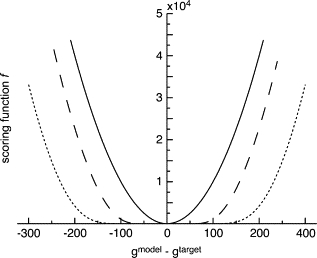
Examples of scoring functions with different parameters for values found in the PDF of the LAO binding protein (239 residues). (Solid line) simple-MSD scoring function; (dashed line) WMSD scoring function with the parameter ng^tar = 150; (dotted line) WMSD scoring function with ng^tar = 300. For a target PDF, g^tar, with a large value, the scoring function is flattened at the bottom, and thus less sensitive in the optimization process.

Elastic-network NMA

In our approach of flexible fitting, normal-mode vectors are used to deform the x-ray structure to ensure that the model structure is an energetically feasible conformation. The normal-mode method is based on the harmonic dynamics of the potential energy function around a minimum energy conformation (57) (see (58,59) for reviews). NMA first requires the Hessian matrix, L, which contains the second derivatives of the potential energy, V, at r = r⁰, where r⁰ is a minimum on the energy surface,

$$L_{\text{ij}}={\left(\frac{{\partial }^{2}V}{\partial r_{\text{i}}\partial r_{\text{j}}}\right|}_{\text{r}={\text{r}}^0}\text{.}$$

The dynamics of the system can be deduced by solving the eigenvalue problem to find vectors {a_n} that satisfy the equation

$${\text{M}}^{-1/2}\text{L}{\text{M}}^{-1/2}{\text{a}}_{\text{n}}={\omega }_{\text{n}}^2{\text{a}}_{\text{n}}$$

$${\text{a}}_{\text{n}}^{\text{T}}{\text{a}}_{\text{m}}={\delta }_{\text{n,m}},$$

where the matrix M contains atomic masses on its diagonal and δ_n,m is Kronecker's delta. The solution is a set of orthogonal eigenvectors, or normal modes, a_n = (a_1n, a_2n, …, a_3Nn)^T, and their associated frequencies, ω_n. The eigenvector gives the direction and relative amplitude of each atomic displacement. Using the normal modes, the dynamics of the system is described as a linear combination of independent harmonic oscillators (60).

We use a simplified representation of the potential energy function, which was first introduced by Tirion (35). This elastic network potential has been shown to be successful in reproducing large and collective motions of macromolecules. The potential energy of molecule is defined by:

$$V=\sum _{\text{i,j};{\text{d}}_{\text{ij}}^0<{\text{R}}_{\text{c}}}\frac{C}{2}(d_{\text{ij}}-d_{\text{ij}}^0),$$

where d_ij is the distance between atoms i and j; $d_{\text{ij}}^0$ is the distance in the given structure, and R_c is a cut-off parameter delimiting the distance beyond which elastic bonds are not included between atoms. R_c was set to 8 Å (33,36). As an additional coarse-graining, only Cα carbon atoms were considered. Several studies have shown that Cα carbons are sufficient to reproduce mechanical properties of the molecules (33,36–38). With the elastic network model, the developed methodology applies equally to Cα or the all-atoms model.

Each normal-mode vector represents a collective motion of the molecule. The modes with the lower frequencies represent preferential global motions (33). Thus, in the approach described here, we use the normal-mode coordinates associated with low-frequency normal mode as the optimization variables in place of Cartesian atomic coordinates. By limiting the deformation of the molecule along the low-frequency normal modes, we ensure that generated structural models are energetically accessible. In addition, by limiting the number of variables, i.e., normal-mode coordinates, to be optimized, we minimize the possibility of over-fitting. For applications of normal-mode refinement to 1D data, because the information embedded in the data is reduced compared to cryo-EM data, a smaller number of modes, 10, will be used in the refinement procedure. As it has been shown that typically one of the 10 lowest modes can represent functional motions (33), we should be able to characterize most of the conformational change using such an approach.

Iterative NMA

In NMA, the dynamics of the system is described as a combination of vibrational motions. Modes with low frequency can describe the large-scale conformational changes. When a structure is deformed along a mode l toward another structure, the amplitude of the deformation, q_l, that minimizes the root MSD (RMSD) between the target and deformed structures can be obtained by q_l = a_lΔr, where Δr represents the conformational difference between the two conformations and a_l is the mode vector of mode l. However, with such deformations, the quality of the generated model is not always optimal, as covalent bonds could have unphysical length. It occurs because conformational changes of biomolecules are anharmonic and nonlinear by nature, whereas normal modes only represent harmonic and linear motions.

To accurately describe conformational changes, one can take an iterative approach, i.e., a set of normal modes is used to generate only small deformations, and normal modes are recalculated for the slightly deformed structure (61–63). We define the initial conformation as C^I = (C⁰) and the final state as C^F. NMA is performed on C^t, with t initially taken as t = I. The structure, C^t, is displaced along a linear combination of normal modes, $a_l^{\text{t}},$ toward the final state, leading to the structure C^t+1. The deformation of the system is given by

$$x_{\text{n}}^{\text{t}+1}(\text{q})=\sum _{\text{l}=1}^{\text{M}}{a}_{\text{nl}}^{\text{t}}{q}_{\text{l}}^{\text{t}}+x_{\text{n}}^{\text{t}},$$ (2)

where $x_{\text{n}}^{\text{t}+1}(\text{q})$ and $x_{\text{n}}^{\text{t}}$ are the values of the coordinates of atom n after and before deformation, respectively; and M is the number of modes used to describe the transition. When the target is a 3D structure, the best magnitude of displacement along the mode l is given as

$$q_{\text{l}}^{\text{t}}={\text{a}}_{\text{l}}^{\text{t}}\cdot \Delta {\text{r}}^{\text{t}}Q,$$ (3)

where Δr^t is the vector difference between the current and target structures and Q modulates the magnitude of displacement so that the deformation at each iteration is small enough to accurately reproduce the nonlinear deformation. As demonstrated in the Results section, this iterative procedure can deform protein conformation from one to another using a small number of normal modes.

The best magnitude of displacement can be obtained from Eq. 3 only if both of the initial and target structures are provided. In the actual application of our algorithms the target is a PDF function. Thus, the amplitudes, {q_l}, need to be chosen in a way that the fitness of the deformed structure and the target PDF increases. In other words, we perform an optimization of scoring function with {q_l} as variables.

Optimization algorithm

When the fitting is performed using the iterative procedure, ideally the convergence should be achieved in a minimal number of iteration steps, since at each step the structure is deformed and distortions may accumulate in the structure. We need to identify a few normal modes that could deform the structure in such a way that it becomes more consistent with the experimental data. The efficiency of the algorithm depends on how well we identify the modes that produce deformations that are consistent with experimental data.

Steepest-descent and Newton Raphson methods

One of the standard approaches for optimization is to use gradient-following techniques such as steepest descent (SD), which was successfully implemented in the fitting with cryo-EM data (23). In this approach, the derivative of the scoring function with respect to normal-mode coordinates is computed and the displacement is made according to the value of the derivative. A large value means that the corresponding normal mode produces the steepest increase in the scoring function. Toward the end of the refinement, gradient-following techniques can fail, as curvature has more influence. Therefore, in the implementation with cryo-EM data, the final stage of the refinement optimization was performed according to an algorithm based on second derivatives, such as Newton Raphson, since it considers the curvature of the function surface (Hessian) and is more efficient when close to the maximum. This implementation was shown to be successful in refining high-resolution structure with low-resolution 3D data from cryo-EM.

Such a simple combination turns out to be not sufficient to identify normal modes that are relevant to conformational changes in the case of 1D data, since less information is contained within these data. Therefore, a more efficient optimization algorithm needs to be implemented, in which the second-derivative-based method is used in the earlier stages of the refinement to find the minimum in a smaller number of steps. However, a simple Newton Raphson method cannot be used from the beginning, since it gives the correct answer only when the original point is close to the minimum. In addition, we use an iterative normal-mode approach to reflect the nonlinear nature of the conformational change, and thus the calculated Hessian is considered to be accurate only within the structural deformation step size, which contradicts the approximation of the Newton-Raphson method.

Trusted region method

Therefore, to enhance the fitting efficiency, a new refinement procedure has been developed by incorporating a trusted region method (TRM) (64) with the Newton Raphson algorithm. This method was originally proposed to find the transition state for a chemical reaction and rely on the use of the Newton Raphson approach within a trusted region. Here, we propose to use this method for fitting the high-resolution structure of a biological molecule to low-resolution data.

In the TRM, one defines a radius within which the quadratic model equation is “trusted” to be a reasonable representation of the function (the simple Newton Raphson method trusts it for the entire space). Then, TRM tries to find the constrained minimum within the trusted region (Δ) using analytical formulas.

$$\text{max}\left\{f=\frac{1}{2}{\text{q}}^T\text{H}\text{q}+{\text{q}}^T\text{g}\text{such}\text{that}\parallel \text{q}\parallel <\Delta \right\},$$ (4)

where $\text{H}=\{{\partial }^{2}f/\partial q_{\text{l}}\partial q_{\text{m}}$} is the Hessian and $\text{g}=\{\partial f/\partial q_{\text{l}}\}$ the gradient. The amplitudes q = {q_l} that maximize f within the trusted region, Δ, are obtained using the Lagrange multiplier method. If the original point is sufficiently close to a minimum, then often the minimum lies within the circle of the trusted region and convergence is quite rapid, whereas near the start of a search, the constrained minimum will most likely lie on the boundary. Once the constrained minimum is found, we deform the structure using Eq. 2, with the amplitude q = {q_l} obtained by solving Eq. 4, and a new iteration begins. The process continues until convergence of f is observed. This method is conceptually well suited to the iterative normal mode, as in both we allow only limited movement.

To implement TRM into a refinement protocol, several sizes of the trusted region need to be tested to determine the optimal size. Indeed, too large a step size might lead to unrealistic deformations of the molecule and the quadratic approximation could fail. On the other hand, too small a step size would limit the efficiency of the program, as many steps would be needed to accomplish the transition.

Algorithm

The inputs of the refinement protocol are a PDF of a protein target structure and another high-resolution structure (x-ray or NMR) that the user wants to flexibly fit to the PDF data. NMA is first performed on the initial high-resolution structure using Cα atoms. Only the 10 lowest frequency normal modes are considered for the fitting. By limiting the number of modes included, one deforms the high-resolution structure without localized (bond/angle) distortion, which would be induced if higher-frequency modes were employed. In addition, limiting the dimensionality of the search decreases the time per iteration. Most importantly, the majority of the conformational change is generally captured using only the lowest-frequency normal modes (33).

After NMA on a high-resolution structure, s_n (n being the step number), is performed, the suitable normal-mode amplitudes for deformation are calculated by the SD method or by TRM. Theoretically, TRM should always be better than the SD method, and our results also confirm that. However, TRM requires the calculation of Hessian, which is time-consuming. Thus, at each step, we first estimate the best amplitudes for deformation by the SD method and deform the structure, obtaining s_n+1. If the score, f, between s_n+1 and the target PDF and the score expected from gradient analysis are in agreement within 5%, we accept the results from the SD method and keep s_n+1. If the actual score differs from the expected value by >5%, which indicates that the curvature of the function surface is not negligible, we reject the deformed structure, determine better amplitudes using TRM, and deform the structure accordingly, obtaining a new s_n+1. Modes are ranked according to the absolute value of the amplitude, and two or three of the vectors with the largest amplitudes are used for the deformation at each step. To avoid distortions of the structure, we limit the amount of deformation, i.e., the amplitude of normal mode, up to a 0.5-Å RMSD. Using such criteria ensures that the secondary structural motifs are conserved even after deformation.

We have tested two definitions for the scoring function, MSD and WMSD, in the above algorithm. In addition, two protocols of optimization termination have been tested. In the first protocol, the optimization is stopped when the score does not increase by iteration. In another protocol, the process is stopped when the increase of the score relative to its value has converged. The results show that the latter produces better fitting.

Algorithm testing procedure

To develop algorithms and evaluate their performance, we consider five proteins for which two distinctly different conformations are known from x-ray crystallography. For each protein, the PDF of one of two conformations is first generated. Then, starting from the other conformation, we apply our flexible fitting algorithms using the simulated PDF as the target. In this way, we are able to evaluate how the initial structure was deformed toward the target structure. As the fitting process progresses, the fitness (scoring function) of the deformed structure and the simulated target PDF improves. At the same time, we calculate the RMSDs of the deformed structure and the structure of the target. Ideally, when the scoring function reaches the maximum, the RMSD should reach a minimum. When RMSD decreases sufficiently as the fitting process proceeds, the algorithm can be considered to be working effectively.

We have tested five proteins: lysine/arginine/ornithine (LAO) binding protein (2lao and 1lst), adenylate kinase (4ake and 1ake), maltodextrin binding protein (1omp and 1anf), lactoferrin (1lfg and 1lfh), and elongation factor 2 (1n0u and 1n0v). These proteins differ from each other in size, shape, and magnitude of conformational transition, and are useful for observing the applicability of our new algorithm to a variety of proteins.

In this article, we present only results using coarse-grained—Cα atoms—elastic-network NMA but we should note that the same results are obtained using the all-atoms elastic-network NMA (data not shown).

Results

Evaluating the best performance of the iterative normal-mode approach

Before we perform the flexible fitting procedure from an x-ray structure to the PDF, we first test a fitting from an x-ray structure to another x-ray structure using the optimization algorithms described above. The original structure is deformed toward the target structure by iterative NMA using Eq. 2, with the displacement amplitude given by Eq. 3. This analysis will exhibit how the flexible fitting could potentially work in the best-case scenario, i.e., where a high-resolution structure is known for the two end points. These data illustrate the upper limit, in terms of RMSD, that we could obtain for the newly proposed method. Fig. 2 illustrates the use of the iterative normal mode for structure deformation toward a known x-ray structure displaying a different conformation. The RMSD as a function of the iteration step, t, between C^t and C^F is shown for four proteins. In these examples, only the 10 lowest-frequency normal modes were computed at each step, and three modes were used for deformation. The RMSD between C^t and C^F can be reduced to <2 Å for each protein and to as low as 1 Å for the LAO binding protein. Such data show that it is not necessary to have a large number of modes to represent most of the large collective conformational changes of a biological molecule. Rather, only a few modes, e.g., three, can be used to obtain a final RMSD that is within the limit of the resolution of the low-resolution experimental data. Obviously, when the fitting is performed with lower-resolution data, higher RMSD values are expected. Such an approach was successfully implemented with cryo-EM data, which contains low-resolution 3D data. These final RMSDs represent the best values that can be obtained in such specific conditions. These values depend primarily on how well the normal modes can describe the conformational change between the two known structures. Fitting with low-resolution data will only result in higher RMSDs, as the definition of the target structure contains less information.

Figure 2.

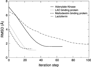
Performance of iterative NMA from 3D structure to 3D structure for four proteins. For each protein, the algorithm successfully deforms the structure very close to the target structure.

LAO binding protein

In the above analysis, the conformational change of the LAO binding protein was most successfully simulated by iterative NMA. Thus, we choose the LAO binding protein as the first test case of the fitting from x-ray structure to PDF. The difference between the two conformations of the LAO binding protein has an ∼5-Å RMSD. From one of the conformations, a PDF was generated and used as the target to test our algorithms.

We ran four different optimization procedures using either a simple SD approach or an approach using a combination of SD and TRM, and for each run two different scoring functions were used, MSD or WMSD.

Although we can observe a decrease in the RMSD in all cases (Fig. 3), it is difficult to determine at what point the value of the score has converged. Indeed, the scoring function continuously increases, even though the RMSD might reincrease as well, i.e., nonnecessary protein deformation might occur. We observed these phenomena using both scoring functions. In some cases, the additional RMSD increase reverts back to 5 Å after reaching a minimum of 2.4 Å.

Figure 3.

Progress of the fitting process for the LAO binding protein measured by fitness scoring function and RMSD. Combinations of two scoring functions, simple MSD and WMSD, and two optimization methods, SD and TRM, are tested. The progress of the RMSD is shown as solid lines and the scoring functions as broken lines. The best model, which is closest to the target structure, is obtained by the combination of WMSD and TRM.

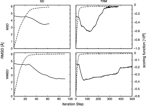
Therefore, we decided to investigate another criterion to define convergence of the optimization process. Rather than looking directly at the value of the scoring function, we calculated the relative change of the score, f, from step i and step i + 1. Fig. 4 shows the trajectory of the relative change over the fitting process. For the fitting process with TRM/MSD, the relative change in the score is not close to zero even after the best fitting has been obtained. When it reaches zero, the structure is already deformed repeatedly from the best structure, which results in increases of the RMSD. Using the relative change in the score value in conjunction with the WMSD scoring function, we can clearly see that the relative change reaches zero when the structure is deformed optimally in terms of the RMSD. Therefore, we use such a variable as a criterion to stop the optimization.

Figure 4.

Progress of RMSD and relative change in the scoring function over the fitting process for the LAO binding protein. As in Fig. 3, a combination of the two scoring functions, simple MSD and WMSD, and two optimization methods, SD and TRM, are tested. The progress of the RMSD is shown by solid lines and the relative change of scoring functions by dashed lines. The relative change reaches zero when the RMSD is close to the minimum.

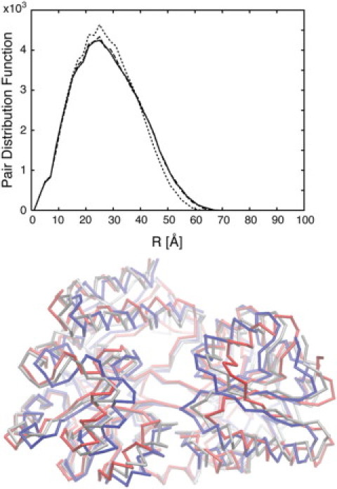
The model obtained from our algorithm using WMSD in conjunction with TRM is shown in Fig. 5, along with the starting structure and the answer, i.e., the source of the target PDF. In addition, the PDFs of three conformations are shown for comparison. The result shows that the conformational change of the LAO binding protein, i.e., closing of the two domains to isolate the active site, has been successfully reproduced by the fitting to the PDF data.

Figure 5.

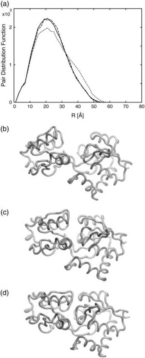
(a) The PDFs of initial (dotted line), predicted (dashed line), and target (solid line) structures are shown. (b–d). The initial structure of the LAO binding protein (b), the modeled structure predicted from the fitting algorithm (c), and the structure from which the target PDF is created (d). The PDF of the predicted structure is in close agreement with the target PDF and the structures are also very similar.

Tests for other proteins

Using the relative change in the score value as the convergence parameter, additional fitting processes were performed on several proteins. We tested the algorithm using either the MSD or WMSD scoring function and both optimization algorithms. For each protein, different numbers of modes (two or three) were also used for displacement of the structure. In addition, several radii for the TRM and SD displacements were tested. The results for all proteins tested are shown in Table 1.

Table 1.

Results of tests using different scoring functions and optimization algorithms

			Proteins
	Displacement	Number of modes	Adenylate kinase	Elongation factor 2	LAO binding protein	Lactoferrin	Maltodextrin binding protein
	Initial RMSD		7.2	14.6	4.8	6.6	4.0
MSD
RMSD	r = 0.1	2	3.6	fails	3.6	5.7	fails
			2.5	14.3	2.5	6.9	2.6
		3	3.6	fails	3.1	5.7	3.4
			3.8	fails	2.5	6.7	2.6
	r = 0.3	2	2.9	14.41	4.0	5.7	3.9
			2.6	fails	3.4	6.1	2.5
		3	3.8	fails	3.6	5.6	3.5
			3.7	fails	2.8	3.1	2.7
WMSD
RMSD	r = 0.1	2	3.8	9.1	2.5	5.6	3.3
			2.8	5.7	2.4	4.2	3.4
		3	4.3	10.9	3.1	5.6	3.3
			4.4	6.3	2.3	4.0	3.2
	r = 0.3	2	3.8	9.6	3.6	6.2	4.0
			3.0	5.7	3.0	5.6	4.0
		3	3.9	12.1	3.9	5.8	3.4
			4.3	6.0	2.9	4.5	3.3

Data displayed in regular weight are from the SD optimization, and data in bold are from the TRM optimization. r, radius of the trusted region method used in the refinement; (fails) the optimization process failed to decrease the RMSD.

Overall, the RMSD is decreased for all proteins when the WMSD is used. With the MSD scoring function, decrease of the RMSD is also observed for some proteins. However, in the case of elongation factor 2, which displays the largest conformational change, the refinement fails almost consistently. Therefore, it is preferable to use the WMSD, which can reduce the RMSD for all proteins tested.

We note that using two modes with the WMSD scoring function with a radius of 0.1 Å for the displacement produces the best fitting overall. Increasing the size of amplitude of displacement leads to less accurate results. TRM gives better results in general compared to the simple SD algorithm. Thus, incorporating information about the second derivative provides a better result.

Discussion

Choice of optimization algorithm: SD/TRM

A clear indication of how TRM works can be seen from Fig. 4. The relative change of the score as a function of step is relatively smooth toward the end of the algorithm compared to when SD is used. Indeed, a major difference between SD and TRM is that even though we assign a certain radius for protein deformation, TRM can find a conformation with the maximum score within the radius; therefore, the overall displacement of the protein may be less than the maximum radius. The results also reveal that at a certain point during the refinement (especially pronounced in the case of the MSD), the gradient method starts to fail, whereas with TRM the RMSD continues to decrease. At the beginning of the refinement, the gradient is a good way to optimize the scoring function. However, as we come closer to the target, the contribution from the second derivative becomes more important, and the gradient is not sufficient at that point.

Choice of radius for trusted region method

We ran simulations with several trusted-region radii. In each case, it appears that a smallest value gives better results. We should note that the structure is of good quality as a result of the iterative normal-mode approach. Indeed, by setting a maximum deviation of 0.1 Å overall for the protein, most of the distortions are avoided during the refinement. Using larger radii decreases the accuracy of the fitting, and in such cases, e.g., with a radius of 0.5 Å, in some proteins we observed unusual Cα-Cα distances, which are due to too-large deformations at a single step (data not shown). We should note that using a smaller radius increases the number of iteration steps, and therefore although it is more accurate, the refinement procedure takes longer time.

Limitation to fitting 1D data

The results indicate that for most proteins we can predict the conformation within an RMSD of ∼2–3 Å, which in terms of accuracy is close to what can be observed for structures obtained from homology modeling. The obtained model for the elongation factor agrees least with the target (final RMSD ∼5 Å). However, it is a significant improvement over the original conformational difference, which was very large (∼15 Å). In addition, most of the conformational change is described correctly thanks to the fitting process. For two proteins, the maltodextrin binding protein and lactoferrin, the accuracy is less than ideal in comparison to the original RMSD. In fact, we note that the difference in the PDF profiles between the two conformations is rather small, which may indicate some limitation to fitting low-resolution data. Fig. 6 shows the initial, target, and modeled structures of maltodextrin binding protein, as well as their corresponding PDFs. The difference between the PDFs of the initial and target structures is relatively small compared to that of the LAO binding protein (Fig. 5), which would explain the poor performance in the fitting of maltodextrin binding protein. To identify the normal modes that reproduce the conformational change, the difference between the PDFs needs to be large enough.

Figure 6.

(Upper) The PDFs of the initial (dotted line), target (solid line), and constructed model (dashed line). (Lower) The initial structure of the maltodextrin binding protein (red), the structure from which the target PDF is created (blue), and the modeled structure predicted from the fitting algorithm (silver) are shown. For this system, since the difference between the initial and target PDFs is small, the modeled structure does not exactly agree with the target structure; however, trends of the conformational change are predicted.

Nevertheless, we should note that even though the structure is not very accurate, the final conformation displays some of the characteristics of the conformational change. Indeed, in the case of the maltodextrin binding protein, comparison of the initial, final, and predicted conformations shows that the predicted structure lies between the other two conformations (Fig. 6). The displacement obtained from the fitting points in the good direction; however, there is not sufficient information from the low-resolution data to fully reproduce the full conformational change. It indicates that even though our approach may fail to construct a model close to the final structure, insights on the directionality of conformational changes can be reliably obtained.

Conclusion

We have presented a new algorithm to reconstruct an atomic level structure from an atomic pair distribution function. This new algorithm takes advantage of an already known x-ray structure to predict a different conformation embedded in the pair distribution function. Normal-mode theory is used to construct a model by deforming the original x-ray structure to ensure that the new conformation is energetically accessible. Using simulated 1D data, we have demonstrated that our approach makes it possible to predict directions of conformational changes and to construct structures within 3 Å of the target data. Such an approach should prove useful in interpreting low-resolution 1D data.

We choose the pair distribution function as an example of very low dimensional data. PDF data is 1D and thus provides far less information than 3D structural data obtained from techniques such as cryo-EM. The theories behind the method, as well as an example for a small protein, have been introduced in this article, and we have shown that our protocol is successful in predicting structure from 1D data. We intend to extend this methodology for fitting experimental data derived from SAXS data, which is also 1D. In the case of SAXS, the influence of the solvent needs to be considered, and experimental error also needs to be included. Results of that work will be presented in a separate article.

References

- 1.Saibil H.R. Conformational changes studied by cryo-electron microscopy. Nat. Struct. Biol. 2000;7:711–714. doi: 10.1038/78923. [DOI] [PubMed] [Google Scholar]
- 2.Heller W.T., Vigil D., Brown S., Blumenthal D.K., Taylor S.S., Trewhella J. C subunits binding to the protein kinase A RIα dimer induce a large conformational change. J. Biol. Chem. 2004;279:19084–19090. doi: 10.1074/jbc.M313405200. [DOI] [PubMed] [Google Scholar]
- 3.Priddy T.S., Macdonald B.A., Heller W.T., Nadeau O.W., Trewhella J., Carlson G.M. Ca2+-induced structural changes in phosphorylase kinase detected by small-angle X-ray scattering. Protein Sci. 2005;14:1039–1048. doi: 10.1110/ps.041124705. [DOI] [PMC free article] [PubMed] [Google Scholar]
- 4.Vestergaard B., Sanyal S., Roessle M., Mora L., Buckingham R.H., Kastrup J.S., Gajhede M., Svergun D.I., Ehrenberg M. The SAXS solution structure of RF1 differs from its crystal structure and is similar to its ribosome bound cryo-EM structure. Mol. Cell. 2005;20:929–938. doi: 10.1016/j.molcel.2005.11.022. [DOI] [PubMed] [Google Scholar]
- 5.Ermolenko D.N., Spiegel P.C., Majumdar Z.K., Hickerson R.P., Clegg R.M., Noller H.F. The antibiotic viomycin traps the ribosome in an intermediate state of translocation. Nat. Struct. Mol. Biol. 2007;14:493–497. doi: 10.1038/nsmb1243. [DOI] [PubMed] [Google Scholar]
- 6.Hickerson R., Majumdar Z.K., Baucom A., Clegg R.M., Noller H.F. Measurement of internal movements within the 30 S ribosomal subunit using Forster resonance energy transfer. J. Mol. Biol. 2005;354:459–472. doi: 10.1016/j.jmb.2005.09.010. [DOI] [PubMed] [Google Scholar]
- 7.Majumdar Z.K., Hickerson R., Noller H.F., Clegg R.M. Measurements of internal distance changes of the 30 S ribosome using FRET with multiple donor-acceptor pairs: quantitative spectroscopic methods. J. Mol. Biol. 2005;351:1123–1145. doi: 10.1016/j.jmb.2005.06.027. [DOI] [PubMed] [Google Scholar]
- 8.Hammel M., Fierober H.P., Czjzek M., Kurkal V., Smith J.C., Bayer E.A., Finet S., Receveur-Brechot V. Structural basis of cellulosome efficiency explored by small angle X-ray scattering. J. Biol. Chem. 2005;280:38562–38568. doi: 10.1074/jbc.M503168200. [DOI] [PubMed] [Google Scholar]
- 9.Aramayo R., Merigoux C., Larquet E., Bron P., Perez J., Dumas C., Vachette P., Boisset N. Divalent ion-dependent swelling of tomato bushy stunt virus: a multi-approach study. Biochim. Biophys. Acta. 2005;1724:345–354. doi: 10.1016/j.bbagen.2005.05.020. [DOI] [PubMed] [Google Scholar]
- 10.Fabiola F., Chapman M.S. Fitting of high-resolution structures into electron microscopy reconstruction images. Structure. 2005;13:389–400. doi: 10.1016/j.str.2005.01.007. [DOI] [PubMed] [Google Scholar]
- 11.Wriggers W., Birmanns S. Using Situs for flexible and rigid-body fitting of multiresolution single-molecule data. J. Struct. Biol. 2001;133:193–202. doi: 10.1006/jsbi.2000.4350. [DOI] [PubMed] [Google Scholar]
- 12.Petoukhov M.V., Svergun D.I. Global rigid body modeling of macromolecular complexes against small-angle scattering data. Biophys. J. 2005;89:1237–1250. doi: 10.1529/biophysj.105.064154. [DOI] [PMC free article] [PubMed] [Google Scholar]
- 13.Zheng W., Doniach S. Fold recognition aided by constraints from small angle X-ray scattering data. Protein Eng. Des. Sel. 2005;18:209–219. doi: 10.1093/protein/gzi026. [DOI] [PubMed] [Google Scholar]
- 14.Wu Y.H., Tian X., Lu M.Y., Chen M.Z., Wang Q.H., Ma J.P. Folding of small helical proteins assisted by small-angle X-ray scattering profiles. Structure. 2005;13:1587–1597. doi: 10.1016/j.str.2005.07.023. [DOI] [PubMed] [Google Scholar]
- 15.Walther D., Cohen F.E., Doniach S. Reconstruction of low-resolution three-dimensional density maps from one-dimensional small-angle X-ray solution scattering data for biomolecules. J. Appl. Crystallogr. 2000;33:350–363. [Google Scholar]
- 16.Topf M., Sali A. Combining electron microscopy and comparative protein structure modeling. Curr. Opin. Struct. Biol. 2005;15:578–585. doi: 10.1016/j.sbi.2005.08.001. [DOI] [PubMed] [Google Scholar]
- 17.Mears J.A., Sharma M.R., Gutell R.R., McCook A.S., Richardson P.E., Caulfield T.R., Agrawal R.K., Harvey S.C. A structural model for the large subunit of the mammalian mitochondrial ribosome. J. Mol. Biol. 2006;358:193–212. doi: 10.1016/j.jmb.2006.01.094. [DOI] [PMC free article] [PubMed] [Google Scholar]
- 18.Chacon P., Diaz J.F., Moran F., Andreu J.M. Reconstruction of protein form with X-ray solution scattering and a genetic algorithm. J. Mol. Biol. 2000;299:1289–1302. doi: 10.1006/jmbi.2000.3784. [DOI] [PubMed] [Google Scholar]
- 19.Volkmann N., Hanein D., Ouyang G., Trybus K.M., DeRosier D.J., Lowey S. Evidence for cleft closure in actomyosin upon ADP release. Nat. Struct. Biol. 2000;7:1147–1155. doi: 10.1038/82008. [DOI] [PubMed] [Google Scholar]
- 20.Wendt T., Taylor D., Trybus K.M., Taylor K. Three-dimensional image reconstruction of dephosphorylated smooth muscle heavy meromyosin reveals asymmetry in the interaction between myosin heads and placement of subfragment 2. Proc. Natl. Acad. Sci. USA. 2001;98:4361–4366. doi: 10.1073/pnas.071051098. [DOI] [PMC free article] [PubMed] [Google Scholar]
- 21.Rawat U.B.S., Zavialov A.V., Sengupta J., Valle M., Grassucci R.A., Linde J., Vestergaard B., Ehrenberg M., Frank J. A cryo-electron microscopic study of ribosome-bound termination factor RF2. Nature. 2003;421:87–90. doi: 10.1038/nature01224. [DOI] [PubMed] [Google Scholar]
- 22.Reference deleted in proof.
- 23.Tama F., Miyashita O., Brooks C.L., III Flexible multi-scale fitting of atomic structures into low-resolution electron density maps with elastic network normal mode analysis. J. Mol. Biol. 2004;337:985–999. doi: 10.1016/j.jmb.2004.01.048. [DOI] [PubMed] [Google Scholar]
- 24.Go N., Noguti T., Nishikawa T. Dynamics of a small globular protein in terms of low-frequency vibrational modes. Proc. Natl. Acad. Sci. USA. 1983;80:3696–3700. doi: 10.1073/pnas.80.12.3696. [DOI] [PMC free article] [PubMed] [Google Scholar]
- 25.Brooks B.R., Karplus M. Harmonic dynamics of proteins: normal mode and fluctuations in bovine pancreatic trypsin inhibitor. Proc. Natl. Acad. Sci. USA. 1983;80:6571–6575. doi: 10.1073/pnas.80.21.6571. [DOI] [PMC free article] [PubMed] [Google Scholar]
- 26.Harrison W. Variational calculation of the normal modes of a large macromolecule: methods and some initial results. Biopolymers. 1984;23:2943–2949. doi: 10.1002/bip.360231216. [DOI] [PubMed] [Google Scholar]
- 27.Brooks B.R., Karplus M. Normal modes for specific motions of macromolecules: application to the hinge-bending mode of lysozyme. Proc. Natl. Acad. Sci. USA. 1985;82:4995–4999. doi: 10.1073/pnas.82.15.4995. [DOI] [PMC free article] [PubMed] [Google Scholar]
- 28.Gibrat J.F., Go N. Normal mode analysis of human lysozyme: study of the relative motion of the two domains and characterization of the harmonic motion. Proteins. 1990;8:258–279. doi: 10.1002/prot.340080308. [DOI] [PubMed] [Google Scholar]
- 29.Seno Y., Go N. Deoxymyoglobin studied by the conformational normal mode analysis. 1. Dynamics of globin and the heme-globin interaction. J. Mol. Biol. 1990;216:95–109. doi: 10.1016/S0022-2836(05)80063-4. [DOI] [PubMed] [Google Scholar]
- 30.Perahia D., Mouawad L. Computation of low-frequency normal modes in macromolecules: improvements to the method of diagonalization in a mixed basis and application to hemoglobin. Comput. Chem. 1995;19:241–246. doi: 10.1016/0097-8485(95)00011-g. [DOI] [PubMed] [Google Scholar]
- 31.Mouawad L., Perahia D. Motions in hemoglobin studied by normal mode analysis and energy minimization: evidence for the existence of tertiary T-like, quaternary R-like intermediate structures. J. Mol. Biol. 1996;258:393–410. doi: 10.1006/jmbi.1996.0257. [DOI] [PubMed] [Google Scholar]
- 32.Delarue M., Sanejouand Y.H. Simplified normal mode analysis of conformational transitions in DNA-dependent polymerases: the elastic network model. J. Mol. Biol. 2002;320:1011–1024. doi: 10.1016/s0022-2836(02)00562-4. [DOI] [PubMed] [Google Scholar]
- 33.Tama F., Sanejouand Y.H. Conformational change of proteins arising from normal mode calculations. Protein Eng. 2001;14:1–6. doi: 10.1093/protein/14.1.1. [DOI] [PubMed] [Google Scholar]
- 34.Nicolay S., Sanejouand Y.H. Functional modes of proteins are among the most robust. Phys. Rev. Lett. 2006;96:078104. doi: 10.1103/PhysRevLett.96.078104. [DOI] [PubMed] [Google Scholar]
- 35.Tirion M.M. Large amplitude elastic motions in proteins from a single- parameter, atomic analysis. Phys. Rev. Lett. 1996;77:1905–1908. doi: 10.1103/PhysRevLett.77.1905. [DOI] [PubMed] [Google Scholar]
- 36.Bahar I., Atilgan A.R., Erman B. Direct evaluation of thermal fluctuations in proteins using a single-parameter harmonic potential. Fold. Des. 1997;2:173–181. doi: 10.1016/S1359-0278(97)00024-2. [DOI] [PubMed] [Google Scholar]
- 37.Hinsen K. Analysis of domain motions by approximate normal mode calculations. Proteins. 1998;33:417–429. doi: 10.1002/(sici)1097-0134(19981115)33:3<417::aid-prot10>3.0.co;2-8. [DOI] [PubMed] [Google Scholar]
- 38.Doruker P., Jernigan R.L., Bahar I. Dynamics of large proteins through hierarchical levels of coarse-grained structures. J. Comput. Chem. 2002;23:119–127. doi: 10.1002/jcc.1160. [DOI] [PubMed] [Google Scholar]
- 39.Bahar I., Rader A.J. Coarse-grained normal mode analysis in structural biology. Curr. Opin. Struct. Biol. 2005;15:586–592. doi: 10.1016/j.sbi.2005.08.007. [DOI] [PMC free article] [PubMed] [Google Scholar]
- 40.Tama F., Brooks C.L., III The mechanism and pathway of pH induced swelling in cowpea chlorotic mottle virus. J. Mol. Biol. 2002;318:733–747. doi: 10.1016/S0022-2836(02)00135-3. [DOI] [PubMed] [Google Scholar]
- 41.Tama F., Valle M., Frank J., Brooks C.L., III Dynamic reorganization of the functionally active ribosome explored by normal mode analysis and cryo-electron microscopy. Proc. Natl. Acad. Sci. USA. 2003;100:9319–9323. doi: 10.1073/pnas.1632476100. [DOI] [PMC free article] [PubMed] [Google Scholar]
- 42.Rader A.J., Vlad D.H., Bahar I. Maturation dynamics of bacteriophage HK97 capsid. Structure. 2005;13:413–421. doi: 10.1016/j.str.2004.12.015. [DOI] [PubMed] [Google Scholar]
- 43.Wang Y.M., Rader A.J., Bahar I., Jernigan R.L. Global ribosome motions revealed with elastic network model. J. Struct. Biol. 2004;147:302–314. doi: 10.1016/j.jsb.2004.01.005. [DOI] [PubMed] [Google Scholar]
- 44.Tama F., Wriggers W., Brooks C.L., III Exploring global distortions of biological macromolecules and assemblies from low-resolution structural information and elastic network theory. J. Mol. Biol. 2002;321:297–305. doi: 10.1016/s0022-2836(02)00627-7. [DOI] [PubMed] [Google Scholar]
- 45.Chacon P., Tama F., Wriggers W. Mega-Dalton biomolecular motion captured from electron microscopy reconstructions. J. Mol. Biol. 2003;326:485–492. doi: 10.1016/s0022-2836(02)01426-2. [DOI] [PubMed] [Google Scholar]
- 46.Ming D., Kong Y.F., Lambert M.A., Huang Z., Ma J.P. How to describe protein motion without amino acid sequence and atomic coordinates. Proc. Natl. Acad. Sci. USA. 2002;99:8620–8625. doi: 10.1073/pnas.082148899. [DOI] [PMC free article] [PubMed] [Google Scholar]
- 47.Ming D.M., Kong Y.F., Wakil S.J., Brink J., Ma J.P. Domain movements in human fatty acid synthase by quantized elastic deformational model. Proc. Natl. Acad. Sci. USA. 2002;99:7895–7899. doi: 10.1073/pnas.112222299. [DOI] [PMC free article] [PubMed] [Google Scholar]
- 48.Kidera A., Go N. Refinement of protein dynamic structure: normal mode refinement. Proc. Natl. Acad. Sci. USA. 1990;87:3718–3722. doi: 10.1073/pnas.87.10.3718. [DOI] [PMC free article] [PubMed] [Google Scholar]
- 49.Kidera A., Go N. Normal mode refinement: crystallographic refinement of protein dynamic structure. 1. Theory and test by simulated diffraction data. J. Mol. Biol. 1992;225:457–475. doi: 10.1016/0022-2836(92)90932-a. [DOI] [PubMed] [Google Scholar]
- 50.Kidera A., Inaka K., Matsushima M., Go N. Normal mode refinement: crystallographic refinement of protein dynamic structure. 2. Application to human lysozyme. J. Mol. Biol. 1992;225:477–486. doi: 10.1016/0022-2836(92)90933-b. [DOI] [PubMed] [Google Scholar]
- 51.Tama F., Miyashita O., Brooks C.L., III NMFF: flexible high-resolution annotation of low-resolution experimental data from cryo-EM maps using normal mode analysis. J. Struct. Biol. 2004;147:315–326. doi: 10.1016/j.jsb.2004.03.002. [DOI] [PubMed] [Google Scholar]
- 52.Mitra K., Schaffitzel C., Shaikh T., Tama F., Jenni S., Brooks C.L., III, Ban N., Frank J. Structure of the E. coli protein-conducting channel bound to a translating ribosome. Nature. 2005;438:318–324. doi: 10.1038/nature04133. [DOI] [PMC free article] [PubMed] [Google Scholar]
- 53.Delarue M., Dumas P. On the use of low-frequency normal modes to enforce collective movements in refining macromolecular structural models. Proc. Natl. Acad. Sci. USA. 2004;101:6957–6962. doi: 10.1073/pnas.0400301101. [DOI] [PMC free article] [PubMed] [Google Scholar]
- 54.Hinsen K., Reuter N., Navaza J., Stokes D.L., Lacapere J.J. Normal mode-based fitting of atomic structure into electron density maps: Application to sarcoplasmic reticulum Ca-ATPase. Biophys. J. 2005;88:818–827. doi: 10.1529/biophysj.104.050716. [DOI] [PMC free article] [PubMed] [Google Scholar]
- 55.Petoukhov M.V., Svergun D.I. New methods for domain structure determination of proteins from solution scattering data. J. Appl. Cryst. 2003;36:540–544. [Google Scholar]
- 56.Svergun D.I., Koch M.H.J. Small-angle scattering studies of biological macromolecules in solution. Rep. Prog. Phys. 2003;66:1735–1782. [Google Scholar]
- 57.Goldstein H. Addison-Wesley; Stamford, CT: 1950. Classical Mechanics. [Google Scholar]
- 58.Case D.A. Normal-mode analysis of protein dynamics. Curr. Opin. Struct. Biol. 1994;4:285–290. [Google Scholar]
- 59.Ma J.P. Usefulness and limitations of normal mode analysis in modeling dynamics of biomolecular complexes. Structure. 2005;13:373–380. doi: 10.1016/j.str.2005.02.002. [DOI] [PubMed] [Google Scholar]
- 60.Brooks C.L., III, Karplus M., Pettit B.M. Wiley; New York: 1988. Proteins: A Theoretical Perspertive of Dynamics, Structure and Thermodynamics. [Google Scholar]
- 61.Tama F., Feig M., Liu J., Brooks C.L., III, Taylor K.A. The requirement for mechanical coupling between head and S2 domains in smooth muscle myosin ATPase regulation and its implications for dimeric motor function. J. Mol. Biol. 2005;345:837–854. doi: 10.1016/j.jmb.2004.10.084. [DOI] [PubMed] [Google Scholar]
- 62.Miyashita O., Onuchic J.N., Wolynes P.G. Nonlinear elasticity, proteinquakes, and the energy landscapes of functional transitions in proteins. Proc. Natl. Acad. Sci. USA. 2003;100:12570–12575. doi: 10.1073/pnas.2135471100. [DOI] [PMC free article] [PubMed] [Google Scholar]
- 63.Miyashita O., Wolynes P.G., Onuchic J.N. Simple energy landscape model for the kinetics of functional transitions in proteins. J. Phys. Chem. B. 2005;109:1959–1969. doi: 10.1021/jp046736q. [DOI] [PubMed] [Google Scholar]
- 64.Cerjan C.J., Miller W.H. On finding transition-states. J. Chem. Phys. 1981;75:2800–2806. [Google Scholar]