Statistical analysis of shape through triangulation of landmarks: A study of sexual dimorphism in hominids

Abstract

Two objects with homologous landmarks are said to be of the same shape if the configuration of landmarks of one object can be exactly matched with that of the other by translation, rotation/reflection, and scaling. In an earlier paper, the authors proposed statistical analysis of shape by considering logarithmic differences of all possible Euclidean distances between landmarks. Tests of significance for differences in the shape of objects and methods of discrimination between populations were developed with such data. In the present paper, the corresponding statistical methodology is developed by triangulation of the landmarks and by considering the angles as natural measurements of shape. This method is applied to the study of sexual dimorphism in hominids.

1. Introduction

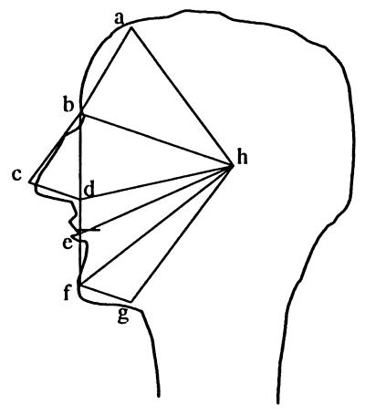
In a previous paper (1), the authors presented a statistical analysis of the shape of objects considering the ratios of Euclidean distances between landmarks as basic data. As observed by Lele (2), such ratios, which are invariant to translation, rotation, and scaling of the configuration of landmarks, provide measurements on shape. If there are k landmarks, we have a set of k(k − 1)/2 Euclidean distances, all of which may not be necessary to specify the configuration of landmarks on an object. We suggested the choice of a minimal set of distances that uniquely specify the configuration of landmarks for purposes of statistical inference. For a two-dimensional object with k landmarks, this number lies between (2k − 3) and 3(k − 2). In general, when the relative positions of landmarks are known, (2k − 3) distances will do, as in the case of the human profile illustrated in our earlier paper and reproduced below (Fig. 1). There are 8 landmarks indicated by a, b, c, d, e, f, g, and h, with 28 distances between landmarks. However, 13 distances, as indicated in Fig. 1, specify the entire configuration.

Figure 1.

Minimum number of distances required to fix the landmarks on human facial profile. (Modified from ref. 1.)

It may be seen from the above diagram that the configuration of landmarks can also be specified by 6 triangles. Each triangle provides two angles that are invariant to translation, rotation, and scaling. There are altogether 12 angles arising out of 6 triangles, which appear to be natural shape measurements. We explore the possibility of studying differences in shape through angular coordinates resulting from a suitable triangulation of the landmarks. Such an approach was also indicated by Bookstein (3), although he did not develop the appropriate statistical methodology.

We shall first discuss the simple case of three landmarks and suggest a general approach in the case of many landmarks.

We also discuss the possibility of augmenting the angular data provided by a triangulation of the landmarks with sets of angles characterizing the shape of the edges (or profiles), if available, between landmarks. Such data may provide additional information in problems of discrimination and identification of objects by shape.

2. Objects Specified by Three Landmarks

First, we consider objects specified by three landmarks, say 1, 2, and 3, and denote the angles at the corresponding vertices by θ₁, θ₂, and θ₃, which add up to 180 degrees (or π radians). These angles, which are natural measurements of shape, are referred to in statistical literature as compositional data. For purposes of statistical inference, one may choose a suitable stochastic model and apply the appropriate methodology for estimation and tests of significance. For a discussion of some models for compositional data, the reader is referred to a book by Aitchison (4) and a paper by Pukkila and Rao (5). It may be noted that because θ₁, θ₂, and θ₃ are non-negative, they can be transformed to directional data by considering l_i = , i = 1, 2, 3, in which case an appropriate stochastic model for directional data may be used. See Mardia (6) and Pukkila and Rao (5) for a discussion of models for directional data and statistical inference based on them. Alternatively, one can use nonparametric methods.

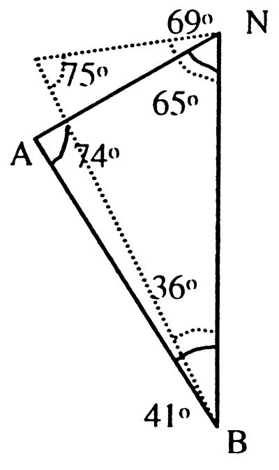
For purpose of illustration, we use the angular data (in degrees) given in Aitchison (ref. 4, pp. 385–386) relating to three landmarks, nasion (N), alveolar (A), and basion (B), on seventeenth century English and Naqada skulls. The mean values of the angles designated as N, A, and B and the sample sizes (in parentheses) for male and female skulls are given in Table 1. The pooled sums of squares and products are given in Table 2.

Table 1.

Mean values of the three angles for English and Naqada skulls

θ	English			Naqada
	Male (29)	Female (22)	Combined (51)	Male (29)	Female (22)	Combined (51)
N	65.241	64.750	65.029	69.579	69.389	69.497
A	73.707	73.705	73.706	74.452	75.361	74.844
B	41.052	41.591	41.284	35.976	35.250	35.663

Table 2.

Pooled sums of squares and products matrices (degrees of freedom = 98)

N	A	B
1490.213	−1321.989	−168.949
−1321.989	1636.930	−316.016
−168.949	−316.016	487.759

Because the sum of the angles is a constant, we need consider only two angles. We choose N and A. A new test for multivariate normality (bivariate in the present problem) developed by Rao and Ali (7) had p-values of the order of 0.75 for English and 0.29 for Naqada data (with possibly one or two outliers in the latter case) showing no significant departure from normality. In case non-normality is indicated, we may try transformations such as

whose distributions may be close to bivariate normality than θ₁ and θ₂. Table 3 gives the Hotelling T² values for testing differences between male and female skulls in English and Naqada skulls and also differences between groups ignoring sex. The formula for T² is

where n₁ and n₂ are sample sizes for two groups under comparison, n is the degrees of freedom (98 in our case) for S as in Table 2, p is the number of variables (2 in our case), d is the vector of differences in mean values, and S⁻¹ is the inverse of S. Under the normality assumption, T² has an F distribution with p and (n − p + 1) degrees of freedom.

Table 3.

Tests of hypotheses based on the angles N and A

Skulls	Hotelling’s T2	d.f. for F	p-values
English (male − female)	0.349	2, 97	0.706
Naqada (male − female)	0.731	2, 97	0.483
English − Naqada (ignoring sex)	85.908	2, 97	0.000

It is seen that there are no differences in the shapes of male and female skulls within a group. However, the shapes of English and Naqada skulls are different. The mean shapes of triangles formed by N, A, B for the English and Naqada skulls are represented in Fig. 2.

Figure 2.

Mean shapes of English (thick line) and Naqada (dotted line) triangles.

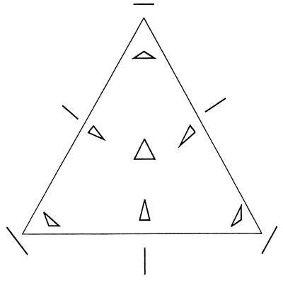
The angles for an individual can be represented with aerial coordinates within an equilateral triangle. The shapes of triangles represented by points in different positions within the equilateral triangle are shown in Fig. 3.

Figure 3.

Shapes of triangles corresponding to different positions of points.

3. More than Three Landmarks

3.1. Tests for Differences in Shape.

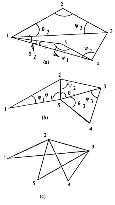
When there are more than three landmarks, there is no unique way of triangulation that characterizes the configuration of the landmarks. Some possible triangulations with five landmarks, prosthion (1), nasion (2), lambda (3), basion (4), and staphylion (5), on hominid skulls chosen for our study are indicated in Fig. 4.

Figure 4.

Different possible triangulations of landmarks.

All of the triangles in Fig. 4 a and b have a common vertex, 1 and 5, respectively, and in Fig. 4c, they have a common side: 2–3. In general, there may be some advantage in using Delaunay triangulation, which provides triangles close to the equilateral. In our case, the triangulation indicated in Fig. 4b corresponds to Delaunay triangulation. Because each triangle can be specified by two angles, there are altogether six independent angles describing the shape of an object. It may be noted that the triangulation in Fig. 4c is similar to Bookstein’s scheme of choosing a line joining any two landmarks and another line perpendicular to it as coordinate axes to specify the coordinates of the rest of the landmarks.

What triangulation should one choose for statistical analysis? There are two stages in statistical analysis in comparing populations for differences in shape. One is to establish by an appropriate test whether there are any shape differences. The other is to specify the nature of differences in shape. For the first object, any particular triangulation will do, provided that we can find an appropriate stochastic model for the corresponding angles. In practice one may choose two or more different triangulations to check the consistency of results. Once differences in shape are established, it may be necessary to consider all possible triangles formed by choosing all possible sets of three landmarks to specify the nature of differences in shape. First, we examine the differences in the shapes of hominid crania by types of apes (Pan troglodytes, Gorilla gorilla, and Pongo pygmaeus) and sex (male and female), by using the data collected by Paul O’Higgins and studied by O’Higgins and Dryden (8). We compare the results of two triangulations (Fig. 4 a and b) for consistency. At the next step, we examine the nature of the shape difference between the males of Pan and Pongo, the two apes found to be most dissimilar among the three types of apes.

The mean values for the angles as indicated in Fig. 4 a and b for two triangulations are given in Tables 4 and 5.

Table 4.

Mean values of angles—triangulation I

	Pan		Gorilla		Pongo
	Male (28)	Female (26)	Male (29)	Female (30)	Male (30)	Female (24)
θ1	0.0301	0.0365	0.0947	0.0406	0.1446	1.3070
θ2	0.2727	0.3018	0.2917	0.2910	0.3472	0.3644
θ3	0.5202	0.4929	0.4229	0.4850	0.2585	0.3332
ψ1	3.0752	3.0607	2.9249	3.0457	2.8417	2.8627
ψ2	2.3262	2.2674	2.1789	2.2715	2.0500	2.0980
ψ3	0.3429	0.3164	0.3094	0.3416	0.2079	0.2202

Table 5.

Mean values of angles—triangulation II

	Pan		Gorilla		Pongo
	Male (28)	Female (26)	Male (29)	Female (30)	Male (30)	Female (24)
θ1	1.3287	1.3072	1.2336	1.2815	1.3684	1.2324
θ2	1.3762	1.3763	1.2597	1.3273	0.9987	1.1428
θ3	0.4381	0.4921	0.4326	0.4601	0.4746	0.4914
ψ1	0.7924	0.7791	0.8088	0.8068	0.7503	0.8266
ψ2	1.2580	1.2771	1.3101	1.2617	1.6524	1.5056
ψ3	0.3783	0.4007	0.4086	0.3681	0.4617	0.4061

The square of the Mahalanobis distance between two populations with mean values μ₁, μ₂, and common covariance matrix Σ is defined by

which is estimated by

where x̄₁ and x̄₂ are the sample mean vectors and S is the pooled sum of squares and products matrix based on n degrees of freedom [see Rao (9)]. Hotelling’s T², which provides a test for the hypothesis μ₁ = μ₂, is

where n₁ and n₂ are sample sizes on which x̄₁ and x̄₂ are based. The above statistic has an F distribution on p and n − p + 1 degrees of freedom. In our problem, n = 167 − 6 = 161. The D² and T² values for testing differences between groups by sex and differences between sexes within each group are reported in Tables 6 and 7.

Table 6.

D² and T² values for differences between species by sex

Species	Males			Females
	D2	T2	p-value	D2	T2	p-value
Pan ∼ Gorilla
Triangulation I	10.37	23.85	<0.001	2.17	4.88	<0.001
Triangulation II	12.50	28.76	<0.001	5.84	13.13	<0.001
Gorilla ∼ Pongo
Triangulation I	28.57	68.03	<0.001	18.06	38.89	<0.001
Triangulation II	30.51	72.65	<0.001	19.84	42.72	<0.001
Pongo ∼ Pan
Triangulation I	43.11	100.84	<0.001	17.77	35.81	<0.001
Triangulation II	45.31	105.96	<0.001	20.56	41.45	<0.001

Table 7.

D² and T² values for differences between sexes within species

Species	Triangulation I			Triangulation II
	D2	T2	p-value	D2	T2	p-value
Pan	0.75	1.63	0.141	1.29	2.80	0.013
Gorilla	5.51	13.12	<0.001	5.90	14.04	<0.001
Pongo	9.04	19.46	<0.001	9.29	21.36	<0.001

All T² values have low p-values except for the difference between Pan males and females, showing significant differences in shape. Some interesting observations arising out of the study of T² and D² values are as follows. There are no inconsistencies in the conclusions based on the two triangulations of the landmarks. The D² values for comparing the males of different species are somewhat larger than the corresponding D² values for females, indicating that shapes of female crania of different apes are more similar than the shapes of the male crania of different apes. Among the hominids, Pan and Gorilla are closer in the shape of the crania, and Pongo is more distant.

3.2. Test for Sexual Dimorphism.

The difference in shape between male and female crania seems to be of different orders of magnitude, judged by the D² values, in the three species, indicating sexual dimorphism, which can be tested as follows. Let d_c, d_g, and d₀ be the vectors of differences in mean values of six angles between males and females in the Pan (chimpanzee), Gorilla, and Pongo (orangutan) samples. To d_c we attach a weight w_c = (28 × 26)/(28 + 26), where the numbers 28 and 26 are the sample sizes for Pan males and females. Similarly, we compute the weights w_g and w₀, for Gorilla and Pongo (orangutan) samples. Then, we compute what is called the sum of squares and products matrix between the species using the formula

where w = w_c + w_g + w₀ and

To this (6 × 6) matrix we attach q = 2 degrees of freedom. The pooled sum of squares and products matrix used in the computations of D² and T² values is the 6 × 6 matrix S, based on n = 161 degrees of freedom. We compute the Wilks Λ statistic to test for sexual dimorphism

The significance of Λ is assessed by using Rao’s transformation of Λ into F by the following computations:

F is approximately distributed as F on pq = 12 and ms = 312 degrees of freedom. The p-values for F = 7.3991 based on 12 and 312 degrees of freedom is small, indicating sexual dimorphism.

3.3 Canonical Coordinates for Graphical Representation.

Rao (10) developed the concept of canonical coordinates for representing the relative positions of the populations under study, which are characterized by a number of measurements (6 angles in the present problem), in a low-dimensional space. For this we consider the 6 × 6 matrix X of mean values with rows representing the variables (6 angles) and columns the populations (6 groups of hominids) and compute the “between sums of squares and products” matrix

where I₆ is a diagonal matrix with unities on the diagonal and J₆ is a 6 × 6 matrix with unity as all entries. Let W = n⁻¹S, where n is the degrees of freedom and S is the pooled sums of squares and products. Then we compute the eigenvalues and eigenvectors using the determinantal equation

where W^1/2 is the symmetric square root of W. If λ_i and l_i, i = 1, … , 6 are the eigenvalues and the corresponding eigenvectors, then the canonical coordinates in different dimensions (after translation to a suitable origin) are X′W^−1/2l_i, i = 1, … , 6, as given Table 8.

Table 8.

Canonical coordinates in the first three dimensions

Species	Dimension
	1	2	3
Pan males (c1)	0.256	1.461	1.526
Pan females (c2)	1.625	1.906	1.041
Gorilla males (g1)	1.863	−1.140	0.539
Gorilla females (g2)	0.800	0.749	0.779
Pongo males (o1)	6.763	0.658	1.646
Pongo females (o2)	3.695	2.093	0.0123

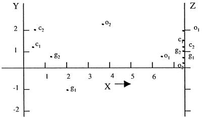
The eigenvalue λ_i represents the variance between populations in the ith dimension or variance as explained by the ith canonical coordinates. The values of λ_i and the percentage of variance explained by canonical coordinates are given in Table 9. It is seen that the first two canonical coordinates account for 99.7% of the variance and the first three canonical coordinates explain most of the variance due to six angles.

Table 9.

Percentage of variance explained

i	1	2	3	4	5	6
λi	0.9585	0.0384	0.0028	0.0002	0.0000	0.0000
%	95.90	99.70	99.98	100.00	—	—

The relative positions of the six populations under study are shown in Fig. 5, where the x and y axes represent the first two canonical coordinates and the third canonical coordinates are plotted on the vertical line to indicate any additional differences between groups in the third dimension. The relative positions of the groups are as inferred in Section 3.1 based on D² values and tests of significance.

Figure 5.

The configuration of the male and female apes in the dimensions of the first three canonical coordinates.

3.4. Interpretation of Differences Between Populations.

When overall differences in shape between populations are indicated by appropriate tests, it may be of interest to examine the nature of differences and to determine whether the differences are localized to some subconfigurations of the landmarks. We illustrate the method for such a study using the male Pan and Pongo apes.

We consider all possible sets of three out of five landmarks chosen for study. There are 10n such sets giving rise to 10 triangles, and we examine the difference between the two groups in the shape of each triangle. Table 10 gives the mean values of angles for each triangle for each of the two groups and the associated D² and T² values. Here the Hotelling’s T² test follows the F distribution with 2 and 55 degrees of freedom.

Table 10.

Mean angles, Mahalanobis’s D², and Hotelling’s T² for all possible triangles in the Pan and Pongo samples

Δ	Pan			Pongo			D2	T2	p-value
	ψ	θ	φ	ψ	θ	φ
123	0.520	0.343	2.280	0.258	0.208	2.676	26.252	186.705	<0.001
124	0.793	0.668	1.682	0.606	0.592	1.945	18.940	134.706	<0.001
125	0.792	1.329	1.022	0.750	1.368	1.024	0.624	4.438	0.016
134	0.272	2.326	0.544	0.347	2.050	0.746	7.699	54.757	<0.001
135	0.272	2.705	0.166	0.492	2.367	0.284	10.621	75.534	<0.001
145	0.030	3.075	0.037	0.146	2.842	0.156	8.890	63.227	<0.001
234	0.597	1.658	0.887	0.732	1.457	0.953	6.497	46.210	<0.001
235	1.258	1.376	0.508	1.652	0.999	0.492	25.954	184.588	<0.001
345	0.378	0.438	2.326	0.462	0.474	2.206	2.564	18.235	<0.001
245	0.660	1.814	0.668	0.921	1.473	0.749	19.332	137.492	<0.001

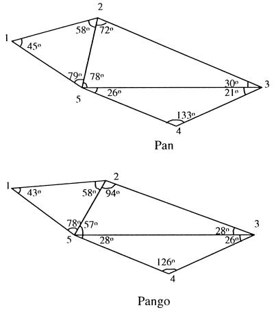
It is seen that the D² values for the triangles 125 and 345 are small, indicating that the relative positions of the landmarks 1, 2, and 5 and 3, 4, and 5 are nearly the same for Pan and Pongo. The major difference is in the relative positions of landmarks 2, 3, and 5, with 2 moving toward 3 and with the angle 235 remaining the same. The mean shapes of the crania of Pan and Pongo apes are shown in Fig. 6.

Figure 6.

Differences in shapes of Pan and Pongo.

This raises the question of whether the difference in the shape of triangle 235 has caused the difference in the shapes of other triangles or whether there are other factors also affecting the differences in the other triangles. To test this phenomenon, let us consider triangles 235, 123, and 234, which specify the configuration of the five landmarks. The D₂² value for triangle 235 (2 angles) is 25.954, as given in Table 10. The D₆² value for all of the triangles, 235, 123, and 234 (6 angles), is 37.688. The additional D² due to triangles 123 and 234 independently of the triangle 235 is D₆² − D₂² = 37.688 − 25.954 = 11.734, whereas the individual D² values due to these triangles are 26.252 and 6.497, respectively (as given in Table 10). Thus the differences is shapes of triangles 123 and 234 are largely explained by the difference in the shape of triangle 235.

The significance of D₆² − D₂² can, however, be tested by Rao’s U statistic [see Rao (9), p. 568]:

which as F on 4 and 51 degrees of freedom (using the values n₁ = 28, n₂ = 30) has a p-value of 0.002. The test indicates some additional differences due to triangles 123 and 234 to be explained, though smaller in magnitude.

What is the mean configuration of landmarks on an object? There are several definitions in the literature depending on the choice of shape measurements characterizing the configuration of landmarks on an object. We refer to a recent review paper by Molchanov (11) on this subject. We believe that the mean configuration has to be viewed in terms of the mean configurations of all possible triangles formed from different sets of three landmarks, as in Table 10. Further work is in progress.

4. Angular Measurements of Profile Between Landmarks

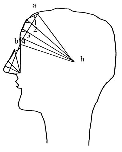
Although the angular data based on any particular triangulation of landmarks specify the configuration of landmarks, some further data may be generated to characterize the profile between landmarks if available, which may provide some additional information in problems of discrimination and identification. Let us consider the human facial profile (Fig. 7) and the triangle formed by the landmarks h, a, and b. We divide the angle ∠ahb, say h⁰, into k equal parts and draw lines at angles h⁰/k, h⁰/2k, . . . to the line ah. With k = 4, we have three lines, as shown in Fig. 7, which meet the profile between the landmarks a and b at three points. We now measure the four angles (1, 2, 3, 4), as shown in Fig. 7, which provide measurements on the shape of the profile. The process can be repeated with all the other basic triangles by choosing suitable values of k for each of the triangles. The angles of the basic triangles and the new angles generated by the process described above can be used in statistical analysis.

Figure 7.

Angular measurements of the human profile.

References

- 1.Rao C R, Suryawanshi S. Proc Natl Acad Sci USA. 1996;93:12132–12136. doi: 10.1073/pnas.93.22.12132. [DOI] [PMC free article] [PubMed] [Google Scholar]
- 2.Lele S. Math Geol. 1993;25:573–602. [Google Scholar]
- 3.Bookstein F L. Morphometric Tools for Landmark Data Geometry and Biology. Cambridge, U.K.: Cambridge Univ. Press; 1991. [Google Scholar]
- 4.Aitchison J. The Statistical Analysis of Compositional Data. Chapman and Hall; 1986. [Google Scholar]
- 5.Pukkila T M, Rao C R. Information Sci. 1988;45:379–389. [Google Scholar]
- 6.Mardia K V. Statistics of Directional Data. New York: Academic; 1972. [Google Scholar]
- 7.Rao, C. R. & Ali, H. (1998) Student, in press.
- 8.O’Higgins P, Dryden I L. J Hum Evol. 1993;24:183–205. [Google Scholar]
- 9.Rao C R. Linear Statistical Inference and Its Applications. New York: Wiley; 1973. [Google Scholar]
- 10.Rao C R. J R Stat Soc B. 1948;10:159–203. [Google Scholar]
- 11.Molchanov I S. Proc Int Stat Inst. 1997;1:119–122. [Google Scholar]