One- and two-body decomposable Poisson-Boltzmann methods for protein design calculations

Abstract

Successfully modeling electrostatic interactions is one of the key factors required for the computational design of proteins with desired physical, chemical, and biological properties. In this paper, we present formulations of the finite difference Poisson-Boltzmann (FDPB) model that are pairwise decomposable by side chain. These methods use reduced representations of the protein structure based on the backbone and one or two side chains in order to approximate the dielectric environment in and around the protein. For the desolvation of polar side chains, the two-body model has a 0.64 kcal/mol RMSD compared to FDPB calculations performed using the full representation of the protein structure. Screened Coulombic interaction energies between side chains are approximated with an RMSD of 0.13 kcal/mol. The methods presented here are compatible with the computational demands of protein design calculations and produce energies that are very similar to the results of traditional FDPB calculations.

Electrostatic interactions are often critical determinants of protein structure and function. In an earlier protein design study, an overly simplistic electrostatic model was found to incorporate destabilizing electrostatic interactions into the designed proteins (Marshall et al. 2002). Energies calculated using the finite difference Poisson-Boltzmann (FDPB) model (Gilson et al. 1987; Honig and Nicholls 1995; Rocchia et al. 2001), a more sophisticated model for describing the electrostatic potential in proteins, correlated more strongly with experimentally determined stability. However, FDPB calculations, as normally performed, are computationally too costly for most protein design calculations.

Computational protein design algorithms (Gordon et al. 1999; Street and Mayo 1999; Kraemer-Pecore et al. 2001; Mendes et al. 2002) have relied on simple, often empirical methods to model electrostatic interactions between charged and polar protein groups and the desolvation of polar and charged side chains. For example, the ORBIT (Optimization of Rotamers by Iterative Techniques) protein design force field uses Coulomb’s law with a distance-dependent dielectric and an explicit hydrogen-bond term to describe interactions between polar and charged groups and either a penalty for the burial of polar hydrogens or a penalty for the burial of polar surface area (Dahiyat and Mayo 1996; Gordon et al. 1999). Havranek and Harbury have developed a modified Tanford-Kirkwood model to describe electrostatic interactions and applied it to the design of homodimeric and heterodimeric coiled coils (Havranek and Harbury 1999, 2003). Baker and coworkers have used a volume-based solvent exclusion model to describe the desolvation of polar groups (Lazaridis and Karplus 1999), along with a distance-dependent dielectric model, in the successful design of a novel protein fold (Kuhlman et al. 2003). Recently, Hellinga and coworkers have empirically derived a large number of dielectric constants and interaction parameters to describe polar desolvation as well as charge–charge and charge–polar interactions between protein groups (Wisz and Hellinga 2003) and used these parameters to engineer catalytic function into a catalytically inert scaffold (Dwyer et al. 2004). Finally, Pokala and Handel (2004) have proposed a method for calculating Born radii in the context of protein design calculations.

Here, we describe a method for modeling electrostatic interactions in protein design calculations using a limited number of FDPB calculations performed with simplified surface representations. Typically, FDPB calculations require atomic coordinates for the protein backbone and all side chains in order to define the spatial regions that correspond to the low dielectric protein and high dielectric solvent. In protein design calculations, each possible rotameric sequence (a rotamer is a low energy amino acid side-chain conformation) will have a unique structure and require an independent FDPB calculation. Because the combinatorial complexity of design calculations is often astronomically large, it is not feasible to perform an independent calculation for each possible structure. Instead, we determine the electrostatic energy for each side chain or pair of side chains by performing FPDB calculations using simplified structures that include only the backbone and one or two side chains. The total energy is then obtained by summing the contribution of each side chain and side-chain pair.

Like the other electrostatic models that have been used for design, the simplified surface approach possesses the computational efficiency required for combinatorially complex protein design calculations. The method is two-body decomposable (meaning that each energy term depends on the identity and conformation of at most two amino acid side chains) and therefore compatible with deterministic search algorithms such as Dead End Elimination (DEE) (Desmet et al. 1992; Goldstein 1994; Gordon et al. 2003) that are often used for sequence selection. The two-body FDPB method described in this paper allows for calculation of both desolvation energies and electrostatic interactions between polar protein groups using a minimal number of free parameters. It explicitly captures the impact of sequence changes on the structure of the protein surface, which defines the boundary between the low dielectric protein and the high dielectric solvent. Finally, it efficiently produces energies that correlate well with standard FDPB methods, providing the accuracy demanded by protein design problems.

Strategies for incorporating FDPB methods into protein design calculations

In this study, we have used the FDPB solver from the computer program DelPhi (Rocchia et al. 2001) to calculate electrostatic energies for 24 proteins selected from a group of 500 high resolution protein X-ray structures compiled by Richardson and coworkers (Lovell et al. 2003). The results of these “exact” FDPB calculations were compared to the results of a tractable number of FDPB calculations performed using simplified surface representations that require knowledge of the identity and conformation of no more than two amino acid side chains at a time in order to assess the accuracy of the simplified surface approximation.

Polar protein groups can form favorable electrostatic interactions with the solvent; we refer to the resulting energies as electrostatic solvation energies. The difference between the electrostatic solvation energy of a polar group in the folded state versus the unfolded state is the desolvation energy. In design calculations, the backbone conformation is typically held fixed. As shown in Figure 1A ▶, the desolvation energy of the protein backbone can therefore be defined as the difference between the electrostatic solvation energy of the backbone in the presence of all of the protein’s side chains versus the electrostatic solvation energy of the isolated backbone (a reference state that remains constant in the design calculation). As shown in Figure 2A ▶, the desolvation energy of a side chain is defined as the difference between the electrostatic solvation energy of the side chain in the context of the folded protein versus the electrostatic solvation energy of the side chain and local backbone alone, where the local backbone is defined by the atoms CA(i − 1), C(i − 1), O(i − 1), N(i), H(i), CA(i), C(i), O(i), N(i + 1), H(i + 1), and CA(i + 1).

Figure 1.

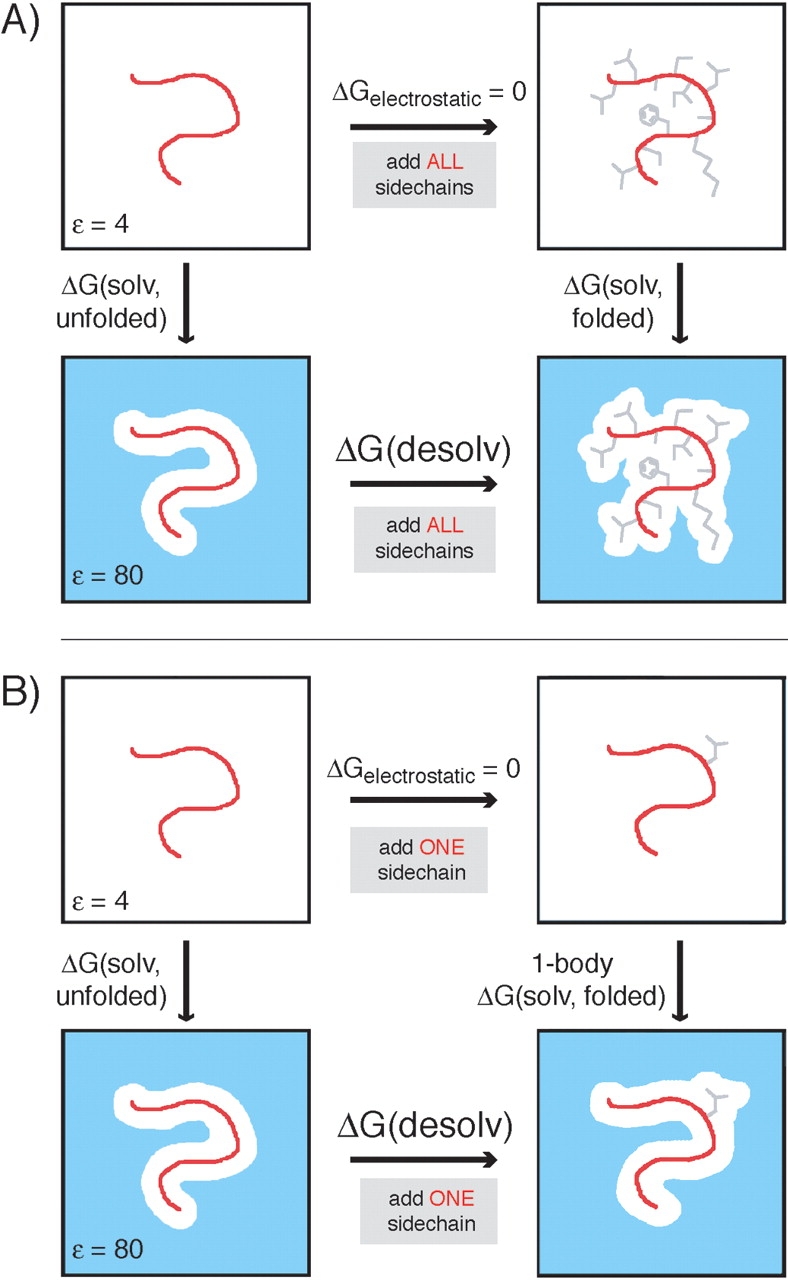
Free energy cycles used to calculate exact (A) vs. one-body (B) backbone desolvation energies (as shown in Equations 2 and 8, respectively). In each method, the electrostatic potential generated by the backbone is calculated. The key distinctions between the two methods are as follows: The exact calculation uses the protein backbone and all of the side chains in the protein to define the dielectric boundary, while in the one-body method, the dielectric boundary is defined by the backbone and a single side chain only. The total one-body desolvation is calculated by summing the desolvation by each side chain. The parameters used in each FDPB calculation are indicated as follows: the protein backbone, shown in red, was assigned partial atomic charges from the PARSE charge set; the side chains, shown in gray, were assigned partial atomic charges of 0; the areas drawn in white were assigned a dielectric constant of 4 (protein interior); and the blue areas were assigned a dielectric constant of 80 (water) and a salt concentration of 50 mM.

Figure 2.

Free energy cycles used to calculate exact side-chain desolvation energies (as shown in Equation 3) and side-chain/backbone screened Coulombic energies (A) (as shown in Equations 4 and 5) vs. one-body and two-body side-chain desolvation energies (B) (as shown in Equations 9 and 12, respectively) and side-chain/backbone screened Coulombic energies (C) (as shown in Equations 10 and 11, and 13 and 14, respectively). In each method, the electrostatic potential generated by side chain i is calculated. This potential is multiplied by the charges of side chain i to calculate the solvation energy of i and is multiplied by the charges in the backbone to determine the side-chain/backbone screening energy. The key distinctions between the exact, one-body, and two-body methods are as follows: The exact calculation uses the protein backbone and all of the side chains in the protein to define the dielectric boundary, and a single calculation is used to determine the folded-state solvation energy. In the one-body method, the dielectric boundary is defined by the backbone and a single side chain only. The one-body desolvation energy consists of the desolvation of side chain i by the backbone. In the two-body method, a one-body calculation is first performed as shown in parts B and C, and then the perturbation in the side-chain desolvation energy and the side-chain/backbone screened Coulombic energy that results from adding a second side chain, j, to the low dielectric protein region is determined. The perturbation due to each other side chain is added to the one-body energy to produce the two-body energy. The parameters used in each FDPB calculation are indicated as follows: side chain i, shown in red, was assigned partial atomic charges from the PARSE charge set; the rest of the protein, when shown in gray, was assigned partial atomic charges of 0; the protein backbone, when shown in green, was assigned partial atomic charges of 0 in the FDPB calculation, but its PARSE partial atomic charges were used to obtain screening energies; the areas drawn in white were assigned a dielectric constant of 4 (protein interior); and the blue areas were assigned a dielectric constant of 80 (water) and a salt concentration of 50 mM.

Electrostatic interactions between polar protein groups and the solvent also act to screen Coulombic interactions within a protein. The screening energy is generally opposite in sign and weaker in magnitude than the Coulombic energy for a given interaction. The procedures used to calculate side-chain/backbone and side-chain/side-chain screening energies are shown in Figures 2A ▶ and 3A ▶, respectively. In all cases, the screening energies and Coulombic energies are added to yield “screened Coulombic energies,” and the screened Coulombic energies predicted by the different electrostatic models are then compared. As solvation energies are strongly anticorrelated with Coulombic energies, comparison of screened Coulombic energies but not screening energies alone is appropriate for the validation of approximate electrostatic models (Scarsi and Caflisch 1999).

Figure 3.

Free energy cycles used to calculate exact (A) vs. two-body (B) side-chain/side-chain screened Coulombic energies (as shown in Equations 6 and 7, and 15 and 16, respectively). In each method, the electrostatic potential generated by side chain i is multiplied by the charges in side chain j to determine the screening energy between side chain i and side chain j. The key distinctions between the exact and two-body methods are as follows: The exact calculation uses the protein backbone and all of the side chains in the protein to define the dielectric boundary, while the two-body calculation uses the protein backbone and only two side chains to define the dielectric boundary. The parameters used in each FDPB calculation are indicated as follows: side chain i, shown in red, was assigned partial atomic charges from the PARSE charge set; the rest of the protein, when shown in gray, was assigned partial atomic charges of 0; side chain j, when shown in green, was assigned partial atomic charges of 0 in the FDPB calculation, but its PARSE partial atomic charges were used to obtain screening energies; the areas drawn in white were assigned a dielectric constant of 4 (protein interior); and the blue areas were assigned a dielectric constant of 80 (water) and a salt concentration of 50 mM.

For compatibility with the ORBIT protein design procedure, we have calculated backbone desolvation energies, side-chain desolvation energies, side-chain/backbone interaction energies, and side-chain/side-chain interaction energies separately. The total electrostatic energy of each rotameric state of a protein is then the sum of the backbone desolvation energy (ΔG^bb_desolv), the desolvation energy of each side chain i (ΔGⁱ_desolv), the screened Coulombic interaction between each side chain i and the backbone (ΔG^i/bb_screenedCoul), and the screened Coulombic interaction between each pair of side chains i and j (ΔG ^i/j_screenedCoul):

(1)

When calculating the “exact” FDPB energies, each of the above terms is calculated using all of the protein atoms to define the low dielectric protein region versus the high dielectric solvent region.

One-body FDPB decomposition

Several physical properties of proteins can be calculated using information derived from the protein surface. While protein surfaces cannot be perfectly represented using pairwise decomposable methods, earlier protein design studies have demonstrated that pairwise or sequence-independent approximations can yield satisfactory results for hydrophobic solvation and binary patterning, respectively (Street and Mayo 1998; Marshall and Mayo 2001). Similarly, it may be possible to obtain accurate estimates of the FDPB energies obtained using all the atomic coordinates to define the surface from FDPB energies obtained using simplified models for the protein surface that require knowledge of only one or two side-chain conformations at a time.

Since the protein backbone is fixed during design calculations, an approximate one-body (i.e., one side-chain rotamer) surface can be obtained using the atoms from the protein backbone and the side chain of interest only. It is necessary to include the side chain of interest when defining the protein surface to ensure that all protein charges are located in the low dielectric protein region rather than the high dielectric solvent region. The one-body backbone desolvation energy, which is an approximation of the desolvation of the backbone by each side chain, is calculated as the difference in solvation energy between the one-body folded state (which includes only the side chain of interest and the backbone) and the isolated backbone, as shown in Figure 1B ▶. The total backbone desolvation energy for each protein is approximated as the sum of the one-body backbone desolvation energies of each of its side chains. As is shown in Figure 2B ▶, one-body side-chain desolvation energies are calculated as the difference in solvation energy between the one-body folded state (which includes only the side chain of interest and the backbone) and the unfolded state (which includes side chain i and the local backbone). The one-body side-chain/backbone screened Coulombic energy of each side chain is calculated using the model in Figure 2C ▶.

To test the accuracy of the one-body decomposition, we calculated the backbone desolvation energies, side-chain desolvation energies, and side-chain/backbone screened Coulombic energies for the set of 24 proteins. Backbone desolvation energies can be calculated reasonably well by summing the desolvation induced by the presence of each side chain, as shown in Figure 4A ▶. Using the one-body decomposition, the backbone desolvation energy resulting from each side chain can be considered as a component of the side-chain/backbone energy of the side chain in design calculations. The extent to which backbone desolvation energy depends on protein sequence and side-chain conformations is not yet fully understood. Avbelj, Baldwin, and coworkers, however, have reported the importance of backbone desolvation in determining amino acid secondary structure propensities (Avbelj and Moult 1995; Avbelj and Fele 1998; Avbelj et al. 2000).

Figure 4.

Accuracy of the one-body method determined by comparing exact FDPB backbone desolvation energies vs. one-body backbone desolvation energies (A), exact FDPB side-chain desolvation energies vs. one-body side-chain desolvation energies (B), and exact FDPB side-chain/backbone screened Coulombic energies vs. one-body side-chain/backbone screened Coulombic energies (C).

The one-body approximation grossly underestimates the majority of the side-chain desolvation and side-chain/backbone screened Coulombic energies, as shown in Figure 4, B and C ▶, respectively. The one-body model neglects the contribution of the other side chains to the dielectric environment of the side chain of interest, resulting in an excessively solvated folded state. Deviations between the one-body and exact FDPB results are especially pronounced for large magnitude desolvation and screened Coulombic energies, which tend to occur in environments with a low effective dielectric.

Two-body FDPB decomposition

More accurate energies can be obtained using two-body methods (i.e., methods including two side-chain rotamers), in which the total side-chain desolvation or side-chain/backbone screened Coulombic energy for each side chain i is defined as the sum of its one-body energy and the two-body perturbation energies for each other side chain j. As shown in Figure 2, B and C ▶, the perturbation energy of each other side chain is defined as the difference between the two-body energy, which is calculated using the backbone and two side chains to define the dielectric boundary, and the one-body energy calculated previously.

Incorporating the effects of other side chains using the two-body perturbation method allows accurate calculation of electrostatic energies, as shown in Table 1 and Figure 5, A and B ▶. Five outlier points, representing five different amino acid types from four structures, were observed to have large errors in their two-body side-chain desolvation energies, as shown in Figure 5A ▶. These outliers likely arise from grid placement artifacts, a source of error in FDPB calculations that has been described previously (Gilson et al. 1987). Accurate two-body desolvation energies can be obtained for these five points by slightly altering the position of the molecule relative to the grid (data not shown).

Table 1.

Accuracy of the electrostatic models

	RMSD (kcal/mol)	R
A. Backbone desolvation energy
Exact FDPB	—	—
One-body	3.96	0.997
B. Side-chain desolvation energy
Exact FDPB	—	—
One-body	1.93	0.718
Two-body,a all pairs	0.64	0.962
Two-body,a pairs <6 Å	0.67	0.968
Two-body,a pairs <4 Å	0.82	0.952
C. Side-chain/backbone screened Coulombic energy
Exact FDPB	—	—
One-body	0.90	0.957
Two-body, all pairs	0.36	0.987
Two-body, pairs <6 Å	0.41	0.984
Two-body, pairs <4 Å	0.51	0.979
D. Side-chain/side-chain screened Coulombic energy
Exact FDPB	—	—
Two-body, all pairs	0.13	0.948

Statistics were obtained using all data points, including outliers, and without application of α, the scaling parameter for two-body side-chain desolvation.

Figure 5.

Accuracy of the two-body method determined by comparing exact FDPB side-chain desolvation energies vs. two-body side-chain desolvation energies with outlier points represented by open circles (A), exact FDPB side-chain/backbone screened Coulombic energies vs. two-body side-chain/backbone screened Coulombic energies (B), and exact FDPB side-chain/side-chain screened Coulombic energies vs. two-body side-chain/side-chain screened Coulombic energies (C).

The two-body approximation systematically underestimates the magnitude of the side-chain desolvation energy. The systematic error in the two-body desolvation energy was minimized by linearly scaling the two-body perturbation energy. The set of 24 structures was divided into two sets of 12 structures, and a scaling parameter, α, was derived by a linear least-squares fit for each set (with the five outlier points removed). The robustness of the scaling parameter was tested by cross-validation, as shown in Table 2, and sensitivity analysis, as shown in Figure 6A ▶. The error in the two-body side-chain desolvation is reasonably insensitive to α around the optimal α value, and both sets have similar dependence on α, suggesting that this scaling parameter should be used in routine calculations.

Table 2.

Cross-validation of α, the scaling parameter for two-body side-chain desolvation

	RMSD (kcal/mol)	R
Structure set 1
α = 1	0.56	0.967
α = 1.26a	0.43	0.972
α = 1.30b	0.43	0.973
Structure set 2
α = 1	0.68	0.971
α = 1.26a	0.50	0.974
α = 1.30b	0.50	0.974

^a The optimal value of α determined using structure set 1.

^b The optimal value of α determined using structure set 2.

Figure 6.

Sensitivity of error in two-body energies due to changes in α, the scaling parameter for two-body side-chain desolvation energies (A); the distance-dependent dielectric for pairs separated by >6.0 Å (B); and the distance-dependent dielectric for pairs separated by >4.0 Å (C). In all cases, filled symbols refer to protein structure set 1, open symbols refer to protein structure set 2, circles indicate RMSD, and triangles indicate the correlation coefficient R.

In the one-body FDPB method, we calculated side-chain and backbone desolvation energies and side-chain/backbone screening energies, but not side-chain/side-chain screening energies. Simply multiplying the one-body potential generated by side chain i by the partial atomic charges of side chain j is not very accurate (data not shown), especially for charged atoms located at or beyond the dielectric boundary defined by side chain i and the protein backbone. Side-chain/side-chain screened Coulombic energies were calculated using a two-body decomposable method that uses only the backbone and two side chains of interest to define the dielectric boundary, as shown in Figure 3B ▶. Although the two-body model systematically overscreens the Coulombic interactions, the accuracy obtained using a two-body FDPB decomposition is quite good, as shown in Table 1 and Figure 5C ▶. The two-body approximation is probably less accurate for certain large interaction energies owing to increased sensitivity to the shape of the dielectric boundary in regions of large electrostatic potential.

Analysis of the side-chain desolvation and side-chain/backbone screened Coulombic energies indicates that, in most cases, the perturbation caused by a second side chain is negligible. The small fraction of two-body perturbations that contribute significantly to the desolvation or side-chain/backbone energies involve pairs of residues that are close in space. Furthermore, side-chain/side-chain interaction energies for residues that are not close in space are typically small in magnitude and may be approximated using a simpler electrostatic model. We performed additional calculations in which two-body perturbations were calculated only for pairs that separated by <6 Å or 4 Å. As shown in Table 1, we observe a slight decrease in accuracy as the distance cutoff is decreased from infinity to 6 Å to 4 Å. This arises from an increased underestimation of the side-chain desolvation energies and side-chain/backbone screened Coulombic energies, as well as increased inaccuracy in defining the dielectric environment, as fewer pairs are included.

When calculating screened Coulombic energies, the interaction of side-chain pairs separated by more than a distance cutoff of 6 Å or 4 Å was approximated by a distance-dependent Coulombic model, and the two-body FDPB model was applied only to pairs that are close in space. The two sets of protein structures used for the α parameterization were used to derive the optimal distance-dependent dielectric values for pairs separated by distances greater than the cutoff. The dielectrics derived for each set are similar, and the errors in the two-body approximation with the cutoffs are comparable to the error in the full two-body calculation including all pairs, as shown in Table 3. The sensitivity of the error and correlation with the exact FDPB energies to the dielectric value is shown in Figure 6, B and C ▶.

Table 3.

Cross-validation of distance-dependent dielectrics for limited pair two-body side-chain/side-chain screened Coulombic interactions

	RMSDa (kcal/mol)	Ra
Structure set 1
All pairs	0.10	0.968
Pairs >6 Å, ɛ = 5.11rb	0.10	0.960
Pairs >6 Å, ɛ = 4.75rc	0.10	0.957
Pairs >4 Å, ɛ = 5.90rd	0.10	0.955
Pairs >4 Å, ɛ = 5.21re	0.10	0.947
Structure set 2
All pairs	0.16	0.934
Pairs >6 Å, ɛ = 5.11rb	0.16	0.926
Pairs >6 Å, ɛ = 4.75rc	0.16	0.923
Pairs >4 Å, ɛ = 5.90rd	0.16	0.924
Pairs >4 Å, ɛ = 5.21re	0.16	0.917

^a RMSD and R values are for all pairs in each structure set.

^b The optimal distance-dependent dielectric for pairs separated by > 6 Å in structure set 1.

^c The optimal distance-dependent dielectric for pairs separated by > 6 Å in structure set 2.

^d The optimal distance-dependent dielectric for pairs separated by > 4 Å in structure set 1.

^e The optimal distance-dependent dielectric for pairs separated by > 4 Å in structure set 2.

Considering only a limited subset of pairs significantly reduces the total calculation time, which is crucial since the number of pairs in a design calculation is often large. For instance, the reported surface design calculation for engrailed homeodomain considers 15,000,000 rotamer pairs (Marshall et al. 2002). The FDPB calculation for this number of pairs would require ~3 wk of CPU time on a cluster of 128 IBM PowerPC 970 processors running at 1.6 GHz. The time required to complete the two-body calculation can be reduced to <1 d of CPU time by applying a distance cutoff of 4.0 Å.

It has been shown that, for a series of designed homeodomain variants, there is a correlation between experimental stability and exact FDPB electrostatic energies plus ORBIT van der Waals energies (Marshall et al. 2002). In order to assess the predictive power of the two-body method presented here, we have compared the two-body FDPB energies to these experimental results. For each variant, the sum of all two-body side-chain/backbone and side-chain/side-chain screened Coulombic energies and the sum of all two-body side-chain desolvation energies were added to the ORBIT van der Waals energies. As shown in Figure 7 ▶, the two-body FDPB energies are able to predict, with accuracy close to that of the exact FDPB calculations, trends in experimental stabilities of six of the seven variants tested, including the wild-type protein and NC3-Ncap, the most stable variant.

Figure 7.

Energy predicted using the sum of the FDPB side-chain desolvation energy, FDPB side-chain/backbone screened Coulombic energy, FDPB side-chain/side-chain screened Coulombic energy, and ORBIT van der Waals energy vs. the experimentally determined stability of each ho-meodomain variant. The energies obtained using the two-body FDPB approximation are shown as filled circles, and the energies obtained using the exact FDPB model are shown as open circles.

Additional considerations

Thus far, we have developed and tested new electrostatic models for protein design calculations by maximizing the agreement between the approximate desolvation and screened Coulombic energies with the exact FDPB energies. While even “exact” FDPB energies are an approximation of the true electrostatic energy of the system, it is probable that, in the context of design calculations, the accuracy of the structural model will be a greater source of error than the limitations of the underlying FDPB model. To maximize computational efficiency, most protein design methods use a fixed backbone, discrete side-chain rotamers, and a very simple model of the unfolded state. As a result, certain errors in electrostatic energies can be observed in design calculations. For example, the energetic benefit of surface salt bridges is overestimated if the entropic cost of locking flexible side chains into a single conformation is not considered. Similarly, the folded-state stability conferred by interactions that are populated in the unfolded state, such as i, i ± 2 side-chain/backbone interactions, is overestimated if the unfolded state is modeled as the side chain and local backbone only.

Based on a single study of electrostatics in designed proteins (Marshall et al. 2002), either exact or two-body FDPB energies (with large magnitude side-chain/side-chain inter-actions truncated) are sufficiently accurate to provide a reasonable correlation with experimentally determined stability, as shown in Figure 7 ▶. Additional experimental studies will be required to assess the performance of the two-body decomposable model in the design of proteins with specific catalytic or binding properties. In cases where accurate modeling of electrostatics is especially critical, more sophisticated structural models, such as the flexible rotamer model (Mendes et al. 1999) and explicit modeling of alternate backbone conformations (Kuhlman et al. 2003), may prove useful.

Conclusions

Accurate electrostatic models, including the FDPB model, require knowledge of the full tertiary structure of the protein. As a result, these models cannot be applied directly to protein design calculations, which often consider >10⁵⁰ possible protein structures. While it is not possible to explicitly calculate electrostatic energies in each structural environment, it is also not prudent to neglect changes in the shape of a protein’s surface that result from modifying the protein sequence.

We have found that it is possible to obtain accurate electrostatic energies using simplified surface models that depend on the identity and conformation of the protein backbone and only one or two side chains at a time. The success of the two-body FDPB method suggests that it is critical to define the surface accurately in the immediate vicinity of the partial charges that are “generating” and “feeling” the electrostatic potential in each calculation. The results also suggest that it is important to account for desolvation and screening due to other nearby side chains, but that the effects of each other side chain are fairly independent and can be captured pairwise. Finally, we have found that the effects of sequence-dependent variation in the dielectric boundary can be neglected if the perturbations are reasonably far removed from the partial charges that are “generating” or “feeling” the electrostatic potential in a given calculation.

Efficient and accurate electrostatic models are also critical for protein folding and docking calculations. The simplified surface methods discussed here could be used to explore different side-chain orientations given a fixed-backbone conformation. Similarly, derivatives of a small molecule scaffold, such as those generated by combinatorial chemistry methods, could be modeled. However, folding and docking calculations typically sample a large number of backbone conformations or relative molecular orientations. Since each backbone conformation would require an independent set of one- or two-body FDPB calculations, the computational demands of folding and docking calculations would be far greater than those for design.

The stability of designed proteins has already been demonstrated to be sensitive to the quality of the electrostatic model used in the design calculations. It is likely that electrostatic interactions are at least as important in determining the functional properties of proteins, including binding and catalysis. As a result, the development and testing of accurate electrostatic models are likely to significantly aid in the design of proteins with desired physical, chemical, and biological properties.

Materials and methods

Test set of proteins

All calculations were performed using proteins selected from a group of 500 high resolution protein X-ray structures, including computationally optimized hydrogen atom locations, compiled by Richardson and coworkers (Lovell et al. 2003) (http://kinemage.biochem.duke.edu/databases/top500.php). Structural coordinates were derived from PDB entries 1IGD, 1MSI, 1KP6, 1OPD, 1FNA, 1MOL, 2ACY, 1ERV, 1DHN, 1WHI, 3CHY, 1ELK, 2RN2, 1HKA, 3LZM, 1AMM, 1XNB, 153L, 1BK7, 2PTH, 1THV, 1BS9, 1AGJ, and 2BAA, corresponding to the β1 domain of Streptococcal protein G, type III antifreeze protein, the α subunit of killer toxin KP6, the S46A mutant of Escherichia coli phosphotransferase, fibronectin cell-adhesion module type III, monellin, bovine acyl-phosphatase, the C73S mutant of human thioredoxin, 7,8-dihydroneopterin aldolase, the L14 ribosomal protein, CheY, the VHS domain of TOM1, ribonuclease H, pyrophosphokinase, T4 lysozyme, γ-B-crystallin, xylanase, goose lysozyme, ribonuclease MC1, peptidyl-tRNA hydrolase, thaumatin, acetylxylan esterase, epidermolytic toxin A from Streptococcus aureus, and endochitinase, respectively. Only the “A” chain was used for monellin, the VHS domain of TOM1, and epidermolytic toxin A.

Exact FDPB calculations

Finite difference solutions to the linearized Poisson-Boltzmann equation were obtained using the FDPB solver from the computer program DelPhi (Rocchia et al. 2001) with a grid spacing of 2.0 grids/Å⁻¹, an interior dielectric of 4.0, an exterior dielectric of 80.0, a salt concentration of 0.050 M, and a probe radius of 1.4 Å. The grid size was selected for each protein so that its backbone atoms fill 70% of the grid. The coordinates of each protein were mapped onto the grid in exactly the same way in all of the calculations to minimize errors due to changing grid placement. The PARSE parameter set charges and atomic radii (Sitkoff et al. 1994) were used in all FDPB calculations. Proline residues and cysteine residues in disulfide bonds were considered part of the backbone in all calculations. All Arg and Lys residues were modeled with a +1 net charge and all Asp and Glu residues were modeled with a −1 charge. All FDPB energies were converted to units of kilocalories per mol using the relation kT = 0.593 kcal/mol at 25°C.

In the FDPB model, electrostatic solvation energies are obtained by multiplying the appropriate atomic charges, q, by the reaction field potential, φ, at the location of each charge. In the following equations, the reaction field potential, φ, is labeled with a superscript that indicates which atoms were used to define the dielectric boundary and with a subscript that indicates which atoms were assigned nonzero partial atomic charges when calculating the reaction field potential. The entire protein is referred to as “all,” the protein backbone is referred to as “bb,” individual protein side chains are referred to as “i” or “j,” and a side chain with its local backbone is referred to as “ib.” A factor of ½ appears in the desolvation energy equations to account for the work of solvent polarization in response to the charges on side chain i.

The exact desolvation energy of the backbone (“bb”), shown in Figure 1A ▶, is defined as the difference between the electrostatic solvation energy of the backbone in the presence of all the protein side chains and the electrostatic solvation energy of the backbone alone:

(2)

where each t is a backbone atom, q_t is the partial atomic charge of backbone atom t, φ_bb^all is the reaction field potential at t generated by the set of partial atomic charges on the backbone when all of the protein atoms are used to define the dielectric boundary, and φ_bb^bb is the reaction field potential at t generated by the set partial atomic charges on the backbone when the backbone atoms only are used to define the dielectric boundary.

The exact desolvation energy of a side chain i, shown in Figure 2A ▶, is defined as the difference between the electrostatic solvation energy of the side chain in the folded state versus the unfolded state:

(3)

where each u is an atom in side chain i, q_u is the partial atomic charge of side-chain atom u, φ_i^all is the reaction field potential at u generated by the set of partial atomic charges on side chain i when all of the protein atoms are used to define the dielectric boundary, and φ_i^ib is the reaction field potential at u generated by the set of partial atomic charges on side chain i when the atoms on side chain i and its local backbone are used to define the dielectric boundary. The molecular surface for the side-chain unfolded-state model was generated using the side chain and local backbone and was mapped to the grid exactly as in the folded-state calculations. The local backbone was defined to include the following atoms: CA(i − 1), C(i − 1), O(i − 1), N(i), H(i), CA(i), C(i), O(i), N(i + 1), H(i + 1), and CA(i + 1).

Exact folded-state side-chain/backbone screening energies, shown in Figure 2A ▶, were obtained using the following equation:

(4)

where i is the side chain of interest, each t is an atom in the backbone, q_t is the partial atomic charge of atom t, and φ _i^all is the reaction field potential at t generated by the set of partial atomic charges on side chain i when all of the protein atoms are used to define the dielectric boundary. The screening energies were then added to the Coulombic energies to obtain screened Coulombic energies:

(5)

where the Coulombic energy is calculated using Coulomb’s law with a dielectric constant equal to the dielectric of the protein interior.

Exact side-chain/side-chain interactions, shown in Figure 3A ▶, were obtained using a similar method:

(6)

where i and j are the side chains of interest, each v is an atom in side chain j, q_v is the partial atomic charge of atom v, and φ _i^all is the reaction field potential at v generated by the set of partial atomic charges on side chain i when all of the protein atoms are used to define the dielectric boundary. The screening energies were then added to the Coulombic energies to obtain screened Coulombic energies:

(7)

Side-chain/backbone and side-chain/side-chain interaction energies are assumed to be zero in the unfolded state.

One-body FDPB calculations

One-body FDPB energies were calculated for backbone desolvation energies, side-chain desolvation energies, and side-chain/backbone screened Coulombic energies. For each side chain in the test set, two FDPB calculations are carried out: one with nonzero partial atomic charges assigned to the side chain and one with nonzero partial atomic charges assigned to the backbone. Folded-state solvation energies for the protein backbone were calculated as in the exact FDPB calculations, except that side chains other than the side chain of interest were not included:

(8)

where each t is a backbone atom, q_t is the partial atomic charge of backbone atom t, φ_bb^i,bb is the reaction field potential at t generated by the set of partial atomic charges on the backbone when side chain i and the backbone atoms only are used to define the dielectric boundary, and φ_bb^bb is the reaction field potential at t generated by the set of partial atomic charges on the backbone when the backbone atoms only are used to define the dielectric boundary, as shown in Figure 1B ▶. The total backbone desolvation energy for each protein is approximated by the sum of the one-body backbone desolvation energies, given by Equation 8, for each of its side chains.

Side-chain desolvation energies were calculated as in the exact FDPB calculations, except only the side chain of interest and the backbone were used to construct the folded-state dielectric boundary:

(9)

where i is the side chain of interest, each u is an atom in side chain i, q_u is the partial atomic charge of atom u, φ_i^i,bb is the reaction field potential at u generated by the set of partial atomic charges on side chain i when side chain i and the backbone atoms only are used to define the dielectric boundary, and φ_i^ib is the reaction field potential at u generated by the set of partial atomic charges on side chain i when the atoms in side chain i and its local backbone are used to define the dielectric boundary, as shown in Figure 2B ▶.

Similarly, side-chain/backbone screened Coulombic energies were calculated as in the exact FDPB calculations, except only the side chain of interest and the backbone were used to construct the dielectric boundary:

(10)

where i is the side chain of interest, each t is a backbone atom, q_t is the partial atomic charge of atom t, and φ_i^i,bb is the reaction field potential at t generated by the set of partial atomic charges on side chain i when side chain i and the backbone atoms only are used to define the dielectric boundary, as shown in Figure 2C ▶. The screening energies were then added to the Coulombic energies to obtain screened Coulombic energies

(11)

where the Coulombic energy is calculated using Coulomb’s law with a dielectric constant equal to the dielectric of the protein interior.

Two-body FDPB calculations

Two-body FDPB side-chain desolvation energies, side-chain/backbone screened Coulombic energies, and side-chain/side-chain screened Coulombic energies were calculated as follows. First, the one-body energies were calculated as described above. Next, two-body perturbation energies were calculated using the atoms in the backbone, bb, the side chain of interest, i, and one “perturbing” side chain, j, to define the dielectric boundary. Two-body perturbation energies were calculated using each residue other than the side chain of interest as the perturbing residue. Total energies were calculated by adding the one-body energy to the sum of the two-body perturbation energies. For each pair of side chains, two FDPB calculations are carried out, one with nonzero partial atomic charges assigned to each side chain.

Two-body side-chain desolvation energies were calculated as the sum of a one-body energy and two-body perturbation energies:

(12)

where i is the side chain of interest, each u is an atom in side chain i, q_u is the partial atomic charge of u, and φ_i^i,j,bb is the reaction field potential at u generated by the set of partial atomic charges on side chain i when the backbone and side chains i and j are used to define the dielectric boundary, as shown in Figure 2B ▶.

In order to improve the accuracy of the two-body side-chain desolvation energy, a scaling parameter, α, was multiplied by the term in Equation 12 that sums over side chains j. This parameter was fit using two distinct sets of structures. Structure set 1 contained 1IGD, 1KP6, 1FNA, 2ACY, 1DHN, 3CHY, 2RN2, 3LZM, 1XNB, 1BK7, 1THV, and 1AGJ. Structure set 2 contained 1MSI, 1OPD, 1MOL, 1ERV, 1WHI, 1ELK, 1HKA, 1AMM, 153L, 2PTH, 1BS9, and 2BAA. Optimum values of α were determined for each set by linear least-squares fit, and a sensitivity analysis was performed by testing values of α between 1.0 and 2.0 at intervals of 0.05.

Two-body side-chain/backbone screened Coulombic energies were calculated as the sum of a one-body energy and two-body perturbation energies:

(13)

where i is the side chain of interest, each t is a backbone atom, q_t is the partial atomic charge of t, and φ_i^i,j,bb is the reaction field potential at t generated by the set of partial atomic charges on side chain i when the backbone and side chains i and j are used to define the dielectric boundary, as shown in Figure 2C ▶. The screening energies were then added to the Coulombic energies to obtain screened Coulombic energies:

(14)

where the Coulombic energy is calculated using Coulomb’s law with a dielectric constant equal to the dielectric of the protein interior.

Two-body side-chain/side-chain calculations were calculated using the same method that was used to calculate the exact side-chain/side-chain screening energies, except that the dielectric boundary is defined using only the backbone and the two side chains of interest:

(15)

where i and j are the two side chains of interest, each v is an atom in side chain j, q_v is the partial atomic charge of atom v, and φ_i^i,j,bb is the reaction field potential at v generated by the set of partial atomic charges on side chain i when the backbone and side chains i and j are used to define the dielectric boundary, as shown in Figure 3B ▶. The screening energies were then added to the Coulombic energies to obtain screened Coulombic energies:

(16)

where the Coulombic energy is calculated using Coulomb’s law with a dielectric constant equal to the dielectric of the protein interior.

For the two-body side-chain desolvation and side-chain/backbone screened Coulombic energy calculations using only pairs that are close in space, the distance between side chains i and j was defined as the minimum distance between any atom with nonzero partial atomic charge on side chain i and any atom on side chain j. For two-body side-chain/side-chain screened Coulombic energy calculations using only pairs that are close in space, the distance between side chains i and j was defined as the minimum distance between any atom with nonzero partial atomic charge on side chain i and any atom with nonzero partial atomic charge on side chain j. In side-chain/side-chain calculations, Coulomb’s law was used to calculate the energy of pairs that were farther apart than the cutoff distance. For cutoff distances of both 6.0 Å and 4.0 Å, optimal distance-dependent dielectric values were derived by linear least squares to maximize agreement with the exact FDPB side-chain/side-chain screened Coulombic energies. These dielectric values were tested by cross-validation, and the sensitivity of the error in the two-body approximation with a cutoff was tested by varying the dielectric values.

Two-body energies were calculated for a series of homeodomain variants reported by Marshall et al. (2002). For each variant, FDPB two-body side-chain desolvation energies, two-body side-chain/backbone screened Coulombic energies, and two-body side-chain/side-chain screened Coulombic energies were added to the total ORBIT van der Waals energy. A threshold of ±0.90 kcal/mol was applied to the side-chain/backbone and side-chain/side-chain screened Coulombic energies. FDPB calculations were run using parameters described previously (Marshall et al. 2002).

Electronic supplemental material

Supplemental Figure 1 ▶ outlines how the methods described here can be implemented in a protein design calculation, including pseudocode for the one- and two-body FDPB calculations.

Article published online ahead of print. Article and publication date are at http://www.proteinscience.org/cgi/doi/10.1110/ps.041259105.

References

- Avbelj, F. and Fele, L. 1998. Role of main-chain electrostatics, hydrophobic effect and side-chain conformational entropy in determining the secondary structure of proteins. J. Mol. Biol. 279 665–684. [DOI] [PubMed] [Google Scholar]
- Avbelj, F. and Moult, J. 1995. Role of electrostatic screening in determining protein main-chain conformational preferences. Biochemistry 34 755–764. [DOI] [PubMed] [Google Scholar]
- Avbelj, F., Luo, P.Z., and Baldwin, R.L. 2000. Energetics of the interaction between water and the helical peptide group and its role in determining helix propensities. Proc. Natl. Acad. Sci. 97 10786–10791. [DOI] [PMC free article] [PubMed] [Google Scholar]
- Dahiyat, B.I. and Mayo, S.L. 1996. Protein design automation. Protein Sci. 5 895–903. [DOI] [PMC free article] [PubMed] [Google Scholar]
- Desmet, J., De Maeyer, M., Hazes, B., and Lasters, I. 1992. The dead-end elimination theorem and its use in protein side-chain positioning. Nature 356 539–542. [DOI] [PubMed] [Google Scholar]
- Dwyer, M.A., Looger, L.L., and Hellinga, H.W. 2004. Computational design of a biologically active enzyme. Science 304 1967–1971. [DOI] [PubMed] [Google Scholar]
- Gilson, M.K., Sharp, K., and Honig, B. 1987. Calculating the electrostatic potential of molecules in solution: Method and error assessment. J. Comput. Chem. 9 327–335. [Google Scholar]
- Goldstein, R.F. 1994. Efficient rotamer elimination applied to protein side-chains and related spin-glasses. Biophys. J. 66 1335–1340. [DOI] [PMC free article] [PubMed] [Google Scholar]
- Gordon, D.B., Marshall, S.A., and Mayo, S.L. 1999. Energy functions for protein design. Curr. Opin. Struct. Biol. 9 509–513. [DOI] [PubMed] [Google Scholar]
- Gordon, D.B., Hom, G.K., Mayo, S.L., and Pierce, N.A. 2003. Exact rotamer optimization for protein design. J. Comput. Chem. 24 232–243. [DOI] [PubMed] [Google Scholar]
- Havranek, J.J. and Harbury, P.B. 1999. Tanford-Kirkwood electrostatics for protein modeling. Proc. Natl. Acad. Sci. 96 11145–11150. [DOI] [PMC free article] [PubMed] [Google Scholar]
- ———. 2003. Automated design of specificity in molecular recognition. Nat. Struct. Biol. 10 45–52. [DOI] [PubMed] [Google Scholar]
- Honig, B. and Nicholls, A. 1995. Classical electrostatics in biology and chemistry. Science 268 1144–1149. [DOI] [PubMed] [Google Scholar]
- Kraemer-Pecore, C.M., Wollacott, A.M., and Desjarlais, J.R. 2001. Computational protein design. Curr. Opin. Chem. Biol. 5 690–695. [DOI] [PubMed] [Google Scholar]
- Kuhlman, B., Dantas, G., Ireton, G.C., Varani, G., Stoddard, B.L., and Baker, D. 2003. Design of a novel globular protein fold with atomic-level accuracy. Science 302 1364–1368. [DOI] [PubMed] [Google Scholar]
- Lazaridis, T. and Karplus, M. 1999. Effective energy function for proteins in solution. Proteins 35 133–152. [DOI] [PubMed] [Google Scholar]
- Lovell, S.C., Davis, I.W., Arendall III, W.B., de Bakker, P.I.W., Word, J.M., Prisant, M.G., Richardson, J.S., and Richardson, D.C. 2003. Structure validation by Cα geometry:φ , ψ, and Cβ deviation. Proteins 50 437–450. [DOI] [PubMed] [Google Scholar]
- Marshall, S.A. and Mayo, S.L. 2001. Achieving stability and conformational specificity in designed proteins via binary patterning. J. Mol. Biol. 305 619–631. [DOI] [PubMed] [Google Scholar]
- Marshall, S.A., Morgan, C.S., and Mayo, S.L. 2002. Electrostatics significantly affect the stability of designed homeodomain variants. J. Mol. Biol. 316 189–199. [DOI] [PubMed] [Google Scholar]
- Mendes, J., Baptista, A.M., Carrondo, M.A., and Soares, C.M. 1999. Improved modeling of side-chains in proteins with rotamer-based methods: A flexible rotamer model. Proteins 37 530–543. [DOI] [PubMed] [Google Scholar]
- Mendes, J., Guerois, R., and Serrano, L. 2002. Energy estimation in protein design. Curr. Opin. Struct. Biol. 12 441–446. [DOI] [PubMed] [Google Scholar]
- Pokala, N. and Handel, T.M. 2004. Energy functions for protein design I: Efficient and accurate continuum electrostatics and solvation. Protein Sci. 13 925–936. [DOI] [PMC free article] [PubMed] [Google Scholar]
- Rocchia, W., Alexov, E., and Honig, B. 2001. Extending the applicability of the nonlinear Poisson-Boltzmann equation: Multiple dielectric constants and multivalent ions. J. Phys. Chem. B 105 6507–6514. [Google Scholar]
- Scarsi, M. and Caflisch, A. 1999. Comment on the validation of continuum electrostatics models. J. Comput. Chem. 20 1533–1536. [Google Scholar]
- Sitkoff, D., Sharp, K., and Honig, B. 1994. Accurate calculation of hydration free energies using macroscopic solvent models. J. Phys. Chem. 98 1978–1988. [Google Scholar]
- Street, A.G. and Mayo, S.L. 1998. Pairwise calculation of protein solvent-accessible surface areas. Fold. Des. 3 253–258. [DOI] [PubMed] [Google Scholar]
- ———. 1999. Computational protein design. Struct. Fold. Des. 7 R105–R109. [DOI] [PubMed] [Google Scholar]
- Wisz, M.S. and Hellinga, H.W. 2003. An empirical model for electrostatic interactions in proteins incorporating multiple geometry-dependent dielectric constants. Proteins 51 360–377. [DOI] [PubMed] [Google Scholar]