Protein flexibility prediction by an all-atom mean-field statistical theory

Abstract

We extended a mean-field model to proteins with all atomic detail. The all-atom mean-field model was used to calculate the dynamic and thermodynamic properties of a three-helix bundle fragment of Staphylococcal protein A (Protein Data Bank [PDB] ID 1BDD) and α-spectrin SH3 domain protein (PDB ID 1SHG). We show that a model with all-atomic detail provides a significantly more accurate prediction of flexibility of residues in proteins than does a coarse-grained residue-level model. The accuracy of flexibility prediction is further confirmed by application of the method to 18 additional proteins with the largest size of 224 residues.

Dynamics of proteins plays an important role in function of proteins (Brooks et al. 1988). The ideal method to predict protein flexibility is to perform molecular dynamics simulation of proteins in aqueous solution with an accurate physical-based energy function (Brooks et al. 1983). The simulation, however, often requires long computational time. Thus, it is of interest to develop a simple efficient method to predict protein flexibility.

Several methods have been developed for an efficient flexibility prediction. The efficient prediction is accomplished by simplification of the model for proteins, the atomic interactions for proteins, or both. Examples are Gaussian and anisotropic network models (GNM and ANM) (Bahar et al. 1997; Doruker et al. 2000; Atilgan et al. 2001; Micheletti et al. 2004), a graph theory (Jacobs et al. 2001), and a statistical mean-field theory (Micheletti et al. 2001; Canino et al. 2002). GNM and ANM predict flexibility based on normal mode analysis of a simple representation of proteins, whereas the graph theory provides a coarse-grained estimation of flexibility based on connectivity.

This work is based on a recently developed self-consistent, mean-field-like model to study proteins in thermodynamic equilibrium (Micheletti et al. 2001, 2002). The model approximates a protein as a chain consisting of beads located at C_α atoms of constituting amino acid residues. There are two types of interactions: harmonic interactions between successive beads and Go-like interactions between nonbonded beads (Taketomi et al. 1975; Ueda et al. 1978). The model has been further generalized to isolated proteins in the presence of an external force field by Shen et al. (2002) and to protein–protein binding by Canino et al. (2002). The major advantage of the meanfield- like formulation and its subsequent generalization is that it allows for the analytical evaluation of the partition function. Here, we extend this mean-field-like formulation of a C_α-based model protein to a method of an all-heavy-atom model. We find that such an extension allows a more accurate prediction of protein flexibility.

Materials and methods

The Hamiltonian for an all-atom mean-field theory is constructed similar to C_α-based model (Micheletti et al. 2001) as follows:

(1)

where the first term is a harmonic bond potential with the summation over covalently bonded atomic pair of i and j; K is the spring constant; T is the temperature (k_B=1);r→_ij and r→⁰_i,j are the distance between atoms i and j and native bond length, respectively; the step function θ(x) is 1 if x>0, and 0 otherwise; the element of the contact matrix, Δ_i,j, is 1 if i and j are in contact, and 0 otherwise; x_i,j is the contact energy between atoms i and j; and X_i,j=(r→_ij−r→⁰_i,j)²−R², with R (the nonbonded interaction range)=3 A¢ª. Here, the nonbonded interaction is a harmonic well suitable for a self-consistent solution (Micheletti et al. 2001, 2002). As in the original model, a Go model (χ_i,j=1) is used (also see Results and Discussion). A contact is defined if the distance between two atoms in different residues is<6.5 Å. We also studied the dependence of protein flexibility on the cutoff distance (see Results and Discussion).

The Hamiltonian shown in Equation 1 cannot be integrated analytically to calculate the partition function

Micheletti et al. (2001) showed that model becomes mathematically tractable if the Heaviside function θ(−X_i,j) is replaced by its preaveraged value p_i,j (=<θ(−X_i,j)>_H). That is,

(2)

Physically, p_i,j is the equilibrium contact probability of atoms i and j at temperature T. For a covalently bonded atomic pair, p_i,j is set to 1.

The partition function, now, can be written as

(3)

where

and M⁻¹ is a N×N matrix (N is the total number of atoms) given by

(4)

where I represents the residue index, i and j are the atomic indexes, n^b_i is the number of atomic bonds for atom i and δ_i,j^bond=1 for a bonded atomic pair, and 0 otherwise. The contact probability can be expressed as an incomplete Γ function:

(5)

where G_i,j=M_i,i+M_j,j−2M_i,j. Here p_i,i is set to be 0. This equation can be solved iteratively for p_i,j. In the calculation, we set the spring constant K=1/15. Other values can also be used. Results are not sensitive to the value of K as found in Canino et al. (2002). The initial value of p_i,j is set to Δ_i,j. In order to achieve a stable convergence of the algorithm, translational invariance of Hamiltonian has to be broken. This was achieved by modifying diagonal elements of the matrix M⁻¹_i,j as in Canino et al. (2002). The convergence of p_i,j to 0.001 occurred within a few steps. Once p_i,j is obtained, the partition function and thermodynamic properties such as energy, entropy, and heat capacity of the system can be obtained. The specific heat capacity C_V=TdS/dT|_V=dE/dT|_V can be calculated from the average internal energy

(6)

where N_b is the total number of bonds in a given chain. In addition to thermodynamic properties, one can also evaluate average fraction of native contacts and the root mean squared fluctuation (RMSF) of the atoms around their original positions. The RMSF can be obtained from the second moment of the multidimensional Gaussian partition function

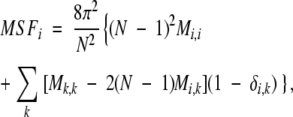(7)

and

(8)

where MSF_i is the mean squared fluctuation of atom i, RMSF_I is the root mean squared fluctuation of residue I, and n_I is the number of atoms in that residue.

Results and Discussion

We first test the method by using two small proteins: one all-α protein and one all-β protein. They are a 46-residue three-helix bundle protein fragment B of Staphylococcal protein A (Protein Data Bank [PDB] ID 1BDD) and a 56-residue α-spectrin SH3 domain protein (PDB ID 1SHG), respectively.

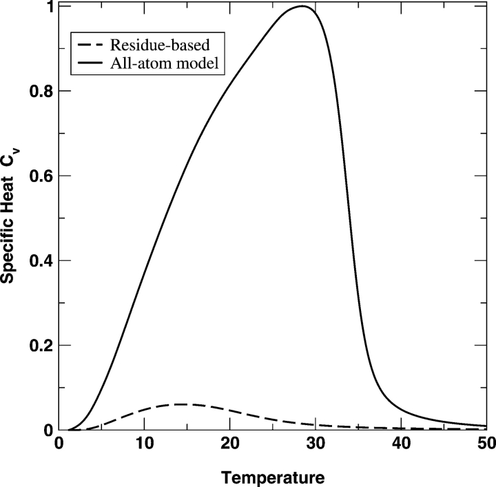
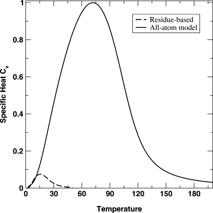
Figure 1 ▶ compares the specific heat capacity C_V given by the coarse-grained residue-level (C_α only) model and that by the all-atom model for fragment B of protein A. The peak height and area for the folding transition in the all-atom model are significantly higher (or larger) than that in the residue-based model. The folding transition temperature for the all-atom model is also much higher than that for the residue-based model. The similar feature is observed for the α-spectrin SH3 domain protein in Figure 2 ▶ as well. This result is in part due to significantly more interactions in the atomic model than in the residue-level model. It is also consistent with the finding that an all-atom model with specific packing yields a stronger transition than does a residue-based model (Zhou and Linhananta 2002). However, it is difficult to assess which model yields a more accurate C_V curve because the peaks in both curves are very broad. In contrast, a typical heat-capacity curve of proteins is much narrower, as a result of a first-order-like, cooperative folding transition (Privalov 1979; Zhou et al. 1999; Kaya and Chan 2003).

Figure 1.

The normalized specific heat capacity, C_V, as a function of the temperature T for the all-atom mean-field model (solid line) and for the residue-based model of the fragment B of Staphylococcal protein A. The C_V curves are normalized by the maximum value of C_V given by the all-atom model.

Figure 2.

As in Figure 1 ▶ but for the SH3 domain protein (1SHG).

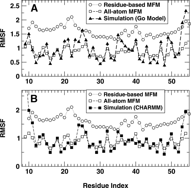
Figure 3 ▶ compares the RMSF values of fragment B of Staphylococcal protein A at T=5 predicted by residuebased and all-atom mean-field models (MFMs) with those from simulation studies of all-atom Go model– based square-well interactions (Zhou and Linhananta 2002) and from the all-atom CHARMM simulations in explicit water at 300 K (using all-atom CHARMM 22 parameter set; A. Linhananta and Y. Zhou, unpubl.). We used T=5 because at that temperature, the native structure is stable for both models. One can also use temperatures other than 5. We found that there is only a weak dependence of RMSF on temperature. As the figure shows, the all-atom model makes a substantially more accurate prediction in RMSF than does the residue-based model. There is a clearer separation of rigid and flexible residues in the all-atom model than in the residue-based model. Table 1 further shows that there is a significant correlation between the RMSF from the all-atom MFM and that from the simulation of either a Go model or a CHARMM model. The correlation coefficients are 0.78 and 0.64, respectively. In contrast, there is no significant correlation between the RMSF from the residue-level model and that from either simulation. Moreover, the result from mean-field Go model has a better correlation with the simulation result of a Go model than with the simulation result of a CHARMM model, as expected.

Figure 3.

The RMSF (in Å) for different residues. The results of residue-level model and all-atom mean-field model (with Go interactions) are compared with the results from simulations of the fragment B of Staphylococcal protein A with the Go model (A) and the CHARMM force field (B) in explicit water molecules.

Table 1.

The correlation coefficients between RMSF obtained from the mean-field theory with that from all-atom simulations (1BDD) or that from X-ray temperature B-factors

	1BDD
Mean-field model	Square-well Go modela	CHARMMb	1SHG X-rayc
Residue basedd	0.48	0.29	0.60
All-atome	0.78	0.64	0.79

^a From an all-atom molecular dynamics simulations of a square-well-chain model of 1BDD with the Go interaction. Data from Zhou and Linhananta (2002).

^b From an all-atom molecular dynamics simulations of 1BDD using the CHARMM force field. (A. Linhananta and Y. Zhou, unpubl.).

^c From temperature B-factors.

^d This work. Calculated from the mean-field residue-level (C_α only) model at T=5.

^e This work. Calculated from the all-atom mean-field model at T=5.

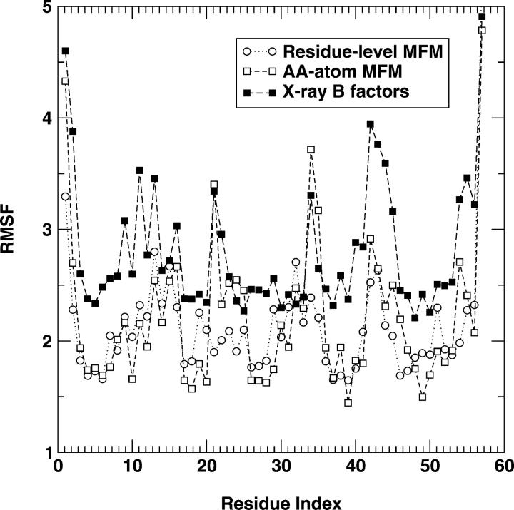
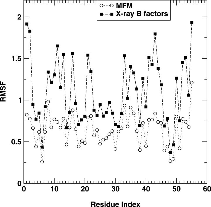
The RMSF for the α-spectrin SH3 domain protein at T=5 is shown in Figure 4 ▶. In this case, the difference between the results of a residue-based MFM and that of an all-atom model is not as large as in fragment B of Staphylococcal protein A but continues to be significant. There is a good correlation between the RMSF from the residue-based MFM and that from X-ray temperature B-factors with a correlation coefficient of 0.60. The use of all-atom model significantly improves the correlation from the correlation coefficient of 0.60 to 0.79 (Table 1).

Figure 4.

As in Figure 3 ▶ but for 1SHG.

It is of interest to know if a model beyond Go model would improve the agreement between the mean-field RMSF results and that from either simulations or experiments. To test this, we used the all-atom model with residue-based χ_i,j from Miyazawa-Jernigan (MJ) parameter set (Miyazawa and Jernigan 1985) and from Canino et al. (2002) (the latter was from Dasgupta et al. 1997). This is done by applying the residue-based parameter to all atoms in that residue. The correlation coefficient at T=5 for 1SHG is 0.79 between the results from the all-atom MFM with the MJ parameter set and the results from experiments, and 0.78 between the results from the all-atom MFM with the Dasgupta parameter set and the results from experiments. Thus, there is no obvious improvement from the use of residue- based energy parameters in the all-atom MFM. There is also no improvement at the residue level. The correlation coefficient at the residue-level model is 0.60 for the Go model and 0.58 for both the MJ and Dasgupta parameter sets. We also used the statistical atomic contact energy obtained by McConkey et al. (2003) for χ_i,j. However, we find that the correlation between predicted and experimental RMSF values becomes significantly worse. For example, the correlation coefficient is reduced from 0.79 to 0.60 for 1SHG at T=5. Clearly, there is a need to search for a different parameter set in order to further improve the accuracy of predicted flexibility by the all-atom MFM developed here.

The results reported above are only for two small-size proteins. We further test the all-atom mean-field theory for additional six all-α, three all-β, and three mixed α, β proteins. They were selected based on their relatively small sizes plus a few medium sizes. The protein PDB identifications, the sizes of proteins, and the experimental methods are listed in Table 2. In addition, this table shows the correlation coefficients between theoretically predicted (both residue-level and all-atom-level models) and experimentally measured RMSF values (based on temperature B-factors or fluctuation data from NMR experiments deposited in the PDB) along with their dependence on the cutoff distance that defined the native contact.

Table 2.

The correlation coefficients between experimentally measured and theoretical predicted RMSF values at different contact cutoff distances for 14 proteins

				Cutoff distance
Protein	Experimental methoda	Modelb	Sizec	6.5A °	10.5A °	14.5A °
1BDDd	NMR	AA	368	0.78	0.80	0.75
		RB	46	0.48	0.72	0.66
2ERLd	X-ray (1.0)	AA	303	0.61	0.77	0.79
		RB	40	0.71	0.80	0.77
1BW6d	NMR	AA	459	0.32	0.78	0.76
		RB	56	0.57	0.51	0.49
1EZ3d	X-ray (1.9)	AA	1023	0.44	0.77	0.80
		RB	124	0.50	0.45	0.74
1PRBd	NMR	AA	419	0.12	0.79	0.87
		RB	53	0.77	0.73	0.87
1CF7d	X-ray (2.6)	AA	525	0.06	0.30	0.29
		RB	67	0.10	0.09	0.09
1TNSd	NMR	AA	582	0.21	0.81	0.88
		RB	76	0.88	0.86	0.87
1SHGe	X-ray (1.8)	AA	472	0.79	0.81	0.79
		RB	56	0.60	0.71	0.65
1IBYe	X-ray (1.65)	AA	863	0.58	0.73	0.76
		RB	112	0.50	0.71	0.75
1BOWe	X-ray (1.8)	AA	840	0.33	0.68	0.67
		RB	108	0.50	0.45	0.44
1VGEe	X-ray (2.0)	AA	1632	0.49	0.58	0.57
		RB	214	0.44	0.38	0.62
1COAf	X-ray (2.2)	AA	512	0.17	0.64	0.60
		RB	64	0.32	0.30	0.51
1DIVf	X-ray (2.6)	AA	1148	0.32	0.39	0.46
		RB	149	0.14	0.08	0.06
2VIKf	NMR	AA	997	0.28	0.78	0.80
		RB	126	0.65	0.78	0.82

^a Resolution in Ångstroms.

^bAA and RB denote the all-atom and residue-based mean-field models, respectively.

^c The number of heavy atoms (for all-atom, AA model) or residues (for residue-based, RB model).

^d α-Proteins. Calculated at T=5.

^e β-Proteins. Calculated at T=5.

^f Mixed α, β-proteins. Calculated at T=5.

Such a more extensive study reveals that the accuracy of flexibility prediction is strongly dependent on the cutoff distance that defines the contact. For example, the difference in accuracy between the all-atom model and the residue-level model of the three-helix bundle protein fragment B of Staphylococcal protein A is not as drastic as shown in Figure 3 ▶. A larger value of the distance cutoff significantly improves the correlation coefficient between the residue-based MFM and the simulation result from 0.48 (at 6.5 Å) to 0.72 (at 10.5 Å). The all-atom model further improves the correlation from 0.72 to 0.80 (at a cutoff distance of 10.5 Å). This improvement is closer to the improvement in prediction of RMSF values of SH3 domain by the all-atom model to that by the residue-based model (Fig. 4 ▶).

A more detailed examination of Table 2 indicates that a large value of contact cutoff is required for a more accurate prediction of flexibility by the all-atom MFM, in general. In fact, if a cutoff distance of 6.5 Å is used, the all-atom model provides a more accurate prediction than does the residue-based model only in five out of 14 proteins (based on the correlation coefficients). Only at a larger cutoff value (e.g., 10.5 Å or 14.5 Å), the all-atom model becomes more accurate in most cases (11 out of 14 cases at 10.5 Å and 14.5 Å). It is not entirely clear why a longer cutoff distance is required for a more accurate prediction of flexibility in the all-atom model. A similar situation was observed in the anisotropic network model (Atilgan et al. 2001), where it was found that a large cutoff value (12–15 Å) is required in order to remove certain unphysical behavior of the model. One possibility is that one may have to go beyond the first coordination shell around a residue (about 6.5 Å) (Bahar et al. 1997) for a better estimate of the interactions in proteins as a result of long-range electrostatic interactions. On the other hand, the large cutoff value may be the result of compensation for the crude approximation of the atomic interactions in the all-atom MFM.

While flexibilities for majority of proteins studied here are predicted in a reasonable accuracy, there are no significant correlations at any cutoff distances for two proteins (1CF7 and 1DIV) either by residue-based or all-atom MFMs. The two proteins happen to be the lowest resolution (2.6 Å) proteins among the nine proteins whose structures are solved by the X-ray crystallographic method. A close examination of Table 2 further indicates the trend of a lower correlation coefficient accompanied with a lower resolution.

To minimize the effect of structural inaccuracy on flexibility prediction, we tested the all-atom MFM and residue-level MFM on six additional, randomly selected proteins with high resolutions (≤1 Å). They are one all-α, one all-β, and four mixed α, β proteins with the number of residues ranging from 63 to 151. The correlation coefficients are shown in Table 3. The overall result is similar to the one given in Table 2. That is, the all-atom model provides the best flexibility prediction at large cutoff distances (10.5 Å and 14.5 Å) among the three models in six out of six cases.

Table 3.

The correlation coefficients between experimentally measured and theoretical predicted RMSF values at different contact cutoff distances for six proteins with higher-solution protein structures (≤1 Å)

				Cutoff distance
Protein	Experimental methoda	Modelb	Sizec	6.5A °	10.5A °	14.5A °
1A6Md	X-ray (1.0)	AA	1204	0.41	0.85	0.86
		RB	151	0.59	0.58	0.66
1F94e	X-ray (0.97)	AA	516	0.72	0.84	0.85
		RB	63	0.59	0.33	0.28
1AHOf	X-ray (0.96)	AA	500	0.55	0.89	0.92
		RB	64	−0.29	−0.21	−0.12
1BYIf	X-ray (0.97)	AA	1692	0.41	0.81	0.80
		RB	224	0.54	0.50	0.45
1C7Kf	X-ray (1.0)	AA	1015	0.20	0.80	0.83
		RB	132	0.54	0.63	0.62
1EB6f	X-ray (1.0)	AA	1338	0.45	0.86	0.90
		RB	177	0.50	0.63	0.66

^a Resolution in Ångstroms.

^bAA and RB denote the all-atom and residue-based mean-field models, respectively.

^c The number of heavy atoms (for all-atom, AA model) or residues (for residue-based, RB model).

^d α-Proteins. Calculated at T=5.

^e β-Proteins. Calculated at T=5.

^f Mixed α, β-proteins. Calculated at T=5.

One important feature of the all-atom model developed here is that it is able to predict the flexibility of the side-chains of amino acid residues as well. We found that the accuracy of side-chain flexibility predicted by the all-atom model is similar to that of residue flexibility by the same model (Results not shown). In Figure 5 ▶, the side-chain flexibilities predicted by the all-atom MFM are compared with those obtained from X-ray temperature B-factors for the α-spectrin SH3 domain protein at T=5 with a contact cutoff distance of 14.5 Å. A significant correlation between the two sets of data is observed with a correlation coefficient of 0.87.

Figure 5.

As in Figure 3 ▶ but for the comparison between side-chain flexibilities of 1SHG with a cutoff distance of 14.5 Å.

Summary

A mean-field-like method has been extended from a coarse-grained residue-level to the all-atom detail. We find that the all-atom detail leads not only to a stronger fold transition but also to a more accurate prediction of flexibility of residues in proteins. This result is based on study of two proteins—one all-α and one all-β proteins. Further application to 18 additional proteins indicates that predicted protein flexibility is reasonably accurate for majority of proteins studied (high-resolution proteins, in particular). Thus, an efficient and accurate prediction of protein flexibility is possible based on known protein structures and the positions of backbone and side-chains are both important for an accurate prediction.

Article and publication are at http://www.proteinscience.org/cgi/doi/10.1110/ps.041311005.

References

- Atilgan, A.R., Durell, S.R., Jernigan, R.L., Demirel, M.C., Keskin, O., and Bahar, I. 2001. Anisotropy of fluctuation dynamics of proteins with an elastic network model. Biophys. J. 80 505–515. [DOI] [PMC free article] [PubMed] [Google Scholar]
- Bahar, I., Atilgan, A.R., and Erman, B. 1997. Direct evaluation of thermal fluctuations in proteins using a single parameter harmonic potential. Fold. Des. 2 173–181. [DOI] [PubMed] [Google Scholar]
- Brooks, B.R., Bruccoleri, R.E., Olafson, B.D., States, D.J., Swaminathan, S., and Karplus, M. 1983. CHARMM: A program for macromolecular energy, minimization, and dynamics calculations. J. Comput. Chem. 4 187–217. [Google Scholar]
- Brooks III, C.L., Karplus, M., and Pettitt, B.M. 1988. Proteins: A theoretical perspective of dynamics, structure, and thermodynamics. John Wiley & Sons, New York.
- Canino, L.S., Shen, T.Y., and McCammon, J.A. 2002. Changes in flexibility upon binding: Application of the self-consistent pair contact probability method to protein–protein interactions. J. Chem. Phys. 117 9927–9933. [Google Scholar]
- Dasgupta, S., Iyer, G.H., Lawrence, S.H., and Bell, J.A. 1997. Extent and nature of contacts between protein molecules in crystal lattices and between subunits of protein oligomers. Proteins 28 494–514. [DOI] [PubMed] [Google Scholar]
- Doruker, P., Atilgan, A.R., and Bahar, I. 2000. Dynamics of proteins predicted by molecular dynamics simulations and analytical approaches: Application to α-amylase inhibitor. Proteins 40 512–524. [PubMed] [Google Scholar]
- Jacobs, D.J., Rader, A.J., Kuhn, L.A., and Thorpe, M.F. 2001. Protein flexibility prediction using graph theory. Proteins 44 150–165. [DOI] [PubMed] [Google Scholar]
- Kaya, H. and Chan, H. 2003. Simple two-state protein folding kinetics requires near-Levinthal thermodynamic cooperativity. Proteins 52 510–523. [DOI] [PubMed] [Google Scholar]
- McConkey, B.J., Sobolev, V., and Eldman, M. 2003. Discrimination of native protein structures using atom–atom contact scoring. Proc. Natl. Acad. Sci. 100 3215–3220. [DOI] [PMC free article] [PubMed] [Google Scholar]
- Micheletti, C., Banavar, J.R., and Maritan, A. 2001. Conformations of proteins in equilibrium. Phys. Rev. Lett. 87 088102. [DOI] [PubMed] [Google Scholar]
- Micheletti, C., Cecconi, F., Flammini, A., and Maritan, A. 2002. Crucial stages of protein folding through a solvable model: Predicting target sites for enzyme-inhibiting drugs. Protein Sci. 11 1878–1887. [DOI] [PMC free article] [PubMed] [Google Scholar]
- Micheletti, C., Carloni, P., and Maritan, A. 2004. Accurate and efficient description of protein vibrational dynamics: Comparing molecular dynamics and Gaussian models. Proteins 55 635–645. [DOI] [PubMed] [Google Scholar]
- Miyazawa, S. and Jernigan, R. 1985. Estimation of effective interresidue contact energies from protein crystal structures: Quasi-chemical approximation. Macromole 18 534–552. [Google Scholar]
- Privalov, P.L. 1979. Stability of proteins: Small globular proteins. Adv. Protein Chem. 33 167–241. [DOI] [PubMed] [Google Scholar]
- Shen, T., Canino, L.S., and McCammon, J.A. 2002. Unfolding proteins under external forces: A solvable model under the self-consistent pair contact probability approximation. Phys. Rev. Lett. 89 068103. [DOI] [PubMed] [Google Scholar]
- Taketomi, H., Ueda, Y., and Go, N. 1975. Studies on protein folding, unfolding and fluctuations by computer simulations. Int. J. Peptide Protein Res. 7 445–459. [PubMed] [Google Scholar]
- Ueda, Y., Taketomi, H., and Go, N. 1978. Studies on protein folding, unfolding and fluctuations by computer simulations, II: A three-dimensional lattice model of lysozyme. Biopolymers 17 1531–1548. [Google Scholar]
- Zhou, Y. and Linhananta, A. 2002. Thermodynamics of an all-atom off-lattice model of the fragment B of staphylococcal protein A: Implication for the origin of the cooperativity of protein folding. J. Phys. Chem. B 106 1481–1485. [Google Scholar]
- Zhou, Y., Hall, C.K., and Karplus, M. 1999. The calorimetric criterion for a two-state process revisited. Protein Sci. 8 1064–1074. [DOI] [PMC free article] [PubMed] [Google Scholar]