Probing the limits to positional information

Abstract

The reproducibility and precision of biological patterning is limited by the accuracy with which concentration profiles of morphogen molecules can be established and read out by their targets. We consider four measures of precision for the Bicoid morphogen in the Drosophila embryo: The concentration differences that distinguish neighboring cells, the limits set by the random arrival of Bicoid molecules at their targets (which depends on absolute concentration), the noise in readout of Bicoid by the activation of Hunchback, and the reproducibility of Bicoid concentration at corresponding positions in multiple embryos. We show, through a combination of different experiments, that all of these quantities are ~10%. This agreement among different measures of accuracy indicates that the embryo is not faced with noisy input signals and readout mechanisms; rather the system exerts precise control over absolute concentrations and responds reliably to small concentration differences, approaching the limits set by basic physical principles.

INTRODUCTION

The macroscopic structural patterns of multicellular organisms have their origins in spatial patterns of morphogen molecules (Wolpert 1969, Lawrence 1992). Translating this qualitative picture into quantitative terms raises several difficulties. First is the problem of precision (Figure 1): Neighboring cells often adopt distinct fates, but the signals that drive these decisions involve very small differences in morphogen concentration, and these must be discriminated against the inevitable background of random noise. The second problem is reproducibility: If cells “know” their location based on the concentration of particular morphogens, then generating reproducible final patterns requires either that the absolute concentrations of these molecules be reproducible from embryo to embryo or that there exist mechanisms which achieve a robust output despite variable input signals. These problems of precision and reproducibility are potentially relevant to all biochemical and genetic networks, and analogous problems of noise (de Vries 1957; Barlow 1981; Bialek 1987, 2002) and robustness (LeMasson et al 1993; Goldman et al 2001) have long been explored in neural systems. Here we address these issues in the context of the initial events in fruit fly development.

FIG. 1.

Schematic of the readout problem for the Bicoid gradient. At left, the conventional picture. A smooth gradient of Bcd concentration is translated into a sharp boundary of Hb expression because Bcd acts as a cooperative activator of the hb gene. Although intended as a sketch, the different curves have been drawn to reflect what is known about the scales on which both the Bcd and Hb concentrations vary. Note that neighboring cells along the anterior-posterior axis experience Bcd concentrations that are very similar (differing by ~ 10%, as explained in the text), yet the resulting levels of Hb expression are very different. At right, we consider a larger number of cells in the mid-embryo region where Hb expression switches from high to low values. From direct experiments on simpler systems we know that, even when the concentrations of transcription factors are fixed, the resulting levels of gene expression will fluctuate (Elowitz et al 2002; Raser & O’Shea 2004), and there are physical limits to how much this noise can be reduced (Bialek & Setayeshgar 2005, 2006). If the noise is low, such that a scatter plot of Hb expression vs Bcd concentration is relatively tight, then the qualitative picture of a sharp Hb expression boundary is perturbed only slightly. If the noise is large, so that there is considerable scatter in the relationship between Bcd and Hb measured for individual cells, then the sharp Hb expression boundary will exist only on average, and not along individual rows in individual embryos.

The primary determinant of patterning along the anterior-posterior axis in the fly Drosophila melanogaster is the gradient of Bicoid (Bcd), which is established by maternal placement of bcd mRNA at the anterior end of the embryo (Driever & Nüsslein-Volhard 1988a,b); Bcd acts as a transcription factor, regulating the expression of hunchback (hb) and other downstream genes (Struhl et al 1989; Rivera-Pomar et al 1995; Gao & Finkelstein 1998). This cascade of events generates a spatial pattern so precise that neighboring nuclei have readily distinguishable levels of expression for several genes [as reviewed by Gergen et al (1986)], and these patterns are reproducible from embryo to embryo (Crauk & Dostatni 2005; Holloway et al 2006).

In trying to quantify the precision and reproducibility of the initial events in morphogenesis, we can ask four conceptually distinct questions:

• If cells make decisions based on the concentration of Bcd alone, how accurately must they “measure” this concentration to be sure that neighboring cells reach reliably distinguishable decisions?

• What is the smallest concentration difference that can be measured reliably, given the inevitable noise that results from random arrival of individual Bcd molecules at their target sites along the genome?

• What level of precision does the system actually achieve, for example in the transformation from Bcd to Hb?

• How reproducible are the absolute Bcd concentrations at corresponding locations in different embryos?

The answer to the first question just depends on the spatial profile of Bicoid concentration (Houchmandzadeh et al 2002). To answer the second question we need to know the absolute concentration of Bcd in nuclei, and we measure this using the Bcd-GFP fusion constructs described in a companion paper (Gregor et al 2007). To answer the third question we characterize directly the input/output relation between Bcd and Hb protein levels in each nucleus of individual embryos. Finally, to answer the fourth question we make absolute concentration measurements on many embryos, as well as using more classical antibody staining methods. In the end, we find that all of these questions have the same answer: ~ 10% accuracy in the Bcd concentration. While this number is interesting, it is the agreement among the four different notions of precision that we find most striking.

A number of previous groups have argued that the central problem in thinking quantitatively about the early events in development is to understand how an organism makes precise patterns given sloppy initial data and noisy readout mechanisms (von Dassow et al 2000; Houchmandzadeh et al 2002; Spirov et al 2003; Jaeger et al 2004; Eldar et al 2004; Martinez Arias & Hayward, 2006; Holloway et al 2006). In contrast, our results lead us to the problem of understanding how extreme precision and reproducibility–down to the limits set by basic physical principles–are achieved in the very first steps of pattern formation.

RESULTS

Setting the scale

Two to three hours after fertilization of the egg, adjacent cells have adopted distinct fates, as reflected in their patterns of gene expression. At this stage, the embryo is ~ 500 μm long and neighboring nuclei are separated by Δx ~ 8 μm. Distinct fates in neighboring cells therefore means that they acquire positional information with an accuracy of ~ 1 – 2% along the anterior-posterior axis. Measurements of Bcd concentration by immunostaining reveal an approximately exponential decay along this axis, c(x) = c₀ exp(−x/λ), with a length constant λ ~ 100 μm (Houchmandzadeh et al 2002). Neighboring nuclei, at locations x and x + Δx, thus experience Bcd concentrations which differ by a fraction

$$\frac{\mathrm{\Delta }c(x)}{c(x)}=\frac{1}{c(x)}\mid \frac{dc(x)}{dx}\mid \mathrm{\Delta }x=\frac{\mathrm{\Delta }x}{\lambda }~\mathrm{0.1.}$$ (1)

To distinguish individual nuclei from their neighbors reliably using the Bcd morphogen alone there-fore would require each nucleus to “measure” the Bcd concentration with an accuracy of ~ 10%.

Absolute concentrations

The difficulty of achieving precise and reproducibly functioning biochemical networks is determined in part by the absolute concentration of the relevant molecules: for sufficiently small concentrations, the randomness of individual molecular events must set a limit to precision (Berg & Purcell 1977; Bialek & Setayeshgar 2005, 2006). Since Bcd is a transcription factor, what matters is the concentration in the nuclei of the forming cells. A variety of experiments on Bcd (Ma et al 1996; Burz et al 1998; Zhao et al 2002) and other transcription factors (Ptashne 1992; Pedone et al 1996; Winston et al 1999) suggest that they are functional in the nanoMolar range, but to our knowledge there exist no direct in vivo measurements in the Drosophila embryo.

In Figure 2A we show an optical section through a live Drosophila embryo that expresses a fully functional fusion of the Bcd protein with the green fluorescent protein, GFP (Gregor et al 2007). of the native Bcd. In scanning two-photon microscope images we identify individual nuclei to measure the mean fluorescence intensity in each nucleus, which should be proportional to the protein concentration. To establish the constant of proportionality we bathe the embryo in a solution of purified GFP with known concentration and thus compare fluorescence levels of the same moiety under the same optical conditions (see Methods).

FIG. 2.

Absolute concentration of Bcd. A: Scanning two-photon microscope image of a Drosophila embryo expressing a Bcd-GFP fusion protein (Gregor et al 2007); scale bar 50 μm. The embryo is bathed in a solution of GFP with concentration 36 nM. We identify individual nuclei and estimate the mean Bcd-GFP concentration by the ratio of fluorescence intensity to this standard. B: Apparent Bcd-GFP concentrations in each visible nucleus plotted vs. anterior-posterior position x (reference line in A) in units of the egg length L; red and blue points are dorsal and ventral, respectively. Repeating the same experiments on wild type flies which do not express GFP, we find a background fluorescence level shown by the black points with error bars (standard deviation across four embryos). In the inset we subtract the mean background level to give our best estimate of the actual Bcd-GFP concentration in the nuclei near the midpoint of the embryo. Points with error bars show the nominal background, now at zero on average.

Some of the observed fluorescence is contributed by molecules other than the Bcd-GFP, and we estimate this background by imaging wild type embryos under exactly the same conditions. As shown in Figure 2B, this background is almost spatially constant and essentially equal to the level seen in the Bcd-GFP flies at the posterior pole, consistent with the idea that the Bcd concentration is nearly zero at this point.

Figure 2B shows the concentration of Bcd-GFP in nuclei as a function of their position along the anterior-posterior axis. The maximal concentration near the anterior pole, corrected for background, is c_max = 55 ± 3 nM, while the concentration in nuclei near the mid-point of the embryo, near the threshold for activation of hb expression (at a position x/L ~ 48% from the anterior pole), is c = 8 ± 1 nM. This is close to the disassociation constants measured in vitro for binding of Bcd to its target sequences in the hb enhancer (Ma et al 1996; Burz et al 1998; Zhao et al 2002).

Physical limits to precision

Our interest in the precision of the readout mechanism for the Bcd gradient is heightened by the theoretical difficulty of achieving precision on the ~10% level. To begin, note that 1 nM corresponds to 0.6 molecules/μm³, so that the concentration of Bcd in nuclei near the midpoint of the embryo is c = 4.8 ± 0.6 molecules/μm³, or 690 total molecules in the nucleus during nuclear cycle 14. A ten percent difference in concentration thus amounts to changes of ~ 70 molecules.

Berg and Purcell (1977) emphasized, in the context of bacterial chemotaxis, that the physical limit to concentration measurements is set not by the total number of available molecules, but by the dynamics of their random arrival at their target locations. Consider a receptor of linear size a, and assume that the receptor occupancy is integrated for a time T. Berg and Purcell argued that the precision of concentration measurements is limited to

$$\frac{\delta c}{c}~\frac{1}{\sqrt{\mathit{DacT}}},$$ (2)

where c is the concentration of the molecule to which the system is responding and D is its diffusion constant in the solution surrounding the receptor. Recent work shows that the Berg-Purcell result really is a lower limit to the noise level (Bialek & Setayeshgar 2005, 2006): the complexities of the kinetics describing the interaction of the receptor with the signaling molecule just add extra noise, but cannot reduce the effective noise level below that in Equation (2). These theoretical results encourage us to apply this formula to understand the sensitivity of cells not just to external chemical signals (as in chemotaxis) but also to internal signals, including morphogens such as Bcd.

Here we estimate the parameters that set the limiting accuracy in Equation (2); for details see Supplemental Data. The total concentration of Bcd in nuclei is c = 4.8 ± 0.6 molecules/μm³ near the point where the “decision” is made to activate Hb (Figure 2B). Bicoid diffuses slowly through the dense cytoplasm surrounding the nuclei with a diffusion constant D < 1 μm²/s (Gregor et al 2007), which is similar to that observed in bacterial cells (Elowitz et al 1999), and we take this as a reasonable estimate of the effective diffusion constant for Bcd in the nucleus. Receptor sites for eukaryotic transcription factors are ~ 10 base pair segments of DNA with linear dimensions a ~ 3 nm. The remaining parameter, which is unknown, is the amount of time T over which the system averages in determining the response to the Bcd gradient; the longer the averaging time the lower the noise level. Putting together the parameters above, we have

$$\frac{\delta c}{c}~{[\mathit{DacT}]}^{-1/2}={[(1\hspace{0.17em}\mu {\mathrm{m}}^2/\mathrm{s})\hspace{0.17em}(3\hspace{0.17em}\mathrm{nm})\hspace{0.17em}(4.8/\mu {\mathrm{m}}^3)T]}^{-1/2}~{\left(\frac{70\hspace{0.17em}\mathrm{s}}{T}\right)}^{1/2}.$$ (3)

Thus to achieve precision on the ~10% level, i.e. δc/c ~ 0.1, requires T ~ 7000 s, or nearly two hours. This is almost the entire time available for development from fertilization up to cellularization, and it seems implausible that downstream gene expression levels reflect an average of local Bcd concentrations over this long time, especially given the enormous changes in local Bcd concentration during the course of each nuclear cycle (Gregor et al 2007).

Our discussion ignores all noise sources other than the fundamental physical process of random molecular arrivals at the relevant binding sites; additional noise sources would necessitate even longer averaging times. Although there are uncertainties, the minimum time required to push the physical limits down to the ~10% level seems inconsistent with the pace of developmental events.

Input/output relations and noise

The fact that neighboring cells can generate distinct patterns of gene expression does not mean that any single step in the readout of the primary morphogen gradients achieves this level of precision. Here we measure more directly the precision of the transformation from Bcd to Hb, one of the first steps in the generation of anterior-posterior pattern.

In Figure 3A we show confocal microscope images of a Drosophila embryo fixed during nuclear cycle 14 and immunostained for DNA, Bcd and Hb; the fluorescence peaks of the different labels are sufficiently distinct that we can obtain independent images of the three stains. The DNA images allow us to locate automatically the centers and outlines of the ~ 1200 nuclei in a single image of one embryo (see Methods). Given these outlines we can measure the average intensity of Bcd and Hb staining in each nucleus (Figure 3B). We have shown in a companion paper (Gregor et al 2007) that immunofluorescent staining intensity I is proportional to protein concentration c plus some non-specific background: I = Ac + B, where A and B are constant in a single image. With this linearity, a single image provides more than 1000 points on the scatter plot of Hb expression level vs Bcd concentration, as in Figure 3C.

FIG. 3.

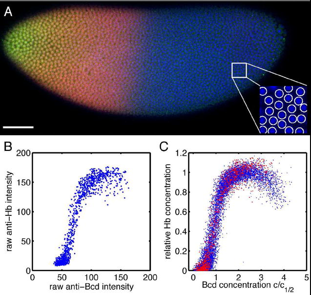
Hb vs. Bcd concentrations from fixed and stained embryos. A: Scanning confocal microscope image of a Drosophila embryo in early nuclear cycle 14, stained for DNA (blue), Hb (red) and Bcd (green); scale bar 50 μm. Inset (28×28 μm²) shows how DNA staining allows for automatic detection of nuclei (see Methods). B: Scatter plot of Hb vs Bcd immunofluorescent staining levels from 1299 identified nuclei in a single embryo. C: Scatter plot of Hb vs Bcd concentration from a total of 13,366 nuclei in 9 embryos, normalized (see Methods). Data from the single embryo in B are highlighted.

Scatter plots as in Figure 3 contain information both about the mean “input/output” relation between Bcd and Hb and about the precision or reliability of this response. We can think of these data as the generalization to multicellular, eukaryotic systems of the input/output scatter plots measured for engineered regulatory elements in bacteria [e.g. Figure 3B of Rosenfeld et al (2005)]. To analyze these data we discretize the Bcd axis into bins, grouping together nuclei which have very similar levels of staining for Bcd; within each bin we compute the mean and variance of the Hb intensity. We measure the Hb level in units of its maximal mean response, and the Bcd level in units of the level which generates (on average) half maximal Hb.

Input/output relations between Bcd and Hb are shown for nine individual embryos in Figure 4A. Results from different embryos are very similar (see Methods for discussion of normalization across embryos), and pooling the results from all embryos yields an input/output relation that fits well to the Hill relation,

FIG. 4.

Input/output relations and noise. A: Mean input/output relations for 9 embryos. Curves show the mean level of Hb expression as a function of the Bcd concentration, where we use a logarithmic axis to provide a clearer view of the steep, sigmoidal nonlinearity. Points and error bars show, respectively, the mean Hb level and standard deviation of the output noise for one of the embryos. Inset shows mean Hb output (points) and standard errors of the mean (error bars) when data from all embryos are pooled. The mean response is consistent with the Hill relationship, Equation (4), with n = 5, corresponding to a model in which five Bcd molecules bind cooperatively to activate Hb expression (red line). In comparison, Hill relations with n = 3 or n = 7 provide substantially poorer fits to the data (green lines). B: Standard deviations of Hb levels for nuclei with given Bcd levels. C: Translating the output noise of (B) into an equivalent input noise, following Equation (6). Blue dots are data from 9 embryos, green line with error bars is an estimate of the noise in our measurements (see Methods), and red circles with error bars are results after correcting for measurement noise. D: Correlation function of Hb output noise, normalized by output noise variance, as a function of distance r measured in units of the mean spacing ℓ between neighboring nuclei. Lines are results for four individual embryos, points and error bars are the mean and standard deviation of these curves. We have checked that the dominant sources of measurement noise are uncorrelated between neighboring nuclei. The large difference between r = 0 and r = ℓ arises largely from this measurement noise. Inset shows the same data on a logarithmic scale, with a fit to an exponential decay C ∝ exp(−r/ξ); the correlation length ξ/ℓ = 5 ± 1.

$$\mathrm{Hb}={\mathrm{Hb}}_{\max }\frac{{\mathrm{Bcd}}^n}{{\mathrm{Bcd}}^n+{\mathrm{Bcd}}_{1/2}^n}.$$ (4)

The best fit is with n = 5, consistent with the idea that Hb transcription is activated by cooperative binding of effectively five Bcd molecules, as expected from the identification of seven Bcd binding sites in the hb promoter (Struhl et al 1989; Driever & Nüsslein-Volhard 1989).

In Figure 4B we show the standard deviation in Hb levels as a function of the Bcd concentration. Output fluctuations are below 10% when the activator Bcd is at high concentration, similar to results on engineered systems (Elowitz et al 2002; Raser & O’Shea 2004). If we think of the Hb expression level as a readout of the Bcd gradient, then we can convert the output noise in Hb levels into an equivalent level of input noise in the Bcd concentration. This is the same transformation as for the propagation of errors: we ask what level of error δc in Bcd concentration would generate the observed level of variance in Hb expression,

$${\sigma }_{\mathrm{Hb}}^2(\mathrm{Bcd})={\mid \frac{d[\mathrm{Hb}]}{d[\mathrm{Bcd}]}\mid }^2{(\delta c)}^2,$$ (5)

or

$$\frac{\delta c}{c}={\sigma }_{\mathrm{Hb}}(\mathrm{Bcd}){\mid \frac{d[\mathrm{Hb}]}{d\hspace{0.17em}\ln [\mathrm{Bcd}]}\mid }^{-1}.$$ (6)

It is this equivalent fractional noise level (Figure 4C) that cannot fall below the physical limit set by Equation (2). For individual embryos we find a minimum value of δc/c ~ 0.1 near c = c_1/2.

It should be emphasized that all of the noise we observe could in principle result from our measurements. In particular, because the input/output relation is very steep, small errors in measuring the Bcd concentration will lead to a large apparent variance of the Hb output. In separate experiments (see Methods) we estimate the component of measurement noise which arises in the imaging process. Subtracting this instrumental variance results in values of δc/c ~ 0.1 on average (circle with error bars in Figure 4C). The true noise level could be even lower, since we have no way of correcting for nucleus-to-nucleus variability in the staining process.

Before proceeding it is important to emphasize the limitations of our analysis. We have treated the relationship between Bcd and Hb as if there were no other factors involved. In the extreme one could imagine (although this is not true) that both Bcd and Hb concentrations vary with anterior-posterior position in the embryo, but are not related causally. In fact, if we look along the dorsal-ventral axis, there are systematic variations in Bcd concentration (cf Figure 3), and the Hb concentrations are correlated with these variations, suggesting that Bcd and Hb really are linked to each other rather than to some other anterior-posterior position signal. It has been suggested, however, that hb expression may be responding to signals in addition to Bcd (Howard & ten Wolde 2005; Houchmandzadeh et al 2005; McHale et al 2006). If these signals ultimately are driven by the local Bcd concentration itself, then it remains sensible to say that the Hunchback concentration provides a readout of Bcd concentration with an accuracy of ~ 10%. If additional signals are not correlated with the local Bcd concentration, then collapsing our description into an input/output relation between Bcd and Hb treats these other variables as an extrinsic source of noise; the intrinsic reliability of the transformation from Bcd to Hb would have to be even better than what we observe.

Noise reduction by spatial averaging?

The observed precision of ~ 10% is difficult to reconcile with the physical limits [Equation (3)] given the available averaging time. If the precision cannot be increased to the observed levels by averaging over time, perhaps the embryo can achieve some averaging over space: If the Hb level in one nucleus reflects the average Bcd levels in its N neighbors, the limiting noise level in Equation (3) should decrease by a factor of $\sqrt{N}$.

If communication among nuclei is mediated by diffusion of a protein with diffusion constant comparable to that of Bcd itself, then in a time T it will cover a radius $r~\sqrt{4DT}$ and hence an area A ~ 4πDT. But at cycle 14 the nuclei form an approximately regular lattice of triangles with side ℓ ~ 8.5 μm, so the area A contains

$$N~\frac{8\pi }{\sqrt{3}}\frac{DT}{{\ell }^2}$$ (7)

nuclei. Putting all the factors together, in just four minutes it should be possible to average over roughly 50 nuclei. Since averaging over time and averaging over nuclei have the same effect on the noise level, averaging over fifty nuclei for four minutes is the same as each nucleus acting independently but averaging for two hundred minutes. More generally, with communication among nuclei the physical limit becomes

$$\frac{\delta c}{c}~\frac{1}{\sqrt{\mathit{DacTN}}}={\left[\frac{\sqrt{3}}{8\pi ac}\right]}^{1/2}\frac{\ell }{DT}~\frac{20\mathrm{s}}{T}.$$ (8)

Thus 10% precision is possible with mechanisms that integrate for only ~ 200 s, or ~ 3 minutes—within a single nuclear cycle—rather than hours.

If each nucleus makes independent decisions, then noise in the Hb levels of individual nuclei should be independent. But if Hb expression reflects an average over the nuclei in a neighborhood, then noise levels necessarily become correlated within this neighborhood. Going back to our original images of Bcd and Hb levels, we can ask how the Hb level in each nucleus differs from the average (along the input/output relation of Figure 4A) given its Bcd level, and we can compute the correlation function for this array of Hb noise fluctuations (see Methods). The results, shown in Figure 4D, reveal a component with a correlation length ξ= 5 ± 1 nuclei, as predicted if averaging occurs on the scale required to suppress noise.

Reproducibility in live embryos

Figure 4 shows that individual embryos can “read” the profile of Bcd concentration with an accuracy of ~ 10%, so that the Bcd concentration has a precise meaning within each embryo. Is this meaning invariant from embryo to embryo? Such a scenario would require control mechanisms to insure reproducibility of the absolute copy numbers of Bcd and other relevant gene products. Alternatively, spatial profiles of Bcd could vary from embryo to embryo, but other mechanisms allow for a robust response to this variable input. A number of groups have argued for the latter scenario (von Dassow et al 2000; Houchmandzadeh et al 2002; Spirov et al 2003; Jaeger et al 2004; Howard & ten Wolde 2005; Holloway et al 2006). In contrast, the similarity of Bcd/Hb input/output relations across embryos (Figure 4A) suggests that reproducible outputs result from reproducible inputs.

To measure the reproducibility of the Bcd gradient, we use live imaging of the Bcd-GFP fusion construct, as in Figure 2. To minimize variations in imaging conditions, we collect several embryos that are approximately synchronized and mount them together in a scanning two-photon microscope. Nucleus-by-nucleus profiles of the Bcd concentration during the first minutes of nuclear cycle 14 are shown for 15 embryos in Figure 5A (see Methods). Qualitatively it is clear that these profiles are very similar across all embryos. We emphasize that these comparisons require no scaling or separate calibration of images for each embryo; one can compare raw data, or with one global calibration (as in Figure 2) we can report these data in absolute concentration units.

FIG. 5.

Reproducibility of the Bcd profile in live embryos. A: Bcd-GFP profiles of 15 embryos. Each dot represents the average concentration in a single nucleus at the mid-sagittal plane of the embryo (on average 70 nuclei per embryo). All nuclei from all embryos are binned in 50 bins, over which the mean and standard deviation were computed (black points with error bars). Scale at left shows raw fluorescence intensity, and at right we show concentration in nM, with background subtracted, as in Figure 2. B: For each bin from A, standard deviations divided by the mean as a function of fractional egg length (blue); errorbars are computed by bootstrapping with 8 embryos. Grey and black lines show estimated contributions to measurement noise (see Methods). C: Variability of Bcd profiles translated into an effective rms error σ(x) in positional readout, as in Equation (9); error bars from bootstrapping. Green circles are obtained by correcting for measurement noise. D: Bcd-GFP profiles of 3 embryos expressing 2 copies of Bcd-GFP (red) and of 3 embryos expressing 1 copy of Bcd-GFP (blue). Each dot represents a single nucleus as in A. In green, we show fluorescence intensities from 1X embryos multiplied by two, after background correction. E: 2X vs. 1X Bcd-GFP profiles–no normalization, all possible permutations (blue dots). Red line represents a linear fit to all data points, $(I_{\mathit{nuc}}^{2\mathrm{X}}=1.95I_{\mathit{nuc}}^{1\mathrm{X}}-41.8)$, where the offset corresponds to the imaging background.

We quantify the variability of Bcd levels across embryos by measuring the (fractional) standard deviation of concentration across nuclei at similar locations in different embryos. The results, shown in Figure 5B, are consistent with reproducibility at the 10–20% level across the entire anterior half of the embryo, with variability gradually rising in the posterior half where Bcd concentrations are much lower. Thus the reproducibility of the Bcd profile across embryos is close to precision with which it can be read out within individual embryos. At the anterior end of the egg, the absolute variability is somewhat greater and may reflect a requirement for additional signaling systems in this region (e. g., torso) if cell fates need to be determined with comparable accuracy (see Supplemental Data).

The average concentration profile c̅(x) defines a mapping from position to concentration; the basic idea of positional information is that this mapping can be inverted so that we (and the embryo!) can “read” the position by measuring concentration. We use the idea of propagating errors once more to convert the measured standard deviations or rms errors δc(x) in the concentration profiles into an effective rms error σ(x) in positional information,

$$\sigma (x)=\delta c(x){\mid \frac{d\overline{c}(x)}{dx}\mid }^{-1}.$$ (9)

This is equivalent to drawing a threshold concentration θ and marking the locations x_θ at which the individual Bcd profiles cross this threshold; σ(x) is the standard deviation of x_θ when the threshold is chosen so that the mean of x_θ is equal to x. We find (Figure 5C) that the Bcd profiles are sufficiently reproducible that near the middle of the embryo it should be possible to read out positional information with an accuracy of ~ 2% of the embryo length, close to the level required to specify the location of individual cell nuclei.

What we characterize here as variability still could result from imperfections in our measurements (see Methods for details). The conservative conclusion is that nuclear Bcd concentration profiles are at least as reproducible as our measurements, which are in the range of 10 – 20%. In Fig 5C we correct for those sources of measurement error that we have been able to quantify (Figure 5B), and we find that the resulting reproducibility translates into specifying position with a reliability ~ 1 – 2% of the embryo length.

The reproducibility from embryo to embryo is surprising, especially considering that there is likely to be variability in the maternally deposited mRNA (see Supplemental Data). This raises the question of whether the Bcd concentration profiles scale with mRNA levels. To address this question, we halved the dosage of the eGFP-Bcd transgene in the mother, in the spirit of earlier experiments (Driever and Nüsslein-Vollhard 1988a). Figure 5D compares the fluorescence intensity at points along the anterior-posterior axis of such 1X Bcd-GFP embryos with embryos derived from mothers with two copies of the transgene. At the posterior end of the egg, both curves approach the same low background value. At the anterior end where localized Bcd-mRNA serves as a source for new protein synthesis, the intensity levels in the 1X embryos are half the values observed in the 2X embryos (see green profiles in Figure 5D). This relationship is maintained throughout the length of the embryo (demonstrated in Figure 5E), with a precision of ~ 5%, consistent with the view that Bcd protein concentrations are linearly related to mRNA levels, with no sign of nonlinear feedback or self-regulated degradation.

Quantifying reproducibility via antibody staining

Previous work, which quantified the Bcd profiles using fluorescent antibody staining (Houchmandzadeh et al 2002), concluded that these profiles are quite variable from embryo to embryo, in contrast to our results in Figure 5. We argue here that the discrepancy arises because of the normalization procedure adopted in the earlier work, and that with a different approach to the data analysis the two experiments (along with a new set of data on immunostained embryos) are completely consistent.

As discussed above, the fluorescence intensity at each point in an immunofluorescence image is related to the concentration through I(x) = A_nc(x) + B_n, where A_n and B_n are unknown scale factors and backgrounds that are different in each embryo n. Houchmandzadeh et al (2002) set these parameters for each embryo so that the mean concentration of the 20 points with highest staining intensity would be equal to one, and similarly the mean concentration of the 20 points with lowest staining intensity would be equal to zero. This is equivalent to the hypothesis that the peak concentration of Bcd is perfectly reproducible from embryo to embryo.

If we suspect that profiles in fact are reproducible, we can assign to each embryo the values of A_n and B_n which result in each profile being as similar as possible to the mean. We will measure similarity by the mean square deviation between profiles, and so we want to minimize

$${\chi }^2=\sum _{\mathrm{n}=1}^N\mathit{\int }dx{\mid I_{\mathrm{n}}(x)-[A_{\mathrm{n}}\overline{c}(x)+B_{\mathrm{n}}]\mid }^2,$$ (10)

where c̅(x) is the average concentration profile. Reanalyzing the data of Houchmandzadeh et al (2002) in this way produces Bcd profiles that are substantially more reproducible (Figure 6B vs 6A), down to the ~ 10% level found in the live imaging experiments (Figure 6C).

FIG. 6.

Reproducibility of the Bcd profile in fixed and stained embryos. Upper panels: Data on Bcd concentration from Houchmandzadeh et al (2002). A: Normalization based on maximum and minimum values of staining intensity. B: Normalization to minimize χ², as in Equation (10). Note that these are the same raw data, but with the normalization to minimize χ² the profiles appear much more reproducible, especially near the midpoint of the anterior-posterior axis. This is quantified in C, where we show the standard deviation of the concentration divided by the mean, as in Figure 5B, for the min/max normalization (blue) and the normalization to minimize χ² (green). D: Equivalent root-mean-square error in translating morphogen profiles into positional information, from Equation (9). Data on Bcd from Houchmandzadeh et al (2002), with min/max normalization (blue) and normalization to minimize χ² (green); data on Bcd (red) and Hb (cyan) from our experiments (see Methods). C: Variability of Bcd profiles translated into an effective rms error σ(x) in positional readout, as in Equation (9); error bars from bootstrapping. Green circles are obtained by correcting for measurement noise.

The difference between Figures 6A and B is not just a mathematical issue. In one case (A) we interpret the data assuming that the peak concentration is fixed, and this ‘anchoring’ of the peak drives us to the conclusion that the overall profile is quite variable, especially near the mid-point of the embryo. In the other case (B) there is nothing special about the peak, and this allows us to find an interpretation of the data in which the overall profile is more reproducible.

We have collected a new set of data from 47 embryos which were fixed during early cycle 14 and stained for both Bcd and Hb; processing and imaging a large group of embryos at the same time, we minimized spurious sources of variability. We confirm the 10% reproducibility of the Bcd profiles, and find that σ(x) is even slightly smaller than in the earlier data, consistent with the live imaging results. Using the same methods to analyze the Hb profiles, we find that the reproducibility σ(x) inferred from Bcd and Hb are almost identical in the mid-embryo region, as shown by the red and cyan curves in Figure 6D. We conclude that, properly analyzed, the measurements of Bcd in fixed and stained embryos give results consistent with imaging of Bcd-GFP in live embryos. Further, the reproducibility of the Hb profiles is explained by the reproducibility of the Bcd input profile, at least across the range of conditions considered here.

DISCUSSION

The development of multicellular organisms such as Drosophila is both precise and reproducible. Understanding the origin of precise and reproducible behavior, in development and in other biological processes, is fundamentally a quantitative question. We can distinguish two broad classes of ideas (Schrödinger 1944). In one view, each step in the process is noisy and variable, and this biological variability is suppressed only through averaging over many elements or through some collective property of the whole network of elements. In the other view, each step has been tuned to enhance its reliability, perhaps down to some fundamental physical limits. These very different views lead to different questions and to different languages for discussing the results of experiments.

Our goal has been to locate the initial stages of Drosophila development on the continuum between the ‘precisionist’ view and the ‘noisy input, robust output’ view. To this end we have measured the absolute concentration of Bcd proteins, and used these measurements to estimate the physical limits to precision that arise from random arrival of these molecules at their targets. We then measured the input/output relation between Bcd and Hb, and found that Hb expression provides a readout of the Bcd concentration with better than 10% accuracy, very close to the physical limit. The mean input/output relation is reproducible from embryo to embryo, and direct measurements of the Bcd concentration profiles demonstrates that these too are reproducible from embryo to embryo at the ~ 10% level. Thus, the primary morphogen gradient is established with high precision, and it is transduced with high precision.

Our analysis of the Bcd/Hb input/output relations is similar in spirit to measurements of noise in gene expression that have been done in unicellular organisms (Elowitz et al 2002; Raser & O’Shea 2004; Rosenfeld et al 2005). The morphogen gradients in early embryos provide a naturally occurring range of transcription factor concentrations to which cells respond, and the embryo itself provides an experimental “chamber” in which many factors that would be considered extrinsic to the regulatory process in unicellular organisms are controlled. Perhaps analogous to the distinction between intrinsic and extrinsic noise in single cells, we have distinguished between noise in the responses of individual nuclei to morphogens within a single embryo and the reproducibility of these input signals across embryos. Although there are many reasons why antibody staining might not provide a quantitative indicator of protein concentration, our results [see also Gregor et al (2007)] show that coupling classical antibody staining methods with quantitative image analysis allows a quantitative characterization of noise in the potentially more complex metazoan context. This approach should be more widely applicable.

A central result of our work is the matching of the different measures of precision and reproducibility. We have seen that, near its point of half-maximal activation, the expression level of hb provides a readout of Bcd concentration with better than 10% accuracy. At the same time, the reproducibility of the Bcd profile from embryo to embryo, and from one cycle of nuclear division to the next within one embryo (Gregor et al 2007), is also at the ~ 10% level. Importantly, these different measures of precision and reproducibility must be determined by very different mechanisms. For the readout, there is a clear physical limit which may set the scale for all steps. This limiting noise level is sufficient to provide reliable discrimination between neighboring nuclei, thus providing sufficient positional information for the system to specify each “pixel” of the final pattern.

Previous work has shown that the Bcd profile scales to compensate for the large changes in embryo length across related species of flies (Gregor et al 2005), but evidence for scaling across individuals within a species has been elusive, perhaps because the relevant differences are small. We find that the Bcd profile is sufficiently reproducible that it can specify position along the anterior-posterior axis within 1–2% when we express position in units relative to the length of the embryo (Figures 5C & 6D). But embryos, for example in our ensemble of 15 that provide the data for Figure 5, have a standard deviation of lengths δL_rms/L = 4.1%. Even if the Bcd profile were perfectly reproducible as concentration vs position in microns, this would mean that knowledge of relative position would be uncertain by 4%, more than what we see. This suggests that the Bcd profile exhibits some degree of scaling to compensate for length differences. New experiments will be required to test this more directly.

Our results suggest that communication among nearby nuclei, perhaps through a diffusable messenger, plays a role in the suppression of noise. The messenger could be Hb itself, since in the blastoderm stages the protein is free to diffuse between nuclei and hence the Hb protein concentration in one nucleus could reflect the Bcd-dependent mRNA translation levels of many neighboring nuclei. This model predicts that precision will depend on the local density of nuclei, and hence will be degraded in earlier nuclear cycles unless there are compensating changes in integration time. Such averaging mechanisms might be expected to smooth the spatial patterns of gene expression, which seems opposite to the goal of morphogenesis; the fact that Hb can activate its own expression (Margolis et al 1995) may provide a compensating sharpening of the output profile. There is a theoretically interesting tradeoff between suppressing noise and blurring of the pattern, with self-activation shifting the balance. Note that the idea of spatial averaging, although employed here in a syncitial embryo, can be extended to non-syncitial systems, e.g. via autocrine signaling or via small molecules that can freely pass through cell membranes or gap junctions.

The reproducibility of absolute Bcd concentration profiles from embryo to embryo literally means that the number of copies of the protein is reproducible at the ~ 10% level. Understanding how the embryo achieves reproducibility in Bcd copy number is a significant challenge. Feedback mechanisms, explored for other morphogens (Eldar et al 2004), could compensate for variations in mRNA levels, but the linear response of the Bcd profile to halving the dosage of the Bcd-eGFP transgene argues against such compensation. The simplest view consistent with all these data is that mRNA levels themselves are reproducible at the ~ 10% level, and this should be tested directly.

At a conceptual level our results on Drosophila development have much in common with a stream of results on the precision of signaling and processing in other biological systems. There is a direct analogy between the approach to the physical limits in the Bcd/Hb readout and the sensitivity of bacterial chemotaxis (Berg & Purcell 1977) or the ability of the visual system to count single photons (Rieke & Baylor 1998; Bialek 2002). In each case the reliability of the whole process is such that the randomness of essential molecular events dominates the reliability of the macroscopic output. There are several examples in which the reliability of neural processing reaches such limits (de Vries 1957, Barlow 1981, Bialek 1987), and it is attractive to think that developmental decision making operates with a comparable degree of reliability. The approach to physical limits places important constraints on the dynamics of the decision making circuits.

Finally, we note that the precision and reproducibility which we have observed in the embryo is disturbingly close to the resolution afforded by our measuring instruments.

METHODS

Bcd-GFP imaging in live embryos

Bcd-GFP lines are from Gregor et al (2007). Live imaging was performed in a custom built two-photon microscope (Denk et al 1990) similar in design to that of Svoboda et al (1997). Microscope control routines (Pologruto et al 2003) and all our image analysis routines were implemented in Matlab software (MATLAB, MathWorks, Natick, MA). Images were taken with a Zeiss 25x (NA 0.8) oil/water-immersion objective and an excitation wavelength of 900 - 920 nm. Average laser power at the specimen was 15 – 35 mW. For each embryo, three high-resolution images (512 × 512nm pixels, with 16 bits and at 6.4 μs per pixel) were taken along the anterior-posterior axis (focussed at the mid-sagittal plane) at magnified zoom and then stitched together in software; each image is an average of 6 sequentially acquired frames (Figures 2 and 5). With these settings, the linear pixel dimension corresponds to 0.44 ± 0.01 μm. At Bcd-GFP concentrations of ~ 60 nM the raw intensity value was ~ 400 which corresponds to a mean photon count of 36 ± 6 photons/pixel in a single image.

Calibrating absolute concentrations

GFP variant S65T, a gift of HS Rye (Princeton), was overproduced in Escherichia coli (BL21) from a trc promoter and purified essentially as described by Rye et al (1997). Absolute protein concentration was determined spectroscopically. The S65T variant of GFP has optical absorption properties nearly identical to the eGFP variant used to generate transgenic Bcd-GFP fly (Patterson et al 1999; Gregor et al 2007). Living Drosophila embryos expressing Bcd-GFP were immersed in 7.15±0.05 pH Schneider’s insect culture medium containing 36 nM GFP. Embryos were imaged 15 min after entry into mitosis 13, focusing at the mid-sagittal plane. Nuclear Bcd-GFP fluorescence intensities were extracted along the edge of the embryo as described below (see next section). At each nuclear location a reference GFP intensity was measured at the corresponding position outside the embryo equidistant to the vitelline membrane (i.e. mirror image location).

Identification of nuclei in live images

For each embryo, nuclear centers were hand selected and the average nuclear fluorescence intensity was computed over a circular window of fixed size (50 pixels). Embryos imaged at the mid-sagittal plane contained on average 70 nuclei along each edge. In our high-resolution images nuclei have, on average, a diameter of 150 pixels. Towards the posterior end, where nuclei merge into the background intensity, virtual nuclei were selected by keeping the same approximate periodicity of the anterior end.

Antibody staining and confocal microscopy

All embryos were collected at 25°C, heat fixed, and labeled with fluorescent probes. We used rat anti-Bcd and rabbit anti-Hb antibodies (Reinitz at al 1998), gifts of J Reinitz (Stony Brook). Secondary antibodies were conjugated with Alexa-488, Alexa-546 and Toto3 (Molecular Probes), respectively. Embryos were mounted in AquaPolymount (Polysciences, Inc.). High-resolution digital images (1024 × 1024, 12 bits per pixel) of fixed eggs were obtained on a Zeiss LSM 510 confocal microscope with a Zeiss 20x (NA 0.45) A-plan objective. Embryos were placed under a cover slip and the image focal plane of the flattened embryo was chosen at top surface for nuclear staining intensities (Figures 3 and 4) and at the mid-sagittal plane for protein profile extraction (Figure 6D). All embryos were prepared, and images were taken, under the same conditions: (i) all embryos were heat fixed, (ii) embryos were stained and washed together in the same tube, and (iii) all images were taken with the same microscope settings in a single acquisition cycle.

Automatic identification of nuclei in fixed embryos

Images of DNA stainings (Toto3, Molecular Probes, Eugene, OR) were used to automatically identify nuclei. We first examine each pixel x in the context of its 11 × 11 pixel neighborhood; let the mean intensity in this neighborhood be I̅(x) and the variance be σ²(x). We construct a normalized image, ψ(x) = [I(x) −I̅(x)]/σ(x), which is smoothed with a Gaussian filter (standard deviation 2 pixels) and thresholded, with the threshold chosen by eye to optimize the capture of the nuclei and minimize spurious detection. Locations of nuclei were assigned as the center of mass in the connected regions above threshold. For each embryo a region of interest was hand selected to avoid misidentification due to geometric distortion at the embryo edge, yielding an average of 1300–1500 nuclei per embryo; misidentifications occur at less than the 1% level, and these are easily corrected.

Analysis of input/output relations

Raw data from images such as Figure 3 consist of pairs {I_Bcd(n; k), I_Hb(n; k), where I_Bcd and I_Hb refer to anti-Bcd and anti-Hb fluorescence intensities, respectively; n labels the nuclei in a single embryo, and k labels the embryo. We expect that $I_{\mathrm{Bcd}}(n;k)=A_{\mathrm{Bcd}}(k)c_{\mathrm{Bcd}}^n(k)+B_{\mathrm{Bcd}}(k)$, and similarly for the Hb data. For single embryos, the choice of scale factors A_Bcd and A_Hb is a matter of convention, but to put data from all embryos consistently on the same axes we need to choose these factors more carefully. Initial guesses for A and B are made by assuming that the smallest concentration we measure is zero and that the mean concentration of each species is equal to one in all embryos. Given these parameters, we can turn all of the intensities into concentrations, and we merge all of these data into pairs $\left\{c_{\mathrm{Bcd}}^n,c_{\mathrm{Hb}}^n\right\}$, where the index n now runs over all nuclei in all embryos. From this merged data set we compute the mutual information I(c_Bcd; c_Hb) between c_Bcd and c_Hb, being careful to correct for errors due to the finite sample size; see, e.g., Slonim et al (2005). If the shapes of the input/output relations are very different in different embryos, or if we choose incorrect values for the parameters A and B, then I(c_Bcd; c_Hb) will be reduced. We use an iterative algorithm to adjust all four parameters for each embryo until we maximize the mutual information. Once this has converged we compute the mean input/output relation by quantizing the c_Bcd axis and estimating the mean value of c_Hb associated with each bin along this axis; we then normalize c_Hb so that the minimum (maximum) of this mean output is equal to 0 (1), and we normalize c_Bcd relative to the value which produces half-maximal mean output. Computing the standard deviation of c_Hb values in each bin gives the output Hb noise. We then compute input/output relations for the individual embryos and verify that they are the same within the error bars defined by the output noise (Figure 4).

Measurement noise in the input/output relations

Four fixed and antibody-stained embryos were imaged 5 times in sequence using confocal microscopy as above. For each identified nucleus the mean and standard deviation across the 5 images was computed. All embryos were normalized as above and their data sets merged to generate a quantized cBcd axis. For each bin along this axis we computed average c_Bcd measurement standard deviations by averaging the measurement variances of all the nuclei in the given bin. The same procedure was used to estimate measurement noise in the Hb images, although this was found to be much less significant.

Correlation function of Hb noise

Let $c_{\mathrm{Hb}}^n$ be the observed concentration of Hb in nucleus n, and similarly for the Bcd concentration $c_{\mathrm{Bcd}}^n$; these are the coordinates for each point in the scatter plot of Figure 3C. For individual embryos the contribution to the correlation coefficient from two nuclei i and j was computed as

$$c_{nm}=\frac{c_{\mathrm{Hb}}^n-{\overline{c}}_{\mathrm{Hb}}(c_{\mathrm{Bcd}}^n)}{{\sigma }_{\mathrm{Hb}}(c_{\mathrm{Bcd}}^n)}.\frac{c_{\mathrm{Hb}}^m-{\overline{c}}_{\mathrm{Hb}}(c_{\mathrm{Bcd}}^m)}{{\sigma }_{\mathrm{Hb}}(c_{\mathrm{Bcd}}^m)},$$ (11)

where c̅_Hb(Bcd) is the mean input/output relation and σ_Hb(Bcd) is the standard deviation of the output, as in Figures 4A and 4B, respectively; we use the same binning of the Bcd concentration as in Figure 4 to approximate these functions. The correlation function is the ensemble average over these coefficients, C(r) = 〈C_nm〉, where 〈…〉 averages over all nuclei that are distance r apart, with r quantized into bins of size equal to the spacing between neighboring nuclei.

Measurement noise in live images

We identified 4 different sources of measurement noise: 1. Imaging noise. Small regions of individual embryos were imaged 5 times in sequence, 3 s per image, with the same pixel acquisition time as in actual data. The variances across those 5 images for identified nuclei constitute the instrumental or imaging noise. 2. Nuclear identification noise. To estimate the error due to mis-centering of the averaging region over the individual nuclei, we computed the variances across 9 averaging regions centered in a 3 × 3 pixel matrix around the originally chosen center. Gray line in Figure 5B stems from the sum of Imaging noise and Nuclear identification noise, which are uncorrelated. 3. Focal plane adjustment noise. For each individual embryo the focal plane has to be hand adjusted before image acquisition. We adjusted the focal plane to be at the mid-sagittal plane of the embryo but estimate our uncertainty to be 6 μm, or one nuclear diameter. The resulting error is estimated by computing the variances of nuclear intensities across 7 images taken at consecutive heights spaced by 1 μm in a single embryo (black line in Figure 5B). 4. Rotational asymmetry around the anterior-posterior axis. Embryos are not rotationally symmetric around the anterior-posterior axis, and Bcd profiles are significantly different along the dorsal vs the ventral side of a laterally oriented embryo. An obvious error source arises from our inability to mount all embryos at the same azimuthal angle. We are unable to measure this potentially large error source accurately, but we estimate an upper bound by the difference of dorsal vs. ventral gradients. Between 10–50% egg length the upper bound for this contribution of the fractional error is ~ 13.5%.

Spatial profiles of Bcd and Hb in fixed and stained embryos

Bcd and Hb protein profiles were extracted from confocal images of stained embryos by using software routines that allowed a circular window of the size of a nucleus to be systematically moved along the outer edge of the embryo (Houchmandzadeh et al 2002). At each position, the average pixel intensity within the window was plotted versus the projection of the window center along the anterior-posterior axis of the embryo. Protein concentration measurements were made separately along the dorsal and ventral sides of the embryo; for consistency, we compared only dorsal profiles.

Minimizing χ²

Minimization of χ² in Equation (10) is straightforward because χ² is quadratic in {A_n, B_n} and in c̅(x). To begin, χ² is minimized when each B_n is chosen so that all of the profiles c_n(x) have the same mean value when averaged over x; a convenient first step is to chose the B_n so that this mean is zero. If most of the remaining variance can be eliminated by proper choice of the A_n, then a singular value decomposition of the unnormalized, zero mean profiles will be dominated by a single mode, proportional to c̅(x). We perform this decomposition of the profiles and choose A_n so that the projection of each profile onto the dominant mode is normalized to unity, and this provides the minimum χ². Once the parameters have been set in this way we still have the freedom to add a constant background (so that the concentration falls to zero on average at the posterior of the egg) and to set the units of concentration.

References

- Barlow HB. Critical limiting factors in the design of the eye and visual cortex. Proc R Soc Lond Ser B. 1981;212:1–34. doi: 10.1098/rspb.1981.0022. [DOI] [PubMed] [Google Scholar]
- Berg HC, Purcell EM. Physics of chemoreception. Biohys J. 1977;20:193–219. doi: 10.1016/S0006-3495(77)85544-6. [DOI] [PMC free article] [PubMed] [Google Scholar]
- Bialek W. Physical limits to sensation and perception. Ann Rev Biophys Biophys Chem. 1987;16:455–478. doi: 10.1146/annurev.bb.16.060187.002323. [DOI] [PubMed] [Google Scholar]
- Bialek W. Thinking about the brain. In: Flyvbjerg H, Jülicher F, Ormos P, David F, editors. Physics of Biomolecules and Cells: Les Houches Session LXXV. EDP Sciences; Les Ulis: Springer-Verlag; Berlin: 2002. pp. 485–577. [Google Scholar]
- Bialek W, Setayeshgar S. Physical limits to biochemical signaling. Proc Nat’l Acad Sci (USA) 2005;102:10040–10045. doi: 10.1073/pnas.0504321102. [DOI] [PMC free article] [PubMed] [Google Scholar]
- Bialek W, Setayeshgar S. Cooperativity, sensitivity and noise in biochemical signaling. 2006 doi: 10.1103/PhysRevLett.100.258101. http://arXiv.org/q-bio.MN/0601001. [DOI] [PubMed]
- Burz DS, Pivera-Pomar R, Jackle H, Hanes SD. Cooperative DNA-binding by Bicoid provides a mechanism for threshold dependent gene activation in the Drosophila embryo. EMBO J. 1998;17:5998–6009. doi: 10.1093/emboj/17.20.5998. [DOI] [PMC free article] [PubMed] [Google Scholar]
- Crauk O, Dostatni N. Bicoid determines sharp and precise target gene expression in the Drosophila embryo. Curr Biol. 2005;15:1888–1898. doi: 10.1016/j.cub.2005.09.046. [DOI] [PubMed] [Google Scholar]
- von Dassow G, Meir E, Munro EM, Odell GM. The segment polarity network is a robust developmental module. Nature. 2000;406:188–192. doi: 10.1038/35018085. [DOI] [PubMed] [Google Scholar]
- Denk W, Strickler JH, Webb WW. Two-photon laser scanning fluorescence microscopy. Science. 1990;248:73–76. doi: 10.1126/science.2321027. [DOI] [PubMed] [Google Scholar]
- Driever W, Nüsslein-Volhard C. A gradient of Bicoid protein in Drosophila embryos. Cell. 1988a;54:83–93. doi: 10.1016/0092-8674(88)90182-1. [DOI] [PubMed] [Google Scholar]
- Driever W, Nüsslein-Volhard C. The Bicoid protein determines position in the Drosophila embryo. Cell. 1988b;54:95–104. doi: 10.1016/0092-8674(88)90183-3. [DOI] [PubMed] [Google Scholar]
- Driever W, Nüsslein-Volhard C. The Bicoid protein is a positive regulator of hunchback transcription in the early Drosophila embryo. Nature. 1989;337:138–143. doi: 10.1038/337138a0. [DOI] [PubMed] [Google Scholar]
- Eldar A, Shilo BZ, Barkai N. Elucidating mechanisms underlying robustness of morphogen gradients. Curr Opin Genet Dev. 2004;14:435–439. doi: 10.1016/j.gde.2004.06.009. [DOI] [PubMed] [Google Scholar]
- Elowitz MB, Levine AJ, Siggia ED, Swain PD. Stochastic gene expression in a single cell. Science. 2002;207:1183–1186. doi: 10.1126/science.1070919. [DOI] [PubMed] [Google Scholar]
- Elowitz MB, Surette MG, Wolf PE, Stock JB, Leibler S. Protein mobility in the cytoplasm of Escherichia coli. J Bacteriol. 1999;181:197–203. doi: 10.1128/jb.181.1.197-203.1999. [DOI] [PMC free article] [PubMed] [Google Scholar]
- Gao Q, Finkelstein R. Targeting gene expression to the head: the Drosophila orthodenticle gene is a direct target of the Bicoid morphogen. Development. 1998;125:4185–4193. doi: 10.1242/dev.125.21.4185. [DOI] [PubMed] [Google Scholar]
- Gergen JP, Coulter D, Wieschaus EF. Segmental pattern and blastoderm cell identities. In: Gall JG, editor. Gametogenesis and The Early Embryo. Liss Inc.; New York: 1986. [Google Scholar]
- Goldman MS, Golowasch J, Marder E, Abbott LF. Global structure, robustness, and modulation of neural models. J Neurosci. 2001;21:5229–5238. doi: 10.1523/JNEUROSCI.21-14-05229.2001. [DOI] [PMC free article] [PubMed] [Google Scholar]
- Gregor T, Bialek W, de Ruyter van Steveninck RR, Tank DW, Wieschaus EF. Diffusion and scaling during early embryonic pattern formation. Proc Nat’l Acad Sci (USA) 2005;102:18403–18407. doi: 10.1073/pnas.0509483102. [DOI] [PMC free article] [PubMed] [Google Scholar]
- Gregor T, Wieschaus EF, McGregor AP, Bialek W, Tank DW. Stability and nuclear dynamics of the Bicoid morphogen gradient. Cell. 2007 doi: 10.1016/j.cell.2007.05.026. in press (this issue) [DOI] [PMC free article] [PubMed] [Google Scholar]
- Holloway DM, Harrison LG, Kosman D, Vanario-Alonso CE, Spirov AV. Analysis of pattern precision shows that Drosophila segmentation develops substantial independence from gradients of maternal gene products. Developmental Dynamics. 2006;235:2949–2960. doi: 10.1002/dvdy.20940. [DOI] [PMC free article] [PubMed] [Google Scholar]
- Houchmandzadeh B, Wieschaus E, Leibler S. Establishment of developmental precision and proportions in the early Drosophila embryo. Nature. 2002;415:798–802. doi: 10.1038/415798a. [DOI] [PubMed] [Google Scholar]
- Houchmandzadeh B, Wieschaus E, Leibler S. Precise domain specification in the developing Drosophila embryo. Phys Rev E. 2005;72:061920. doi: 10.1103/PhysRevE.72.061920. [DOI] [PubMed] [Google Scholar]
- Howard M, ten Wolde PR. Finding the center reliably: Robust patterns of developmental gene expression. Phys Rev Lett. 2005;95:208103. doi: 10.1103/PhysRevLett.95.208103. [DOI] [PubMed] [Google Scholar]
- Jaeger J, Surkova S, Blagov M, Janssens H, Kosman D, Kozlov KN, Manu, Myasnikova E, Vanario-Alonso CE, Samsonova M, Sharp DH, Reinitz J. Dynamic control of positional information in the early Drosophila embryo. Nature. 2004;430:368–371. doi: 10.1038/nature02678. [DOI] [PubMed] [Google Scholar]
- Kossman D, Small S, Reinitz J. Rapid preparation of a panel of polyclonal antibodies to Drosophila segmentation proteins. Dev Genes Evol. 1998;208:290–298. doi: 10.1007/s004270050184. [DOI] [PubMed] [Google Scholar]
- Lawrence PA. The Making of a Fly: The Genetics of Animal Design. Blackwell Scientific; Oxford: 1992. [Google Scholar]
- LeMasson G, Marder E, Abbott LF. Activity-dependent regulation of conductances in model neurons. Science. 1993;259:1915–1917. doi: 10.1126/science.8456317. [DOI] [PubMed] [Google Scholar]
- Ma X, Yuan D, Diepold K, Scarborough T, Ma J. The Drosophila morphogenetic protein Bicoid binds DNA cooperatively. Development. 1996;122:1195–1206. doi: 10.1242/dev.122.4.1195. [DOI] [PubMed] [Google Scholar]
- Margolis JS, Borowsky ML, Steingrimsson E, Shim CW, Lengyel JA, Posakony JW. Posterior stripe expression of hunchback is driven from two promoters by a common enhancer element. Development. 1995;12:3067–3077. doi: 10.1242/dev.121.9.3067. [DOI] [PubMed] [Google Scholar]
- Martinez Arias A, Hayward P. Filtering transcriptional noise during development: concepts and mechanisms. Nat Rev Genet. 2006;7:34–44. doi: 10.1038/nrg1750. [DOI] [PubMed] [Google Scholar]
- McHale P, Rappel W-J, Levine H. Embryonic pattern scaling achieved by oppositely directed morphogen gradients. Phys Biol. 2006;3:107–120. doi: 10.1088/1478-3975/3/2/003. [DOI] [PubMed] [Google Scholar]
- Pedone PV, Ghirlando R, Clore GM, Gronenbron AM, Felsenfeld G, Omchinski JG. The single Cys2-His2 zinc finger domain of the GAGA protein flanked by basic residues is sufficient for high-affinity specific DNA binding. Proc Nat’l Acad Sci (USA) 1996;93:2822–2826. doi: 10.1073/pnas.93.7.2822. [DOI] [PMC free article] [PubMed] [Google Scholar]
- Pologruto TA, Sabatini BL, Svoboda K. ScanImage: Flexible software for operating laser scanning microscopes. Biomedical Engineering Online. 2003;2:13. doi: 10.1186/1475-925X-2-13. [DOI] [PMC free article] [PubMed] [Google Scholar]
- Ptashne M. A Genetic Switch. Second edition: Phage λ and Higher Organisms. Cell Press; Cambridge: 1992. [Google Scholar]
- Raser JM, O’Shea EK. Control of stochasticity in eukaryotic gene expression. Science. 2004;304:1811–1814. doi: 10.1126/science.1098641. [DOI] [PMC free article] [PubMed] [Google Scholar]
- Rieke F, Baylor DA. Single photon detection by rod cells of the retina. Rev Mod Phys. 1998;70:1027–1036. [Google Scholar]
- Rivera-Pomar R, Lu X, Perrimon N, Taubert H, Jackle H. Activation of posterior gap gene expression in the Drosophila blastoderm. Nature. 1995;376:253–256. doi: 10.1038/376253a0. [DOI] [PubMed] [Google Scholar]
- Rosenfeld N, Young JW, Alon U, Swain PS, Elowitz MB. Gene regulation at the single cell level. Science. 2005;307:1962–1965. doi: 10.1126/science.1106914. [DOI] [PubMed] [Google Scholar]
- Rye HS, Burston SG, Fenton WA, Beechem JM, Xu Z, Sigler PB, Horwich AL. Distinct actions of cis and trans ATP within the double ring of the chaperonin GroEL. Nature. 1997;388:792–798. doi: 10.1038/42047. [DOI] [PubMed] [Google Scholar]
- Schrödinger E. What is Life? Cambridge University Press; 1944. [Google Scholar]
- Slonim N, Atwal GS, Tkačik G, Bialek W. Estimating mutual information and multi-information in large networks. 2005 http://arxiv.org/cs.IT/0502017.
- Spirov AV, Holloway DM. Making the body plan: precision in the genetic hierarchy of Drosophila embryo segmentation. In Silico Biol. 2003;3:89–100. [PubMed] [Google Scholar]
- Struhl G, Struhl K, Macdonald PM. The gradient morphogen Bicoid is a concentration-dependent transcriptional activator. Cell. 1989;57:1259–1273. doi: 10.1016/0092-8674(89)90062-7. [DOI] [PubMed] [Google Scholar]
- Svoboda K, Denk W, Kleinfeld D, Tank DW. In vivo dendritic calcium dynamics in neocortical pyramidal neurons. Nature. 1997;385:161–165. doi: 10.1038/385161a0. [DOI] [PubMed] [Google Scholar]
- de Vries H. Physical aspects of the sense organs. Prog Biophys. 1956;6:207–264. [PubMed] [Google Scholar]
- Winston RL, Millar DP, Gottesfeld JM, Kent SB. Characterization of the DNA binding properties of the bHLH domain of Deadpan to single and tandem sites. Biochemistry. 1999;38:5138–5146. doi: 10.1021/bi982856a. [DOI] [PubMed] [Google Scholar]
- Wolpert L. Positional information and the spatial pattern of cellular differentiation. J Theor Biol. 1969;25:1–47. doi: 10.1016/s0022-5193(69)80016-0. [DOI] [PubMed] [Google Scholar]
- Zhao C, York A, Yang F, Forsthoefel DJ, Dave V, Fu D, Zhang D, Corado MS, Small S, Seeger MA, Ma J. The activity of the Drosophila morphogenetic protein Bicoid is inhibited by a domain located outside its homeodomain. Development. 2002;129:1669–1680. doi: 10.1242/dev.129.7.1669. [DOI] [PubMed] [Google Scholar]
Associated Data
This section collects any data citations, data availability statements, or supplementary materials included in this article.