

Abstract
The large amount of imaging data collected in several ongoing multi-center studies requires automated methods to delineate brain structures of interest. We have previously reported on using artificial neural networks (ANN) to define subcortical brain structures. Here we present several automated segmentation methods using multidimensional registration. A direct comparison between template, probability, artificial neural network (ANN) and support vector machine (SVM) based automated segmentation methods is presented. Three metrics for each segmentation method are reported in the delineation of subcortical and cerebellar brain regions. Results show that the machine learning methods outperform the template and probability based methods. Utilization of these automated segmentation methods may be as reliable as manual raters and require no rater intervention.
Keywords: Brain segmentation, registration based segmentation, artificial neural networks, support vector machine, MRI
1. INTRODUCTION
Changes in the morphology of subcortical nuclei and the cerebellum have been associated with a number of psychiatric and neurological disorders including: autism, depression, fetal alcohol syndrome, schizophrenia, Alzheimer’s, Parkinson’s, and Huntington’s disease. The ability to better understand these complex disorders, monitor their progression, and evaluate response to treatment requires accurate, reliable and validated methods to segment these regions of interest. Manual segmentation remains the current gold standard for region identification. However, it is impractical to apply manual segmentation methods to large samples due to time constraints. Manual techniques are also prone to rater drift and bias. A number of large multi-center studies are currently studying these disorders, and the large amount of data collected by these studies mandate the use of automated methods.
Several automated segmentation methods have been developed to identify subcortical nuclei, thereby eliminating the problems associated with manual segmentation. A template based segmentation method was developed by Iosifescu et al. (1997) to delineate subcortical regions of interest using a single atlas image. The algorithm by Iosifescu et al. first performed tissue classification separating voxels into white matter, cerebrospinal fluid, subcortical and non-subcortical gray matter. The second stage of the algorithm warped a manually delineated digital atlas using an inelastic registration followed by an elastic registration. The reliability of the algorithm was evaluated using spatial overlap (See Methods, Section 2.7). This method was utilized to define the thalamus, caudate and putamen and the resulting spatial overlap ranged from 0.78 to 0.85. Wu et al. (2006) compared the use of several public domain image registration tools to automatically delineate the hippocampus using the Montreal Neurological Institute brain atlas (Holmes et al. 1998). A fully deformable Thirion Demons registration algorithm resulted in the best segmentation performance with a relative overlap (See Methods, Section 2.7) of 0.58. Finally, Fischl et al. (2002) developed a probabilistic based automated labeling algorithm. Prior probabilities and neighbor label probabilities were incorporated to determine classification of 37 brain structures. Segmentation was evaluated using the similarity index metric (See Methods, Section 2.7). Reliability for the subcortical structures ranged from 0.80 to 0.88.
Magnotta et al. (1999) previously utilized an artificial neural network (ANN) segmentation to define the caudate, putamen and whole brain. A three-layer neural network was trained using a standard backpropagation algorithm. A Talairach (Talairach and Tournoux, 1988) piecewise linear registration was used to define an atlas space for generation of a probability map. This method was later applied to the thalamus (Spinks et al., 2002), and extended by Pierson et al. (2002) by incorporating a landmark registration for segmentation of the cerebellar lobes. Relative overlap for the subcortical structures ranged from 0.74 to 0.80 and 0.79 to 0.87 for the cerebellar regions.
In addition to the regional segmentation using neural networks described above, neural network based machine learning algorithms have been used in MR image analysis for approximately 20 years. The primary utilization of neural networks has been in the area of tissue classification (Piraino et al., 1991; Clarke et al., 1993; Cagnoni et al., 1993; Lin et al., 1996a; Lin et al., 1996b; Reddick et al., 1997; Mulhern et al., 1999; Perez et al., 2003; Glass et al., 2003; Valdes-Cristerna et al., 2004; Wagenknecht et al., 2004; Shen et al., 2005; Wismuller et al., 2006, Song et al., 2006). Both supervised backpropogation as well as self organizing maps have been utilized for this purpose. The fundamental feature utilized by these algorithms was the signal intensity from the MR images. Neural networks have also been utilized for identification of acute infarcts on diffusion weighted images by Prakash et al. (2006) Dickson et al. (1997) have employed neural networks to segment tumors from MRI images. Support vector machine algorithms have previously been used to automatically label white matter lesions (Quddus et al. 2005) and tumors (Zhou et al. 2005) from MR images. SVM algorithms have also been employed to perform tissue classification using MRI images (Akselrod-Ballin et al., 2006).
Based on the success of applying the ANN algorithm to segmentation of the cerebellar regions by incorporating a higher dimensional transformation, the focus of this research was to extend this algorithm to use a high dimensional intensity based transform. The input vector information was also optimized to enhance the feature vectors used by the ANN algorithm. Three algorithms were tested to compare the effects of registration and input vector information: 1) A single subject template, 2) probabilistic atlas template, and 3) an artificial neural network (ANN). In addition, 4) another segmentation algorithm based on a support vector machine (SVM) algorithm was evaluated. Both the SVM and ANN based segmentation methods are machine learning algorithms. These methods were applied to segment the subcortical and cerebellar structures. Three reliability metrics were used allowing the algorithms to be compared to a number of previously published studies.
2. METHODS
A systematic approach was used to evaluate the effects of various modifications. First, a high dimensional image registration algorithm was used to perform a template based segmentation using a single subject. The second algorithm used an atlas based probability map for segmentation allowing the effects of both registration and probabilistic information to be evaluated. The third algorithm was the ANN that included the high dimensional registration procedure used in the first two algorithms and included additional features including signal intensity, probability information, and spatial location. Finally, a SVM algorithm was applied to the same input vector information as was used for the ANN algorithm. The performance of these algorithms was compared using a number of commonly used metrics for measuring reliability of segmentation algorithms. These algorithms were tested using subcortical (caudate, putamen, thalamus, and hippocampus) and cerebellar regions of interest. All of the structures except the hippocampus had been evaluated using the previously developed neural network algorithm.
2.1 Data Acquisition
In this study, two samples of subjects were collected using different acquisition schemes. For both samples, informed consent was obtained in accordance with the Institutional Review Board (IRB) at The University of Iowa. The first sample of subjects consisted of twenty-five subjects recruited into a high resolution MR imaging protocol to study brain morphology. All subjects underwent a multi-modal imaging protocol consisting of T1 and T2 weighted sequences obtained on a 1.5-T GE Signa MR scanner. The T1 sequence was obtained as a 3D volume in the coronal plane using a spoiled GRASS sequence with the following parameters: TE = 6 ms, TR = 20 ms, flip angle = 30°, FOV = 160×160×192 mm, matrix = 256×256×124, NEX=2. The T2 images are acquired using a 2D fast spin-echo sequence in the coronal plane with the following parameters: TE = 85 ms, TR = 4800 ms, slice thickness/gap = 1.8/0.0 mm, FOV = 160×160 mm, matrix = 256×256, NEX = 3, number of echoes = 8, number of slices = 124. This sample of subjects was utilized to segment the caudate, putamen, thalamus, and cerebellar regions of interest.
The second sample was selected due to the availability of manual rater definitions from a previous reliability study using this dataset (Pantel et al., 2000). The hippocampus sample consisted of 15 subjects collected using a lower resolution MR imaging protocol. The MR protocol acquired three image sets: a T1, T2 and PD weighted scan. The images were obtained on a GE Signa 1.5 T MR scanner. The T1 weighted scan was acquired using a 3D spoiled recalled gradient echo sequence with the following scan parameters: TE = 5 ms, TR = 24 ms, flip angle = 40°, NEX = 2, FOV = 26 × 19.2 × 18.6 cm, matrix = 256 × 192 × 124. The PD and T2 weighted scans were acquired using a fast spin-echo sequence with the following parameters: TE = 28/96 ms for the PD and T2 respectively, TR = 3000 ms, slice thickness/gap = 3.0 to 4.0 mm/0.0 mm, NEX = 1, FOV = 26 cm, matrix = 256 × 192, ETL = 8. These subjects were utilized for evaluating the hippocampus segmentation.
2.2 Preprocessing
The BRAINS software (Andreasen et al., 1992; Andreasen et al., 1993; Magnotta et al., 2002), a locally developed image processing package, was used to pre-process the data using a standard image processing pipeline. The T1-weighted images were spatially aligned such that anterior commissure and posterior commissure (AC-PC) line was oriented horizontally in the sagittal plane, and the interhemispheric fissure was aligned on the two axes. The T1 images were resampled in this orientation using a rigid transform and a resolution of 0.5 mm isotropic (1.0 mm isotropic for the subjects used for the hippocampus definitions). The T2-weighted (and PD-weighted for those subjects in the second protocol) images were then aligned to the spatially aligned T1-weighted image utilizing the automated image registration (AIR) program (Woods et al., 1998). Tissue classification was performed using a multimodal discriminate classifier to label each voxel with the tissue composition accounting for partial volume artifacts (Harris et al., 1999). The multi-modal classification utilized T1 and T2 data for the subjects in the first imaging protocol and T1, T2, and PD weighted images in the hippocampus imaging protocol. The tissue classification contains a second order polynomial along each orthogonal axis to correct for bias fields during tissue classification. The multi-modal data was used as input into a discriminant analysis. In the resulting image, each voxel is given an intensity value based on the weights assigned by the discriminate function reflecting the relative combinations of GM, WM, and CSF (10–70 for CSF, 71–190 for GM, and 191–250 for WM). The tissue classified image was used for both the registration algorithm and signal intensity information used for the machine learning algorithms.
Expert manual raters applied standard sets of previously published guidelines to define regions of interest for the thalamus (Spinks et al., 2002), caudate (Magnotta et al., 1999), putamen (Magnotta et al., 1999), cerebellar lobes (anterior, posterior-superior, posterior-inferior, and corpus medullary) (Pierson et al., 2002) whole brain (Magnotta et al., 2002), and 31 cerebellar landmarks. The location of the landmark points was previously described by Pierson et al. (2002) and includes eight points defining a bounding box around the cerebellum, one point from the midline fourth ventricular notch, and twenty-two points from regions defining the cerebellar fissures. These were defined on all twenty-five subjects in the high resolution sample of subjects. The hippocampus (Pantel et al., 2000) and whole brain (Magnotta et al., 1999) were defined on the fifteen subjects in the low resolution sample. Raters were assessed for reliability before defining the regions of interest on the subjects in this sample. The inter-rater reliability of the manual raters for the structures of interest is shown in Table 1. In both samples a brain with median volume and typical anatomy was selected as the atlas image. The same atlas image was used throughout the study for each of the segmentation algorithms. The high and low resolution protocol samples were divided into training and testing subsets. In the high resolution protocol, fifteen subjects were assigned to the training set, and the remaining ten subjects were used as the testing set. For the low resolution hippocampus protocol, ten subjects were assigned to the training set and five were used as the testing set. The training sets were used to generate probability maps for the structures and defining training vectors as described in Sections 2.4–2.6. The testing sets were used to compare the outputs of the automated methods with expert manual traces.
Table 1.
Inter-rater reliability (Relative Overlap) for the manually defined the structures of interest
| Structure | Relative Overlap Mean (Standard Deviation) |
|---|---|
| Thalamus | 0.84 (0.05) |
| Caudate | 0.78 (0.03) |
| Putamen | 0.81 (0.02) |
| Hippocampus | 0.72 (0.03) |
| Corpus Medullare | 0.81 (0.04) |
| Inferior Posterior Lobe | 0.86 (0.02) |
| Superior Posterior Lobe | 0.84 (0.04) |
| Anterior Lobe | 0.80 (0.06) |
2.3 Template Based Segmentation
To systematically explore the effect of image registration changes to the ANN algorithm, a template based segmentation was developed and evaluated. This registration algorithm also serves as the foundation for all of the other algorithms presented. Since the fundamental objective of this work was to segment regions of interest and the deformation field was not required to be diffeomorphic, the Thirion demons non-linear optical flow registration algorithm was used (Thirion, 1998). This implementation used a multi-level Thirion demons registration algorithm available in the ITK library. In this framework, a low resolution solution is computed and then progressively finer solutions are estimated by increasing the resolution of the images utilized in the registration algorithm.
For this work, the tissue classified images were used as input into the registration algorithm. The registration was accomplished using a two stage approach. First, a deformation field was computed from the atlas to subject space using the multi-level Thirion registration with four resolution levels. Resolutions of 1/16, 1/8, 1/4, and 1/2 were used with 2000, 500, 250, and 100 iterations respectively. The interpolation of the brain mask was performed using the shape based interpolation (Grevera and Udupa, 1996). The deformed brain mask was used to produce a skull stripped subject brain image. A second pass of image registration was then calculated between the atlas and subject using the resulting skull stripped images with the same registration parameters used in the first pass. The deformation field resulting from this second registration step was then applied to the anatomical definitions defined on the template subject deforming the definitions onto the individual subject using the shape based interpolation. For the cerebellar segmentation, the first step of registration was the same as described above, except during the second phase of registration the deformation field as initialized with a landmark based thin-plate spline alignment (Bookstein, 1991) of 31 points that were defined by the manual raters as descried in Section 2.2. These landmarks were used to address variation in the location cerebellar fissures. Location of the major fissures may have significant variation (~ 2cm) across subjects that cannot be overcome using signal intensity based registration algorithms alone.
Registration was performed between the atlas image and each subject within the same sample. The deformation fields generated in this portion of the project were utilized in all subsequent steps. The anatomical labels were transformed onto each of the subjects in the reliability samples.
2.4 Probability Based Segmentation
In the ANN algorithm, information from a probability atlas was included in the input feature vectors. To investigate the combination of registration with probability information a minor modification was made to the template based segmentation described in the previous section. To generate the probability information, subjects in the training set were warped to the atlas image using the registration process similar to that described above. The first stage of registration was the same as before. However, in the second phase of registration, the subject image was warped to the atlas image mapping the binary segmentations for these subjects into the atlas space. The probabilistic atlas was created by computing the probability of the structure of interest being located at each voxel within the atlas space across all subjects in the training set. The resulting probability map was then smoothed using a Gaussian filter with a full width half maximum (FWHM) of 1.5 mm. A separate probability map was created for each structure. After the probabilistic atlas was created, the deformation fields generated in the template based segmentation were applied to the probabilistic images warping them onto the subjects used for the reliability sample. The deformed probability maps were smoothed using a Gaussian filter of 0.5 mm FWHM and then thresholded at a probability level of fifty percent to produce the binary structure definitions.
2.5 Artificial Neural Network Based Segmentation
The artificial neural network (ANN) based segmentation presented here is an extension of the ANN algorithm previously developed by Magnotta et al. (1999). The neural network utilized in this application was a standard three layer fully connected feed-forward network trained using the standard backprogation algorithm. In this work, the Thirion demons algorithm was used to replace the Talairach atlas piece-wise linear registration utilized previously. Input vector modifications included the conversion of spatial coordinates in Talairach space to spherical coordinates and the inclusion of signal intensity values oriented along the maximum image gradient. Spherical coordinates were chosen since it was thought that they would reflect a more natural coordinate system for the brain as compared to a rectilinear based Talairach system. The signal intensity values along the maximum gradient were chosen to keep the number of voxels in the ANN signal intensity sampling to a reasonable number. In the interior of a structure the gradient were randomly oriented, while at the surface of a structure the gradient were oriented perpendicular to the surface providing a sampling of the signal intensity across the boundary. The ANN segmentation algorithm was applied on a voxel by voxel basis for every voxel in the image having a non-zero probability for the structure of interest. The modified ANN image segmentation algorithm was broken into three components: 1) creation of training vectors, 2) training of the neural network, and 3) application of the neural network utilizing the trained weights. The probability map generated in the previous section was utilized to map the probability information onto each subject.
2.5.1 Training Vector Creation
500,000 input vectors were chosen randomly across the training set for each of the structures. To be selected as a training vector, the voxel currently under consideration had to have a non-zero probability of being the structure of interest based on the probabilistic atlas warped to subject space. Each input vector consisted of 25 elements (Figure 1) consisting of 1 probability value, 3 spherical coordinates, 9 signal intensity values along the largest gradient including the current voxel under examination, and 12 signal intensity values along each of the three orthogonal values (±2 voxels from the current voxel along x, y, and z). The previous work by Magnotta et al. (Magnotta et al., 1999) had sampled 42 signal intensity values. In this work, the number of features in the input vectors was reduced. This was made possible due to the selection of the signal intensities along the maximum gradient. All input vector values were scaled between 0 and 1. The manually defined regions of interest were used as the known outputs for the supervised learning algorithm.
Figure 1.
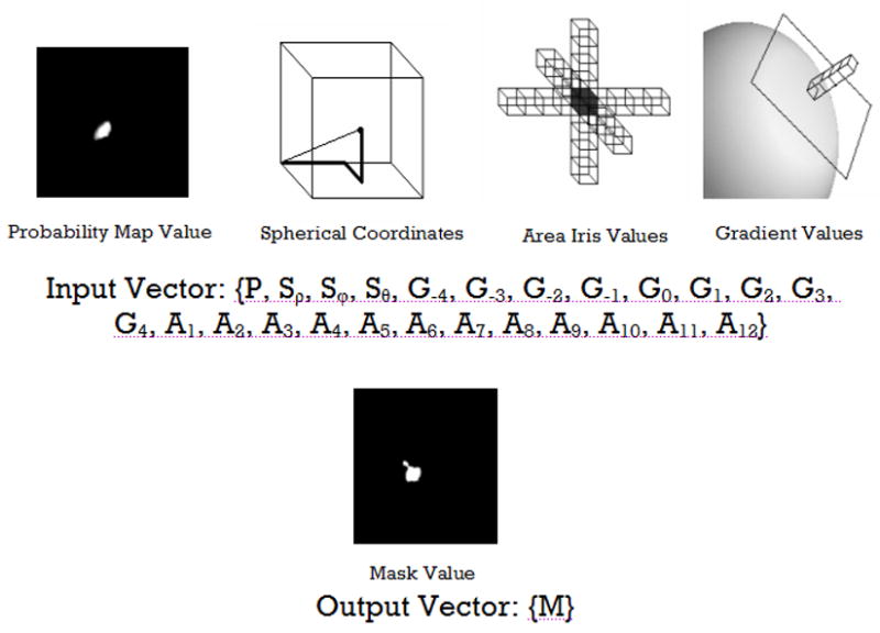
Training vector components. The training vectors include probability information, spherical coordinates, area iris values, signal intensity along the image gradient. The output of the neural network is a binary mask defining the region of interest.
2.5.2 Neural Network Training
Training was conducted using a learning rate of 0.30, a momentum term of 0.15, and a sigmoid activation function. The network was initialized by assigning random values for the weights connecting network nodes. The neural network was then applied to the training vectors and the mean square error was monitored to determine when the error reached an asymptote. Training was terminated at this point and the neural network weights were saved. It took approximately 250 iterations of the 500,000 input vectors to reach an asymptote. Training required approximately one day to complete. While this is a significant duration, it is completed only once per network configuration. Training was conducted for each structure separately, and the neural networks were trained to define a single structure within each network.
2.5.3 Application of the Neural Network
Once the neural network was trained, the neural network and resulting weights were applied to segment the structures on the reliability sample. The probability information was mapped to subject space using the same deformation fields created in the template based segmentation algorithm. The neural network model was then applied to the individual subjects and the resulting network activation function was filtered using a Gaussian filter of 0.5mm and thresholded at 0.5 to define the region of interest. Application of the neural network to the reliability sample took less than 5 minutes per subject.
2.6 Support Vector Machine Based Segmentation
The last segmentation algorithm investigated was a machine learning algorithm based on the support vector machine (SVM) architecture. The SVM algorithm used the same input vector information was the ANN algorithm. Conventional linear classifiers determine a single separating plane while SVM aims to calculate two planes of separation that maximize the margin of classification. The hyperplanes are described by the following set of equations:
| (1) |
and
| (2) |
where x ∈ RN and w is the normal of the hyperplane. The goal is to maximum the margin between the hyperplanes with no data points located between them. It can be shown that the distance between hyperplanes is 2/||w||, therefore the goal is to minimize ||w||. This results in a quadratic programming (QP) problem. The solution to this QP problem was generated using the optimization techniques described by Osuna et al (Osuna et al., 1997). While support vector machines were originally implemented to solve linear equations, they can be converted to solve non-linear problems by replacing the dot products in the above equations with a nonlinear kernel function. For this work a radial basis function was used.
Since QP techniques require a substantial amount of memory, a subset of 15,000 training vectors was arbitrarily chosen from the ANN training set. The decomposition algorithm was used to train the SVM. In this procedure, an initial subset of vectors was chosen and a solution for the subset was determined. Vectors not near the separating planes were replaced with unexamined vectors until all training vectors are examined. The SVM model comprised of these bounding support vectors was saved. SVM training was completed in approximately ten minutes per configuration. The SVM model was applied to segment the structures on the reliability sample. Application of the SVM based segmentation took approximately ten minutes per subject.
2.7 Reliability Evaluation of the Segmentation Algorithms
The reliability of the various segmentation algorithms were compared to the manually defined regions of interest from the reliability sample. To date there has been no consensus on the most appropriate metric to evaluate correspondence between segmented regions of interest; therefore the results reported in this paper are provided using three commonly used metrics: relative overlap, spatial overlap, and similarity index.
| (3) |
| (4) |
| (5) |
These three metric were chosen because they all compare spatial location, shape, and size between the two regions of interest. Intra-class correlations, another commonly used reliability metric, do not include shape or spatial location. Instead, intra-class correlations simply reflect the correspondence between the volumes.
2.7 Software
All software developed in this application was built upon the National Library of Medicine Insight Segmentation and Registration Toolkit (ITK), http://www.itk.org. This toolkit provided the framework for working with images and implementation of the image registration algorithms. The neural net code used the ANNIE Neural Network Library (http://annie.sourceforge.net/). LibSVM available at http://www.csie.ntu.edu.tw/~cjlin/libsvm/was incorporated for support of the SVM based image segmentation. The resulting programs are included with the BRAINS (Andreasen et al., 1992; Andreasen et al., 1993; Magnotta et al., 2002) image analysis software that is freely available from http://www.psychiatry.uiowa.edu/ipl.
3. RESULTS
The results for the four segmentation algorithms are shown in tables that report different reliability metrics: relative overlap (Table 2), similarity index (Table 3), and spatial overlap (Table 4). The template based segmentation algorithm had relative overlaps of 0.81, 0.80, and 0.84 for the caudate, putamen and thalamus respectively. The relative overlap for the hippocampus was lower at 0.59. The cerebellar regions have relative overlaps ranging from 0.70 to 0.83. The reliability metrics of similarity index and spatial overlap were higher for all structures. The probabilistic segmentation had very similar results as compared to the template based segmentation. This is true for all structures except the caudate where the template based segmentation had a higher relative overlap as shown in Table 5. The incorporation of machine learning into the segmentation algorithms significantly increased the relative overlap for all structures except the inferior posterior lobe of the cerebellum. ANN and SVM based segmentation did not differ significantly from each other. For all the segmentation algorithms the hippocampus had the lowest reliability. This held true for all of the reliability metrics. The SVM algorithm retained approximately 1000–2000 support vectors for each class after training.
Table 2.
Relative overlap (mean and standard deviation) of the four automated segmentation methods compared to a manual rater.
| Structure and Side | Template | Probability | ANN | SVM |
|---|---|---|---|---|
| Caudate
Left Right |
0.81 (0.04)
0.80 (0.03) 0.81 (0.04) |
0.77 (0.03)
0.76 (0.03) 0.77 (0.03) |
0.83 (0.04)
0.83 (0.04) 0.84 (0.04) |
0.84 (0.04)
0.84 (0.04) 0.84 (0.04) |
| Hippocampus
Left Right |
0.59 (0.02)
0.59 (0.05) 0.59 (0.08) |
0.62 (0.07)
0.63 (0.08) 0.62 (0.06) |
0.74 (0.04)
0.75 (0.03) 0.72 (0.04) |
0.72 (0.04)
0.74 (0.04) 0.71 (0.05) |
| Putamen
Left Right |
0.80 (0.03)
0.81 (0.04) 0.78 (0.03) |
0.80 (0.04)
0.80 (0.04) 0.79 (0.04) |
0.85 (0.03)
0.85 (0.03) 0.84 (0.02) |
0.84 (0.03)
0.84 (0.03) 0.83 (0.03) |
| Thalamus
Left Right |
0.84 (0.03)
0.84 (0.04) 0.84 (0.03) |
0.84 (0.03)
0.84 (0.03) 0.85 (0.02) |
0.88 (0.02)
0.88 (0.02) 0.88 (0.01) |
0.87 (0.03)
0.86 (0.03) 0.87 (0.02) |
| Anterior Lobe
Left Right |
0.70 (0.08)
0.72 (0.06) 0.69 (0.10) |
0.71 (0.07)
0.72 (0.06) 0.70 (0.08) |
0.77 (0.07)
0.78 (0.07) 0.77 (0.07) |
0.76 (0.06)
0.77 (0.05) 0.76 (0.06) |
| Corpus Medullare
Left Right |
0.78 (0.08)
0.81 (0.04) 0.76 (0.11) |
0.80 (0.08)
0.81 (0.05) 0.79 (0.11) |
0.85 (0.02)
0.85 (0.03) 0.84 (0.02) |
0.85 (0.03)
0.85 (0.03) 0.84 (0.03) |
| Inferior Posterior Lobe
Left Right |
0.83 (0.08)
0.84 (0.04) 0.82 (0.11) |
0.83 (0.08)
0.84 (0.06) 0.82 (0.11) |
0.87 (0.03)
0.86 (0.03) 0.88 (0.02) |
0.86 (0.03)
0.85 (0.03) 0.87 (0.02) |
| Superior Posterior Lobe
Left Right |
0.79 (0.07)
0.80 (0.04) 0.78 (0.09) |
0.79 (0.07)
0.79 (0.05) 0.79 (0.09) |
0.84 (0.03)
0.83 (0.04) 0.85 (0.03) |
0.83 (0.03)
0.83 (0.03) 0.84 (0.03) |
Table 3.
Similarity Index (mean and standard deviation) of the four automated segmentation methods compared to a manual rater.
| Structure and Side | Template | Probability | ANN | SVM |
|---|---|---|---|---|
| Caudate
Left Right |
0.89 (0.02)
0.89 (0.02) 0.89 (0.03) |
0.87 (0.02)
0.86 (0.02) 0.87 (0.02) |
0.91 (0.02)
0.91 (0.02) 0.91 (0.02) |
0.91 (0.02)
0.90 (0.02) 0.91 (0.02) |
| Hippocampus
Left Right |
0.74 (0.05)
0.74 (0.04) 0.74 (0.06) |
0.77 (0.05)
0.77 (0.06) 0.76 (0.05) |
0.85 (0.03)
0.86 (0.02) 0.84 (0.03) |
0.84 (0.03)
0.85 (0.02) 0.83 (0.03) |
| Putamen
Left Right |
0.89 (0.02)
0.90 (0.02) 0.88 (0.02) |
0.89 (0.02)
0.89 (0.02) 0.88 (0.03) |
0.92 (0.02)
0.92 (0.02) 0.92 (0.01) |
0.91 (0.02)
0.91 (0.02) 0.91 (0.02) |
| Thalamus
Left Right |
0.92 (0.02)
0.92 (0.02) 0.91 (0.02) |
0.91 (0.02)
0.91 (0.02) 0.92 (0.01) |
0.93 (0.01)
0.93 (0.01) 0.94 (0.01) |
0.93 (0.02)
0.93 (0.02) 0.93 (0.01) |
| Anterior Lobe
Left Right |
0.82 (0.06)
0.84 (0.04) 0.81 (0.07) |
0.83 (0.05)
0.84 (0.04) 0.82 (0.06) |
0.87 (0.04)
0.87 (0.04) 0.87 (0.05) |
0.86 (0.04)
0.87 (0.03) 0.86 (0.04) |
| Corpus Medullare
Left Right |
0.88 (0.06)
0.89 (0.02) 0.86 (0.08) |
0.89 (0.06)
0.90 (0.03) 0.88 (0.08) |
0.92 (0.01)
0.92 (0.01) 0.92 (0.01) |
0.92 (0.02)
0.92 (0.02) 0.91 (0.02) |
| Inferior Posterior Lobe
Left Right |
0.91 (0.06)
0.91 (0.03) 0.90 (0.08) |
0.90 (0.06)
0.91 (0.04) 0.90 (0.08) |
0.93 (0.02)
0.93 (0.02) 0.93 (0.01) |
0.92 (0.02)
0.92 (0.02) 0.93 (0.01) |
| Superior Posterior Lobe
Left Right |
0.88 (0.05)
0.89 (0.03) 0.87 (0.06) |
0.88 (0.05)
0.88 (0.03) 0.88 (0.06) |
0.91 (0.02)
0.90 (0.02) 0.92 (0.02) |
0.91 (0.02)
0.91 (0.02) 0.91 (0.02) |
Table 4.
Spatial Overlap (mean and standard deviation) of the four automated segmentation methods compared to a manual rater.
| Structure and Side | Template | Probability | ANN | SVM |
|---|---|---|---|---|
| Caudate
Left Right |
0.94 (0.04)
0.94 (0.04) 0.94 (0.04) |
0.82 (0.03)
0.82 (0.04) 0.82 (0.03) |
0.93 (0.03)
0.92 (0.04) 0.95 (0.03) |
0.91 (0.03)
0.90 (0.04) 0.92 (0.02) |
| Hippocampus
Left Right |
0.81 (0.08)
0.82 (0.07) 0.81 (0.10) |
0.73 (0.08)
0.73 (0.09) 0.74 (0.07) |
0.85 (0.04)
0.85 (0.04) 0.85 (0.05) |
0.82 (0.04)
0.83 (0.03) 0.82 (0.05) |
| Putamen
Left Right |
0.88 (0.03)
0.89 (0.03) 0.87 (0.04) |
0.84 (0.04)
0.84 (0.03) 0.84 (0.05) |
0.91 (0.03)
0.91 (0.03) 0.91 (0.03) |
0.90 (0.03)
0.89 (0.03) 0.89 (0.04) |
| Thalamus
Left Right |
0.92 (0.03)
0.92 (0.02) 0.93 (0.02) |
0.88 (0.02)
0.87 (0.02) 0.89 (0.02) |
0.93 (0.01)
0.93 (0.01) 0.93 (0.02) |
0.92 (0.02)
0.91 (0.02) 0.93 (0.02) |
| Anterior Lobe
Left Right |
0.84 (0.05)
0.83 (0.07) 0.86 (0.03) |
0.81 (0.05)
0.80 (0.06) 0.83 (0.04) |
0.88 (0.06)
0.84 (0.06) 0.91 (0.04) |
0.85 (0.05)
0.84 (0.06) 0.86 (0.04) |
| Corpus Medullare
Left Right |
0.89 (0.05)
0.91 (0.04) 0.87 (0.05) |
0.86 (0.05)
0.86 (0.05) 0.87 (0.06) |
0.92 (0.04)
0.92 (0.03) 0.92 (0.05) |
0.90 (0.05)
0.90 (0.05) 0.90 (0.05) |
| Inferior Posterior Lobe
Left Right |
0.92 (0.02)
0.93 (0.02) 0.91 (0.02) |
0.88 (0.03)
0.88 (0.03) 0.88 (0.03) |
0.90 (0.03)
0.90 (0.04) 0.90 (0.03) |
0.89 (0.03)
0.88 (0.03) 0.89 (0.02) |
| Superior Posterior Lobe
Left Right |
0.86 (0.03)
0.87 (0.04) 0.85 (0.03) |
0.83 (0.03)
0.83 (0.04) 0.83 (0.03) |
0.87 (0.04)
0.85 (0.05) 0.88 (0.03) |
0.86 (0.03)
0.86 (0.04) 0.86 (0.03) |
Table 5.
T-Test p-values of relative overlap measured between the segmentation methods.
| Structure | P-Values | |||||
|---|---|---|---|---|---|---|
| Template vs. Probabilistic | Template vs. ANN | Template vs. SVM | Probabilistic vs. ANN | Probabilistic vs. SVM | ANN vs. SVM | |
| Caudate | <0.01 | <0.01 | 0.03 | <0.01 | <0.01 | 0.34 |
| Hippocampus | 0.28 | <0.01 | <0.01 | <0.01 | <0.01 | 0.48 |
| Putamen | 0.98 | <0.01 | <0.01 | <0.01 | <0.01 | 0.16 |
| Thalamus | 0.79 | <0.01 | 0.02 | <0.01 | <0.01 | 0.18 |
| Anterior Lobe | 0.70 | <0.01 | <0.01 | 0.01 | 0.02 | 0.61 |
| Corpus Medullare | 0.47 | <0.01 | <0.01 | 0.03 | 0.04 | 0.83 |
| Inferior Posterior Lobe | 0.95 | 0.05 | 0.13 | 0.04 | 0.13 | 0.26 |
| Superior Posterior Lobe | 0.94 | <0.01 | <0.01 | <0.01 | <0.01 | 0.78 |
The relative overlap of the template based segmentation method was comparable to the manual rater reliability for the caudate, putamen, and thalamus. Structures such as the hippocampus and cerebellar regions had significantly lower reliability as compared to the manual raters. Employing machine learning algorithms resulted in relative overlap measures that were comparable to the manual raters on all regions except for the anterior lobe of the cerebellum. The only difference in the atlas based segmentations (single template versus probabilistic template) was found in the caudate where the single template outperformed the probabilistic template. The machine learning algorithms contain additional anatomical information including spatial position and information about the signal intensity in the surrounding voxels. This information helps the machine learning algorithms to identify the boundaries in regions where anatomical boundaries are fuzzy and greater residual anatomic variability remains. This is evident in structures such as the hippocampus and cerebellum.
A visual comparison of the automated methods to the manual rater is shown in Figure 2 for the subcortical regions, Figure 3 for the hippocampus and Figure 4 for the cerebellum. In all cases the manual definition is in red. The automated definitions are shown in blue in Figures 2–3. In Figure 4, a different color is used to define each of the automated segmentation regions of interest. All of the automated segmentation algorithms tend to follow the border defined by a manual rater very closely. The template based segmentation tended to have the largest deviation from the manually defined border. This is clear in the Figure 2 for the putamen and Figure 3 showing the hippocampus. Figure 5 shows a surface representation for the ANN segmented regions of interest from a subject in the testing set. The cortical surface is shown for reference.
Figure 2.
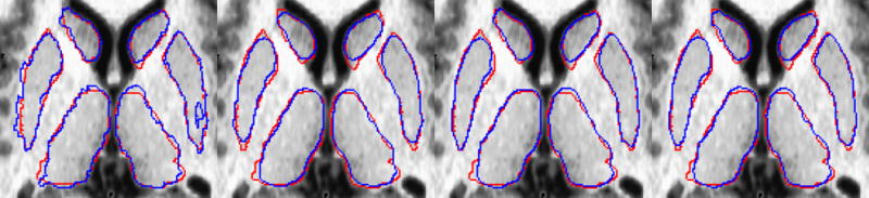
Manual (red) and automated (blue) defined regions of interest are shown for the caudate, putamen, and thalamus. The template, probabilistic, ANN, and SVM automated segmentations are shown from left to right.
Figure 3.
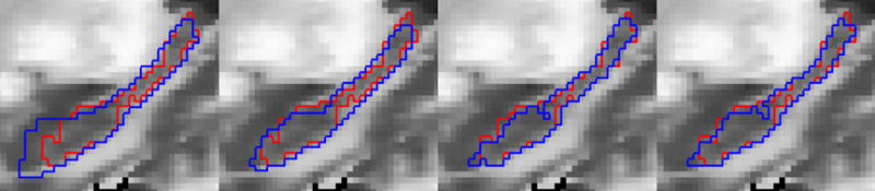
Manual (red) and automated (blue) defined regions of interest are shown for the hippocampus. The template, probabilistic, ANN, and SVM automated segmentations are shown from left to right.
Figure 4.
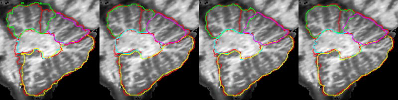
Manual (red) and automated defined regions of interest are shown for the cerebellum. The automated regions are shown in green (anterior), pink (superior posterior), yellow (inferior posterior), and light-blue (corpus medullare). The template, probabilistic, ANN, and SVM automated segmentations are shown from left to right.
Figure 5.
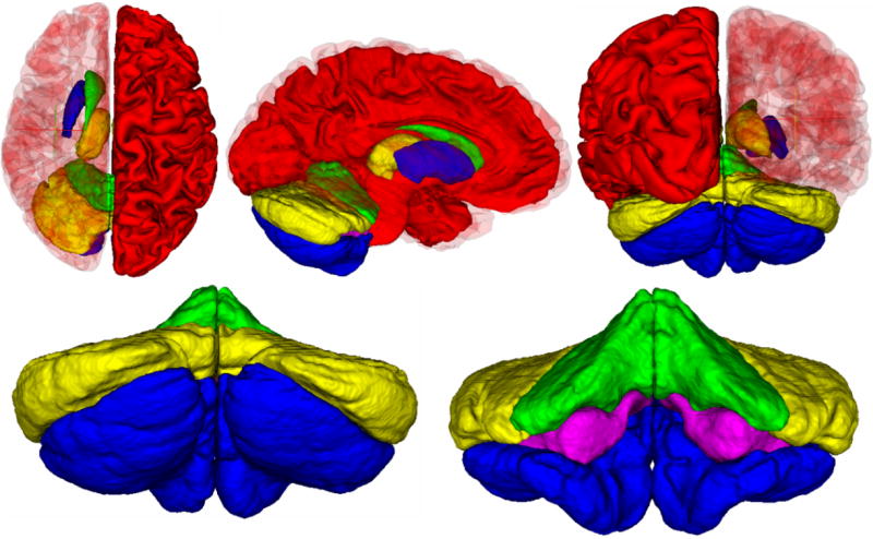
Surface definitions of the ANN automatically defined regions of interest (excluding the cortical surface). For the subcrotical regions, the caudate is shown in green, putamen in blue, and thalamus in yellow. The cerebellar regions include the corpus medullare (pink), anterior (green), superior posterior (blue), and inferior posterior (yellow) lobes.
The results show that the relative overlap metric has the greatest penalty for shape differences between the automated segmentation and the manual rater. This is due to the dominator of the metric. The volume of the union for the two regions is guaranteed to be greater than or equal to the volume of the manual rater or the average volume of the two regions. Spatial overlap imposes the smallest shape penalty. In fact, spatial overlap will produce its maximum value of 1 for any generated region that fully encompasses the entire manually defined region.
4. DISCUSSION
Atlas, probability, ANN, and SVM based automated segmentation methods have been developed to automatically delineate subcortical and cerebellar regions of interest. Relative overlap of the subcortical and cerebellar structures by the template based method ranged from 0.59 to 0.84. The hippocampus had the lowest relative overlap at 0.59. This is similar to the results obtained by Wu et al. (Wu et al. 2006) who obtained relative overlap of 0.62 using a similar technique. The probabilistic atlas approach had similar results as compared to the template method. Relative overlaps ranged from 0.62 to 0.84 for the structures utilized in this study. Improvements in the resulting relative overlaps came from the application of the machine learning methods including ANN and SVM. The relative overlap ranged from 0.74 to 0.88 for the ANN based methods and from 0.74 to 0.87 for the support vector machine algorithm. The previous utilization of the ANN method by Magnotta et al. (Magnotta et al. 1999) resulted in relative overlap measures of 0.80, 0.76, and 0.83 for the caudate, putamen, and thalamus respectively. Similar results were obtained in this work using the template based segmentation. With the modifications to the ANN input vector information the relative overlaps increased to 0.84, 0.84, and 0.87 for these same regions. In this implementation, the SVM parameter space was not fully explored. Future work could be undertaken to explore weighting of certain features (e.g. probability and signal intensity) greater than others (e.g. spatial position).
A comparison between the four methods shows that the machine learning algorithms outperform the template and probabilistic based methods when examining the relative overlap (Table 5). This metric was used because it is the most sensitive to shape differences. The relative overlap between the manual raters ranged from 0.72 to 0.86 for the subcortical and cerebellar structures. The machine learning algorithms were as reliable as manual segmentation based on the relative overlap values, and can be applied to large datasets in a small fraction of the time required by manual raters. Rater drift is also eliminated using these automated approaches to image segmentation.
To compare the automated segmentation methods with previously published methods, similarity index and spatial overlap were examined. Spatial overlap measurements were similar for all of the applied methods and ranged from 0.84 to 0.94 across all methods and structures. The spatial overlap measured by Iosifescu et al. (1997) was 0.78, 0.78, and 0.85 for the caudate, putamen, and thalamus respectively. The ANN algorithm provided spatial overlap of 0.93, 0.91, and 0.93 for the same structures. Fischl et al. (2002) reported similarity indices ranging from 0.80 to 0.88 for the subcortical structures. However, the data presented by Fischl et al. relied on only the use of T1 weighted images while the methods presented here utilized data from a multi-modal imaging protocol.
This work provides a direct comparison between four automated segmentation methods using the same data set. The machine learning algorithms outperformed the template and probabilistic based segmentation methods, suggesting that the inclusion of additional information such as surrounding voxel signal intensity can improve segmentation performance. There is also little disparity between the ANN and SVM based segmentation algorithms. ANN training takes significantly longer than SVM training, but can be applied more quickly to segment the regions of interest. An expert manual rater who reviewed the results could not differentiate between the manually and machine learning defined regions of interest. The neural network and support vector machine models produced by this algorithm may be utilized to accurately delineate subcortical and cerebellar regions of interest in a matter of minutes.
The advantage of the proposed machine learning algorithms is the ability to define anatomic regions of interest with a high degree of reliability in regions where the anatomy is fairly homogenous. The algorithms may not generalize to defining cortical regions of interest due to the greater degree of heterogeneity. For this region, unsupervised algorithms may have a distinct advantage.
As the number of multi-center studies grows, there is increased demand for development and utilization of methods that can automate the segmentation of cortical, subcortical and cerebellar regions of interest. These methods in addition to be being automated need to identify subtle brain changes. The artificial intelligence based methods presented in this paper have reliability similar to a human rater across a variety of structures. By using a completely automated segmentation process, the possibility of rater drift is eliminated if the same model is applied throughout a longitudinal study. Additionally, application of an automated process reduces rater bias by minimizing human interaction in the decision making process for delineation of structures. The algorithms presented here are appropriate for large scale imaging studies.
Footnotes
Publisher's Disclaimer: This is a PDF file of an unedited manuscript that has been accepted for publication. As a service to our customers we are providing this early version of the manuscript. The manuscript will undergo copyediting, typesetting, and review of the resulting proof before it is published in its final citable form. Please note that during the production process errors may be discovered which could affect the content, and all legal disclaimers that apply to the journal pertain.
References
- Acosta MT, Pearl PL. Imaging data in autism: from structure to malfunction. Semin Pediatr Neurol. 2004;11(3):205–13. doi: 10.1016/j.spen.2004.07.004. [DOI] [PubMed] [Google Scholar]
- Akselrod-Ballin A, Galun M, Gomori MJ, Basri R, Brandt A. Atlas guided identification of brain structures by combining 3D segmentation and SVM classification. Med Image Comput Comput Assist Interv Int Conf Med Image Comput Comput Assist Interv. 2006;9:209–16. doi: 10.1007/11866763_26. [DOI] [PubMed] [Google Scholar]
- Andreasen NC, Cizadlo T, Harris G, Swayze V, 2nd, O’Leary DS, Cohen G, Ehrhardt J, Yuh WT. Voxel processing techniques for the antemortem study of neuroanatomy and neuropathology using magnetic resonance imaging. J Neuropsychiatry Clin Neurosci. 1993;5(2):121–30. doi: 10.1176/jnp.5.2.121. [DOI] [PubMed] [Google Scholar]
- Andreasen NC, Cohen G, Harris T, Cizadlo T, Parkkinen J, Rezai K, Swayze VW., 2nd Image processing for the study of brain structure and function: problems and programs. J Neuropsychiatry Clin Neurosci. 1992;4(2):125–33. doi: 10.1176/jnp.4.2.125. [DOI] [PubMed] [Google Scholar]
- Ashburner JA, Sndreson JL, Friston KJ. Image registration using a symmetric prior—in three dimensions. Human Brain Mapping. 1999;9:212–25. doi: 10.1002/(SICI)1097-0193(200004)9:4<212::AID-HBM3>3.0.CO;2-#. [DOI] [PMC free article] [PubMed] [Google Scholar]
- Bookstein FL. Thin-plate splines and the atlas problem for biomedical images. Int Conf Information Processing in Medical Imaging. 1991;12:326–342. [Google Scholar]
- Cagnoni S, Coppini G, Rucci M, Caramella D, Valli G. Neural network segmentation of magnetic resonance spin echo images of the brain. J Biomed Eng. 1993;15(5):355–62. doi: 10.1016/0141-5425(93)90071-6. [DOI] [PubMed] [Google Scholar]
- Clarke LP, Velthuizen RP, Phuphanich S, Schellenberg JD, Arrington JA, Silbiger M. MRI: stability of three supervised segmentation techniques. Magn Reson Imaging. 1993;1993;11(1):95–106. doi: 10.1016/0730-725x(93)90417-c. [DOI] [PubMed] [Google Scholar]
- Dickson S, Thomas BT, Goddard P. Using neural networks to automatically detect brain tumours in MR images. Int J Neural Syst. 1997;8(1):91–9. doi: 10.1142/s0129065797000124. [DOI] [PubMed] [Google Scholar]
- Fischl B, Salat DH, Busa E, Albert M, Dieterich M, Haselgrove C, van der Kouwe A, Killiany R, Kennedy D, Klaveness S, Montillo A, Makris N, Rosen B, Dale AM. Whole brain segmentation: automated labeling of neuroanatomical structures in the human brain. Neuron. 2002;33(3):341–55. doi: 10.1016/s0896-6273(02)00569-x. [DOI] [PubMed] [Google Scholar]
- Glass JO, Ji Q, Glas LS, Reddick WE. Prediction of total cerebral tissue volumes in normal appearing brain from sub-sampled segmentation volumes. Magn Reson Imaging. 2003;21(9):977–82. doi: 10.1016/j.mri.2003.05.010. [DOI] [PubMed] [Google Scholar]
- Grevera GJ, Udupa JK. Shape-based interpolation of multidimensional grey-level images. IEEE Trans Med Imaging. 1996;15:881–892. doi: 10.1109/42.544506. [DOI] [PubMed] [Google Scholar]
- Harris G, Andreasen NC, Cizadlo T, Bailey JM, Bockholt HJ, Magnotta VA, Arndt S. Improving tissue classification in MRI: a three-dimensional multispectral discriminant analysis method with automated training class selection. J Comput Assist Tomogr. 1999;23(1):144–54. doi: 10.1097/00004728-199901000-00030. [DOI] [PubMed] [Google Scholar]
- Hellier P, Ashburner J, Corouge I, Barillot C, Friston KJ. Inter-subject registration of functional and anatomical data using SPM. 5th International Conference on Medical Image Computing and Computer-Assisted Intervention MICCAI’2002, Lecture Notes in Computer Science, Vol. 2489; Tokyo, Japan. September 2002; 2002. pp. 590–597. [Google Scholar]
- Holmes CJ, Hoge R, Collins L, Woods R, Toga AW, Evans AC. Enhancement of MR images using registration for signal averaging. J Comput Assist Tomogr. 1998;22:324–333. doi: 10.1097/00004728-199803000-00032. [DOI] [PubMed] [Google Scholar]
- Iosifescu DV, Shenton ME, Warfield SK, Kikinis R, Dengler J, Jolesz FA, McCarley RW. An automated registration algorithm for measuring MRI subcortical brain structures. Neuroimage. 1997;6(1):13–25. doi: 10.1006/nimg.1997.0274. [DOI] [PubMed] [Google Scholar]
- Lin JS, Cheng KS, Mao CW. Multispectral magnetic resonance images segmentation using fuzzy Hopfield neural network. Int J Biomed Comput. 1996;42(3):205–14. doi: 10.1016/0020-7101(96)01199-3. [DOI] [PubMed] [Google Scholar]
- Lin JS, Cheng KS, Mao CW. Segmentation of multispectral magnetic resonance image using penalized fuzzy competitive learning network. Comput Biomed Res. 1996;29(4):314–26. doi: 10.1006/cbmr.1996.0023. [DOI] [PubMed] [Google Scholar]
- Magnotta VA, Harris G, Andreasen NC, O’Leary DS, Yuh WT, Heckel D. Structural MR image processing using the BRAINS2 toolbox. Comput Med Imaging Graph. 2002;26(4):251–64. doi: 10.1016/s0895-6111(02)00011-3. [DOI] [PubMed] [Google Scholar]
- Magnotta VA, Heckel D, Andreasen NC, Cizadlo T, Corson PW, Ehrhardt JC, Yuh WT. Measurement of brain structures with artificial neural networks: two- and three-dimensional applications. Radiology. 1999;211(3):781–90. doi: 10.1148/radiology.211.3.r99ma07781. [DOI] [PubMed] [Google Scholar]
- Mulhern RK, Reddick WE, Palmer SL, Glass JO, Elkin TD, Kun LE, Taylor J, Langston J, Gajjar A. Neurocognitive deficits in medulloblastoma survivors and white matter loss. Ann Neurol. 1999;46(6):834–41. doi: 10.1002/1531-8249(199912)46:6<834::aid-ana5>3.0.co;2-m. [DOI] [PubMed] [Google Scholar]
- Osuna EE, Freund R, Girosi F. AI Memo, MIT AI Lab. 1996. Support Vector Machines: Training and Applications. [Google Scholar]
- Pantel J, O’Leary DS, Cretsinger K, Bockholt HJ, Keefe H, Magnotta VA, Andreasen NC. A new method for the in vivo volumetric measurement of the human hippocampus with high neuroanatomical accuracy. Hippocampus. 2000;10(6):752–8. doi: 10.1002/1098-1063(2000)10:6<752::AID-HIPO1012>3.0.CO;2-Y. [DOI] [PubMed] [Google Scholar]
- Perez de Alejo R, Ruiz-Cabello J, Cortijo M, Rodriguez I, Echave I, Regadera J, Arrazola J, Aviles P, Barreiro P, Gargallo D, Grana M. Computer-assisted enhanced volumetric segmentation magnetic resonance imaging data using a mixture of artificial neural networks. Magn Reson Imaging. 2003;21(8):901–12. doi: 10.1016/s0730-725x(03)00193-0. [DOI] [PubMed] [Google Scholar]
- Pierson R, Corson PW, Sears LL, Alicata D, Magnotta V, Oleary D, Andreasen NC. Manual and semiautomated measurement of cerebellar subregions on MR images. Neuroimage. 2002;17(1):61–76. doi: 10.1006/nimg.2002.1207. [DOI] [PubMed] [Google Scholar]
- Piraino DW, Amartur SC, Richmond BJ, Schils JP, Thome JM, Weber PB. Segmentation of magnetic resonance images using an artificial neural network. Proc Annu Symp Comput Appl Med Care. 1991:470–2. [PMC free article] [PubMed] [Google Scholar]
- Prakash B, Gupta V, Bilello M, Beauchamp NJ, Nowinski NL. Identification, Segmentation, and image property study of acute infarcts in Diffusion-Weighted images by using a probabilistic neural network and adaptive Gaussian mixture model. Acad Radiol. 2006;13:1474–1484. doi: 10.1016/j.acra.2006.09.045. [DOI] [PubMed] [Google Scholar]
- Reddick WE, Glass JO, Cook EN, Elkin TD, Deaton RJ. Automated segmentation and classification of multispectral magnetic resonance images of brain using artificial neural networks. IEEE Trans Med Imaging. 1997;16(6):911–8. doi: 10.1109/42.650887. [DOI] [PubMed] [Google Scholar]
- Shen S, Sandham W, Granat M, Sterr A. MRI fuzzy segmentation of brain tissue using neighborhood attraction with neural-network optimization. IEEE Trans Inf Technol Biomed. 2005;9(3):459–67. doi: 10.1109/titb.2005.847500. [DOI] [PubMed] [Google Scholar]
- Song T, Gasparovic C, Andreasen N, Bockholt J, Jamshidi M, Lee RR, Huang M. A hybrid tissue segmentation approach for brain MR images. Med Biol Eng Comput. 2006;44(3):242–9. doi: 10.1007/s11517-005-0021-1. [DOI] [PubMed] [Google Scholar]
- Spinks R, Magnotta VA, Andreasen NC, Albright KC, Ziebell S, Nopoulos P, Cassell M. Manual and automated measurement of the whole thalamus and mediodorsal nucleus using magnetic resonance imaging. Neuroimage. 2002;17(2):631–42. [PubMed] [Google Scholar]
- Strzelecki M, Materka A, Drozdz J, Krzeminska-Pakula M, Kasprzak JD. Classification and segmentation of intracardiac masses in cardiac tumor echocardiograms. Computerized Medical Imaging and Graphics. 2006;30:95–107. doi: 10.1016/j.compmedimag.2005.11.004. [DOI] [PubMed] [Google Scholar]
- Talairach J, Tournoux P. Co-planar stereotaxic atlas of the human brain. Thieme; Stuttgart, Germany: 1988. [Google Scholar]
- Thirion JP. Image matching as a diffusion process: an analogy with Maxwell’s demons. Med Image Anal. 1998;2(3):243–60. doi: 10.1016/s1361-8415(98)80022-4. [DOI] [PubMed] [Google Scholar]
- Valdes-Cristerna R, Medina-Banuelos V, Yanez-Suarez O. Coupling of radial-basis network and active contour model for multispectral brain MRI segmentation. IEEE Trans Biomed Eng. 2004;51(3):459–70. doi: 10.1109/TBME.2003.820377. [DOI] [PubMed] [Google Scholar]
- Wagenknecht G, Kaiser HJ, Buell U, Sabri O. MRI-based individual 3D region-of-interest atlases of the human brain: a new method for analyzing functional data. Methods Inf Med. 2004;43(4):383–90. [PubMed] [Google Scholar]
- Wismuller A, Vietze F, Behrends J, Meyer-Baese A, Reiser M, Ritter H. Fully automated biomedical image segmentation by self-organized model adaptation. IEEE Trans Med Imaging. 2006;25(1):62–73. doi: 10.1016/j.neunet.2004.06.015. [DOI] [PubMed] [Google Scholar]
- Woods RP, Grafton ST, Holmes CJ, Cherry SR, Mazziotta JC. Automated image registration: II. Intersubject validation of linear and nonlinear models. J Comput Assist Tomogr. 1998;22(1):153–65. doi: 10.1097/00004728-199801000-00028. [DOI] [PubMed] [Google Scholar]
- Wu M, Carmichael O, Lopez-Garcia P, Carter CS, Aizenstein HJ. Quantitative comparison of AIR, SPM, and the fully deformable model for atlas-based segmentation of functional and structural MR images. Hum Brain Mapp. 2006 doi: 10.1002/hbm.20216. Published Online: 6 Feb 2006. [DOI] [PMC free article] [PubMed] [Google Scholar]