

Abstract
MRI-based study of 3He gas diffusion in lungs may provide important information on lung microstructure. Lung acinar airways can be described in terms of cylinders covered with alveolar sleeve (Haefeli-Bleuer, Weibel, Anat. Rec., 1988, 220, 401). For relatively short diffusion times (on the order of a few ms) this geometry allows description of the 3He diffusion attenuated MR signal in lungs in terms of two diffusion coefficients - longitudinal (DL) and transverse (DT) with respect to the individual acinar airway axis (Yablonskiy et al, PNAS, 2002, 99, 3111). In this paper, empirical relationships between DL and DT and the geometrical parameters of airways and alveoli are found by means of computer Monte Carlo simulations. The effects of non-Gaussian signal behavior (dependence of DL and DT on b-value) are also taken into account. The results obtained are quantitatively valid in the physiologically important range of airway parameters characteristic of healthy lungs and lungs with mild emphysema. In lungs with advanced emphysema, the results provide only “apparent” characteristics but still could potentially be used to evaluate emphysema progression. This creates a basis for in vivo lung morphometry - evaluation of the geometrical parameters of acinar airways from hyperpolarized 3He diffusion MRI, despite the airways being too small to be resolved by direct imaging. These results also predict a rather substantial dependence of 3He ADC on the experimentally-controllable diffusion time, Δ. If Δ is decreased from 3 ms to 1 ms, the ADC in normal human lungs may increase by almost 50%. This effect should be taken into account when comparing experimental data obtained with different pulse sequences.
Keywords: diffusion MRI, hyperpolarized gas, lung airways, apparent diffusion coefficient
Introduction
Hyperpolarized 3He gas and some other hyperpolarized gases are now broadly used in MRI as inhaled contrast agents for investigating lung structure and functioning. One of the directions in these investigations relies on studying 3He gas diffusion in lungs. As diffusion in lungs, especially, at the acinar level, is strongly restricted by alveoli, it might provide important insights on lung microstructure. To make this information quantitative, relationships between lung microstructure parameters and a diffusion attenuated MR signal are required. One of the approaches - in vivo lung morphometry technique [1] - is based on a well known geometrical model of the lung, in which acinar lung airways are considered as cylinders covered by alveolar sleeves [2]. Accordingly, in [1] diffusion of 3He gas in each airway is considered to be anisotropic and described by distinct longitudinal and transverse diffusion coefficients, DL and DT. Then, in each airway a MR signal with respect to b-value was assumed as:
| (1) |
where S0 is the MR signal intensity in the absence of diffusion-sensitizing gradients, α is the angle between the diffusion gradient and the cylinder’s axis, and the b-value is determined by the gradient waveform shape, strength, and timing. With the spatial resolution of several millimeters currently available with 3He MRI, each voxel contains hundreds of acinar airways with different orientations. Under a reasonable assumption of a uniform distribution of airway orientations, the total MR signal from a voxel is [1]:
| (2) |
where Φ(x) is the error function and DAN = DL - DT is the diffusion anisotropy. This macroscopically isotropic but microscopically anisotropic model allows the estimation of these diffusion coefficients from multi b-value MR measurements [1].
While some computer simulations of 3He gas diffusion in alveolar ducts [3, 4] demonstrated a rather good agreement with the results of the model [1], no systematic study of the relationship between airway geometrical parameters and model parameters (DL and DT) has been conducted. This is a major subject of the current paper. Also in this paper we expand the theoretical model [1] by incorporating the effects of non-Gaussian signal behavior (i.e. the dependence of DL and DT on b-value). We focus our attention on diffusion at times Δ of several milliseconds, which is a typical diffusion time used in most experiments (see, e.g., [1, 4-28]). Here a diffusing 3He atom samples a distance smaller than the acinar airway length but comparable with the airway radius. From a theoretical perspective, this diffusion time belongs to an intermediate regime where developing an analytical theory faces substantial difficulties. Thus, the problem is studied herein by means of computer Monte Carlo simulations.
Simulations uncovered remarkable scaling relationships between diffusion coefficients and lung geometrical parameters. This allowed presenting results in a rather compact form:
| (3) |
where
| (4) |
Here D0 is the free diffusion coefficient of 3He gas in lung airspaces; and are the characteristic free-diffusion lengths for one- and two-dimensional diffusion, respectively; R and r are the external and internal airway radii, L is the alveolar size, as defined below in Fig. 1. With an average accuracy of about 1-3%, Eqs. (3)-(4) are valid within the intervals and r / R > 0.4. For typical diffusion time Δ = 1.8ms, is 563 μm, so that R must be less than 400 μm. This interval covers not only typical radii of acinar alveolar ducts in healthy human lungs but those in small animals (e.g., mice, rats) as well.
Fig. 1.
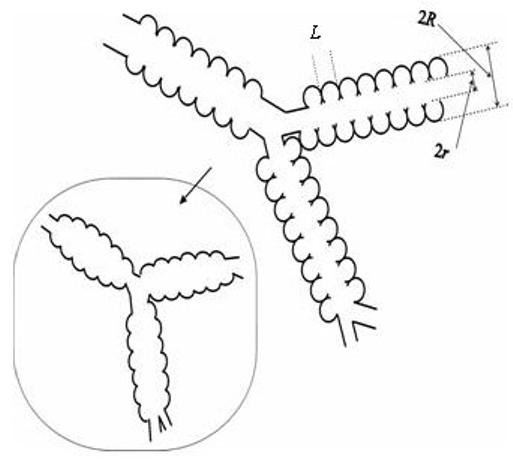
Schematic structure of two levels of acinar airways. Open spheres represent alveoli forming an alveolar sleeve around each airway. Inset schematically represents the structure of the same airways in emphysema, scaled down for clarity.
Applying Eqs. (2-4) to multi-b measurements of the 3He diffusion attenuated MRI signal in lung airways makes possible the in vivo evaluation of mean geometrical parameters of lung acinar airways, in spite of the airways being too small to be resolved by direct imaging. MRI-based measurement of airways parameters in healthy and emphysematous lungs may provide an important non-invasive tool for identifying changes in lung structure at the alveolar level.
Methods
Geometrical model
According to the lung geometrical model [2] adopted in [1], acinar airways are considered as cylinders covered by sleeves formed by alveoli (open spheres in Fig. 1). The diagram defines inner (r) and outer (R) radii (as in Fig. 1 in [2]) and the distance between alveolar walls, L (this parameter can also be considered as a mean alveoli size). In humans, depending on the branching level of the acinar airway tree, the internal acinar airway radius r varies in the interval from 135 μm to 250 μm, whereas the outer radius R (including the sleeve of alveoli) remains practically constant at 350 μm [2]. 93% of the gas is in the acinar units, so restricting our simulations to acinar airways is a good approximation.
In the computer simulations below, we mimic an acinar airway by a periodic structure of cylindrical symmetry; one segment of the structure is shown in Fig. 2 (one of four alveoli is removed). The alveolar walls are considered impermeable to the gas atoms. A similar model of the alveolar duct was used for numerical solution of the diffusion equation in [29]; however, in our model as well as in the model used in [3], each alveolus covers ¼ of an annular ring rather than ⅛ in [29]; we will demonstrate below that in the physiological range of r / R this difference is not important for diffusion calculations.
Fig. 2.
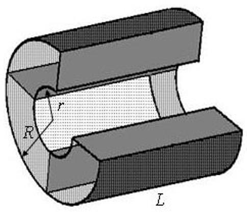
Model of acinar airway covered by alveolar sleeve (alveolar duct) corresponding to the structure depicted in Fig. 1. One segment of the periodic structure is shown; one of four alveoli is removed.
Our model of acinar airway is described by three geometrical parameters - external radius, R, internal radius, r, and the distance between alveolar walls, L. The intervals over which these parameters vary were chosen in the physiological range characteristic for healthy or slightly emphysematous human lungs or lungs of large animals. However, the scaling relationships that we found allow the application of the derived expressions to small animals as well. For Monte-Carlo simulations we vary R in the interval 300-400 μm. The distance L, according to preliminary estimates, does not deviate from R more than 20%, therefore the simulations are performed in the range 0.8 < L / R < 1.2. Although the simulations were performed in the whole range of possible r (0 < r < R), attention is paid primarily to the physiological range r / R > 0.4 .
Computer simulations
Computer simulations of random-walks were performed on M independent particles with random starting positions, with M typically 106-107. At each computer step of duration Δt, a particle moves with equal probability in one of 8 directions (±1, ±1, ±1) over distance l0 = (6D0 · Δt)1/2, where D0 = 0.88 cm2 /s is the free diffusion coefficient of 3He gas in N2 or air. The time step was chosen to ensure that the distance l0 is much smaller than any sizes of the geometrical model.
At each step j of a random walk through a magnetic field gradient, a particle gains a phase
| (5) |
where γ is the gyromagnetic ratio, r(tj) is he position of the particle at step j, and G(tj) is the time-dependent magnetic field gradient introduced as usual for diffusion encoding. The index j enumerates computer time steps running from 0 to N = T / Δt, where T is the full sequence time and tj = j · Δt. If a contemplated jump would pass through any boundary (see Fig. 2), the move was rejected and the particle remained at the initial position. For our simulations, we use Δt = 1 μs, corresponding to the jump distance l0 = 23 μm. We have verified that using simulations with random step directions (rather than eight), and/or more complicated reflection laws, and/or shorter Δt does not affect the result of simulations; however, the use of these methods leads to longer computational times and were therefore not used.
The MR signal, S, was calculated by averaging signals from M individual particles:
| (6) |
The Monte Carlo algorithm was thoroughly tested to ensure its proper functioning by comparing the MR signal obtained by simulations with the exact analytical (or close-to-analytical) results known for simple geometries (one-dimensional interval, circle and sphere) [30, 31]. The results of these simulations demonstrate excellent agreement with analytical predictions.
In most simulations, we use a diffusion sensitizing gradient waveform (see Fig. 3) with parameters similar to those in [1] and typical for human imaging: diffusion time Δ = δ = 1.8 ms, gradient ramp time τ = 0.3 ms. However, as it will be demonstrated below, the results are valid for a rather broad range of diffusion parameters Δ, δ, and τ. The b-value corresponding to such a pulse sequence is equal to [1, 32]:
| (7) |
where Gm is the gradient amplitude. The simulations were performed for different orientations of the gradient with respect to the cylinder’s axis and different gradient amplitudes Gm; the b-dependent apparent diffusion coefficient D(α,b) was calculated as:
| (8) |
In particular, if the gradient G is parallel to the cylinder’s axis, D(0,b) = DL; for G oriented perpendicular to the cylinder axis, D(π / 2,b) = DT. In what follows, the sequence timing parameters are kept constant and the b-value is altered from 0 to 10 s/cm2 by changing the gradient amplitude Gm.
Fig. 3.

Diffusion sensitizing pulse gradient waveform employed in simulations.
Results
Longitudinal diffusivity
To analyze the longitudinal diffusivity DL, the simulations were performed with the gradient G(t) parallel to the cylinder axis. Obviously, in the case of smooth cylinders, diffusion in this direction would be free, and DL = D0. The internal boundaries depicted in Fig. 2 impede longitudinal diffusion, with a smaller internal radius r resulting in more restricted diffusion and a smaller longitudinal diffusivity DL.
Figure 4 illustrates the dependence of DL on the b-value for different internal radii r. In the simulations shown below, we use R = L = 350μm which corresponds to a typical alveolar duct size in healthy lungs. In the case r = R corresponding to free diffusion in the direction parallel to the cylinder’s axis, DL = D0 and does not depend on the b-value, as expected. For all other values of r < R, diffusion is restricted and DL depends on b. In the most interesting physiological range of r (150-200 μm), the slope reaches its maximum; for instance, for r = 150 μm the longitudinal diffusivity DL changes from 0.35 cm2/s at b = 0.5 s/cm2 to 0.25 cm2/s at b =10 s/cm2 (30% decrease).
Fig. 4.

The longitudinal diffusivity DL as a function of the b-value for different internal radii r (shown by numbers near the lines; in μm). Symbols represent the results of simulations; straight lines - linear fit to Eq. (9). R=L=350μm, Δ = 1.8 ms, τ = 0.3 ms. Data are truncated for bDL > 2, corresponding to the MR signal decay of e-2.
This b-dependence of DL can be well approximated by a linear function,
| (9) |
the coefficients DL0 and βL being found by fitting Eq. (9) to the data for DL (b) by means of a standard Levenberg-Markquart algorithm. The same algorithm was used for fitting procedures all over the study. The sign “-” in Eq. (9) is chosen for convenience because the slope of the functions DL (b) is positive only for the line corresponding r = 0 (completely closed cylinder) and negative for all the other lines shown in Fig. 4. Note that the coefficient βL (and a similar coefficient βT in the transverse diffusivity, see Eq. (16) below) reflects non-Gaussian diffusion effects in each individual airway and is proportional to the so called kurtosis K - the second order term in the cumulant expansion of the MR signal (e.g., [33-35]); (KL = 6βL, KT = -6βT). It should be emphasized, however, that the original model for the signal S(b) in Eq. (2) also demonstrated non-monoexponentiality in b-value, which was due to orientation averaging of the signals from individual airways S(b; α), Eq. (1). The non-monoexponentiality in b-value described by coefficients βL and βT for individual orientations and thus is in addition to this “averaging” effect.
To analyze the dependence of the phenomenological parameters DL0 and βL on airway geometrical characteristics, we note that the system under consideration is characterized by four parameters of length: R, L, r, and the characteristic diffusion distance ( for Δ = 1.8 ms used in our simulation). Therefore, the parameters DL0 and βL in Eq. (9) may depend, generally, on three dimensionless ratios: r / R, L / R and . Figure 5 illustrates the dependences of DL0 and βL on the dimensionless parameter r / R for R = 350 μm and different L (300, 350, and 400 μm). The parameter DL0 monotonically increases from small values at r = 0 and tends to the free diffusion coefficient D0 = 0.88 cm2/s at r / R → 1. The parameter βL rapidly increases from small negative values at r = 0, reaching its maxima at r / R ∼ 0.2 and then monotonically decreasing to 0 at r / R → 1. Such behavior of the parameter βL should be expected because at r = 0 the airway is completely closed and longitudinal diffusion is strongly restricted by the alveolar walls separated by the distance L, which is smaller than the diffusion distance . In this limit, diffusion can be approximately described by the Gaussian phase approximation, where the signal is close to monoexponential with respect to b-value (for fixed Δ). In the opposite limit r / R → 1 diffusion becomes free and once again the signal behavior is monoexponential with b. In both these case βL tends to zero, as in Fig. 5b.
Fig. 5.


The parameters DL0 (a) and βL (b) as functions of r / R for R = 350 μm and different L.
Simulations with different external radii R and distances L (R=300 μm and L=250-350 μm; R=350 μm and L=300-400 μm; R=400 μm and L=350-450 μm) reveal a remarkable scaling relationship that is valid in the physiologically important range of parameters, r / R > 0.4:
| (10) |
This result is demonstrated in Fig. 6, where the quantity (DL0 / D0 - 1)·(L / R)1/2 is plotted as a function of r / R for all the sets of R and L mentioned above. All the lines (shown by symbols in Fig. 6) corresponding to different R and L have collapsed to one universal curve, f (r / R). This means that the parameter DL0 depends on the external radius R only through the ratios L / R and r / R, Eq. (10), and does not depend on the third dimensionless ratio .
Fig. 6.

The quantity (DL0 / D0 - 1)·(L / R)1/2 as a function of r / R for different R and L (symbols). Solid line - the function f(r / R), Eq. (11).
We found that the function f(r/R) can be well approximated by the following analytical expression, shown as the solid line in Figure 6:
| (11) |
Apparently, there exist many other analytical expressions that can be used for describing the function f(r/R) with the same accuracy. In our study we tried to choose an expression that would require a minimal number of fitting parameters (e.g., two numerical coefficients in Eq. (11)). For example, an attempt to approximate the function f(r/R) with the same accuracy by a polynomial expression would require, at least, four numerical coefficients. The same principle for selecting the structure of analytical expressions used for fitting Monte-Carlo generated diffusion data was exercised throughout the study. Combining Eqs. (10)-(11), DL0 can be related to the geometrical parameters of the model as follows:
| (12) |
Consider parameter βL. As seen from Fig. 4b, in the range r / R > 0.4 the parameter βL is practically independent of L. In contrast to DL0, however, βL depends on the external radius R not only through the ratio r / R but on the ratio as well (see Fig. 7a). An analysis shows that in the range r / R > 0.4, βL scales as :
| (13) |
This is demonstrated in Fig. 7b, where the quantity is plotted as a function of r / R for different R; the lines corresponding to different R have collapsed in one universal curve. The function g(r / R) can be well approximated by the following expression, shown as the solid line in Figure 7b:
| (14) |
Combining Eqs. (13)-(14), the parameter βL can be related to the geometrical parameters of the model as follows:
| (15) |
Fig. 7.


The parameter βL (a) and as functions of r/R for different external radii R. Solid line in (b) - the function g(r) in Eq. (14).
Transverse diffusivity
To analyze the transverse diffusivity DT = ADC(α = π / 2), the simulations were performed with the gradient G(t) perpendicular to the cylinder axis. Transverse diffusion is restricted by the external boundary (airway wall, a cylinder of radius R) and by the internal boundaries (alveolar sleeve) (see Fig. 2). As the internal boundaries violate the cylindrical symmetry of the system, the MR signal attenuation and DT may, in the general case, depend upon the orientation of the magnetic field gradient G within the cylinder’s cross-sectional plane with respect to the internal boundaries. Our simulations showed that for the sequence parameters used and typical radii of the airways, this dependence is rather weak: the maximum difference in DT found for different orientations increases with b-value but does not exceed 5% at b = 10 s/cm2. In what follows, we average the signal over these orientations and present average values of the transverse diffusivity DT.
Figure 8 illustrates the transverse diffusivity DT as a function of b-value for different internal radii r. As in the case of longitudinal diffusion, DT reveals a linear dependence on the b-value similar to Eq. (9),
| (16) |
However, in contrast to Fig. 4 for DL, the slope in DT in Fig. 8 is negative for the line corresponding r = 0 and positive otherwise. For the selected diffusion gradient waveform and typical parameters of lung airways, the dependence of the transverse diffusion coefficient DT on the b-value is substantially smaller than in the case of DL. For instance, for r = 150 μm, DT changes from 0.090 cm2/s at b = 0.5 s/cm2 to 0.095 cm2/s at b = 10 s/cm2 (a 5% increase).
Fig. 8.

The transverse diffusivity DT as a function of the b-value for different internal radii r (shown by numbers near the lines; in μm). Symbols represent the results of simulations; straight lines - linear fit to Eq. (16). R=350 μm, parameters of gradient waveform the same as in Fig. 4.
The dependence of the parameters DT0 and βT in Eq. (16) on the ratio r / R for different external radii R is demonstrated in Fig. 9. The parameters DT0 and βT rapidly increase as the internal radius increases. However, in the physiological range r / R > 0.4, DT0 and βT depend on the ratio r / R rather weakly and, therefore, can be approximated by their values at r = R. For small radii, where and diffusion falls in the motion narrowing regime, diffusion can be described in the framework of the well known Gaussian phase approximation [31, 36], in which the MR signal is mono-exponential in b-value (βT = 0) and
| (17) |
where is the characteristic distance for two-dimensional diffusion (obviously, diffusion in the transverse plane is better characterized by the two-dimensional characteristic distance rather than the one-dimensional distance used above for longitudinal diffusion; for Δ = 1.8 ms used in our simulation). Our analysis shows that for the external radii 200 μm < R < 500 μm, the parameter DT0 ≈ DT0(r = R) can be well approximated by the following modification of Eq. (17):
| (18) |
The parameter βT ≈ βT(r = R) in the range of R (300 μm < R < 400 μm) can be approximated as
| (19) |
Fig. 9.


The dependence of the parameters DT0 and βT in the linear fit (16) on the ratio r/R for different external radii R.
Assumptions and Restrictions
The empirical equations (4) are obtained by using simulations with specific timing of the pulse sequence and within certain intervals of the geometrical parameters: Δ = δ = 1.8 ms, R = 300 - 400 μm. This diffusion time corresponds to the characteristic one- and two-dimensional diffusion lengths and . It is important to note that Δ appears in Eq. (4) only via the dimensionless ratios . As R varies in our simulations between 300 - 400 μm, the parameter changes in the interval . It means that Eqs. (4) are valid for arbitrary R and Δ, provided that the ratio remains within this interval. Since all the expressions in Eqs. (4) depend only on the ratios of the parameters, this suggests that the actual applicability of these equations may be broader than specified above.
Consider first the longitudinal diffusivity DL0 that was calculated for and airway radii R in the range of 300 ∼ 400 μm ( and L). Because the expression for DL0, Eq. (12), does not depend on diffusion time Δ and the parameter βL decreases as Δ decreasing, we can expect that the system approaches the limit of 1D “quasi-free” diffusion in which the diffusion propagator tends to a Gaussian. In this case, Eq. (12) for DL0 and Eq. (15) for βL are not restricted by but are expected to remain valid for all . To test this supposition, we simulated data with R = 100 and 200 μm. Confirming our hypothesis, we found that for these radii, the dependences of (DL0 / D0 - 1) ·(L / R)1/2 and on the ratio r / R fall on the same universal curves for all combinations of R and L, as shown in Figs. 6b and 7.
To find the range of parameters where Eqs. (18)-(19) for transverse diffusivity are valid, we generated Monte Carlo data for R in the interval from 100 to 1500 μm. The results for DT0 and βT as functions of are shown in Fig. 10 along with the values obtained using Eqs. (18)-(19). One can see that for (corresponding to R < 600 μm for ), the empirical Eqs. (18)-(19) describe DT0 very well. The interval R < 600 μm is in the range of lung parameters for healthy humans and smaller animals, as well as for human lungs with mild emphysema. For , the approximation (18) becomes meaningless because it predicts the decrease in DT0 rather than its increase up to D0 in the free diffusion limit (see Fig. 10a). In this interval, another approximation for DT0 can be used (shown by dashed line in Fig. 10a):
| (20) |
Note that for small the approximation Eq. (20) is less accurate than the approximation given by Eq. (18). Also note that for R > 500 μm the dependence of the transverse diffusivity DT on b-value can not be described by a linear approximation (16) but requires at least a quadratic term proportional to b2.
Fig. 10.


The dependence of the parameters DT0 and βT on the external radius R (symbols). Solid lines - approximation by Eqs. (18)-(19); dashed line - approximation by Eq. (20). The function is shown only for , where the linear approximation, Eq. (16), is valid.
Thus, we can state that the empirical expressions describing the longitudinal and transverse diffusivity as functions of geometrical parameters, Eqs. (4), appear to be valid for . For this corresponds to R ≤ 400 μm, which covers not only the typical radii of acinar alveolar ducts in healthy human lungs but those in small animals (mice, rats) as well. Note also that this interval can be changed by changing the diffusion time: for longer Δ (and, correspondingly, longer the model can be applied for bigger radii R; for shorter Δ, the interval shifts towards smaller values of R. The interval can be also changed if the free diffusion coefficient D0 is different from that used in our study, making it possible to apply the model, for instance, to 129Xe for which D0 is substantially smaller than in 3He.
In our simulations, we considered the acinar airways as infinitely long, ignoring their branching. This simplification is valid when a mean displacement of 3He atoms along the airway’s principal axis during diffusion sensitizing gradients, (2DL Δ)1/2, is smaller than the mean length of alveolar ducts and sacs. In human lungs, this mean length is about 1 mm [2]. For a typical longitudinal diffusivity DL ∼ 0.4 cm2/s, this condition imposes a restriction on diffusion time: Δ < 10 ms. For longer diffusion times, a more general theory accounting for branching of acinar airways is required.
It should also be noted that Eqs. (4) do not contain another time parameter - the ramp time τ (τ = 0.3 ms in our simulations). Obviously, this parameter is expected not to affect the structure of Eqs. (4) if τ ≪ Δ. Our simulations demonstrate that for τ varying in the range 0 < τ < 0.6 ms, an error in determination of R and r from fitting of Eqs. (3)-(4) to the simulated data does not exceed 5-6% when the b-value is calculated according to Eq. (7). Only for a maximally long triangular gradient pulse, τ = Δ / 2 = 0.9 ms, does the error reach 15%.
It is interesting also to note that for , the parameter DL0 does not depend on the structure of pulse gradient at all; even for narrow pulses, when δ ≪ Δ, its dependence on r / R falls on the same universal curve given by Eq. (12). However, it is not the case for DT0, which is strongly affected by the structure of the gradient pulse; for instance, in the limit DT0 depends on R as R4 in the case of spin echo gradient pulses (δ = Δ), whereas for very narrow pulses, when δ ≪ Δ, DT0 ∼ R2.
In the geometrical model of acinar airways, we assumed that each alveolus covers ¼ of the annular ring. Obviously, the number of alveoli (in our case, 4) in the ring may affect the transverse diffusivity DT because each wall between alveoli imposes an additional obstacle for diffusing atoms. However, as demonstrated in the previous section, in the physiological range r / R > 0.4, the transverse diffusivity DT is practically independent of the internal radius r and, consequently, of the number of alveoli per the annual ring.
Equations (2)-(4) are quantitatively valid in the physiologically important range of the airways parameters characteristic of healthy lungs and lungs with mild emphysema, cases in which acinar airways can be modeled as cylinders covered with an alveolar sleeve. With emphysema progression, the “cylindrical” model is expected to fail, as airway and alveolar walls can develop holes and become permeable to diffusing 3He atoms. In lungs with advanced emphysema, our results might provide only the “apparent” characteristics (R, r, L) but these still can potentially be used to evaluate emphysema progression. A detailed analysis of the role of wall permeability on the behavior of the diffusion attenuated MR signal was previously developed for a simple model [37]. For lungs with substantial degeneration of the acinar walls, our model should also be generalized to account for the development of large air cavities in which 3He atom diffusion is much less restricted. All these effects are beyond the scope of the current paper and will be the subject of future studies.
A detailed analysis of the accuracy in estimating parameters DL and DT for the model in Eq. (2) was published previously [38]. It was demonstrated there that a rather high SNR (on the order of 100) is required for the evaluation of these parameters. Here we only briefly expand on this subject by evaluating errors in estimating geometrical parameters of our model for typical lung physiological parameters. To estimate the influence of noise on the accuracy of the fitting procedure, Gaussian noise was added to the “ideal” signal S(b) calculated by means of Eqs. (2)-(4) with known R, r, L. This data set was then analyzed according to Eqs. (2)-(4) to obtain the estimated values of the geometrical parameters, Re, re Le. This procedure was repeated numerous times and the estimated values were statistically analyzed. For R = L = 350 μm, r = 180 μm and SNR=100, we obtained Re = 360 ± 27 μm, re = 176 ±13 μm, Le = 351 ± 66 μm. Note that the standard deviation in Le is a substantially higher fraction than for the two other parameters. This can be explained by the specific structure of Eqs. (4), where the parameter L appears only in the equation for DL0, and the dependence of the latter on L is rather weak. Moreover, when the internal radius r is close to the external radius R, DL0 becomes practically independent of L (see Fig. 5) and the accuracy in determination of parameter L becomes even worse.
Discussion
The model of diffusion attenuated MRI signal in lung proposed in [1] contains three parameters: the signal amplitude S0, and the longitudinal and transverse diffusivities in a single airway - DL and DT. Equation (1) for an individual airway implies that the signal is mono-exponential in b-value, DL and DT being independent of b. Our simulations, however, reveal that for the pulse sequence parameters used in [1] (Δ = 1.8 ms, b = 0-10 s/ cm2), both diffusivities demonstrate a linear dependence on the b-value - Eqs. (9), (16). This effect is stronger for the longitudinal diffusivity, resulting on average in a 10% decrease in DL (but up to 30% for some parameter combinations) as b increases to about 10 sec/cm2. The transverse diffusivity DT also increases with b value; however, the effect is smaller - about 5%. To incorporate these dependences in our model, the expression (2) for the signal as a function of the b-value is modified according to Eqs. (3). The relationships between the parameters entering Eqs. (3) and the geometrical parameters of airways - R, r, and L - are given in Eqs. (4). Equation (2) for the signal along with Eqs. (3)-(4) for the longitudinal and transverse diffusivities make it possible to determine all three geometrical parameters of the airways: R, r, and L from multi-b measurements.
As an example, we have re-analyzed previously published data obtained with 3He diffusion MRI in a dog model of unilateral emphysema [26]. The theoretical model Eqs. (2)-(4) with four adjustable parameters (S0, R, r, L) provides a very good fit to experimental data, as in Fig. 11. As expected, in compressed lungs, contralateral to the hyper-inflated emphysematous lungs, the external and internal radii of acinar airways are smaller than in the normal healthy lungs, whereas in lungs with mild emphysema they are larger.
Fig. 11.

In vivo diffusion attenuated MR signal as a function of the b-value for the dog model. Symbols are data from Fig. 4 in [26]. Circles represent an example of the data from a normal lung. Squares and triangles represent an example of the data from a dog with experimentally induced unilateral emphysema. The emphysematous lung demonstrates enlarged airways and a corresponding increase in the signal decay. The contralateral lung appears compressed with smaller than normal airways, demonstrating slower than normal signal decay. Solid lines - fitting of Eqs. (2)-(4) to experimental data. Fitting resulted in the following evaluation of acinar airways geometrical parameters. In the compressed lungs: R = 253 ± 24 μm, r = 65 ± 7 μm, L = 290 ± 32 μm; in the normal lungs: R = 283 ± 10 μm, r = 106 ± 2 μm, L = 310 ± 13 μm; in the lungs with mild emphysema: R = 355 ± 5 μm, r = 278 ± 3 μm, L = 290 ± 49 μm .
In most experimental studies of gas diffusion in the lungs, only the mean isotropic ADC has been measured (e.g., [4-25, 27, 28]). Data obtained in these studies, even on healthy humans, exhibit rather broad variability - ADC as low as 0.15 cm2/s and as high 0.25 cm2/s were reported. This variability can be attributed to several causes: natural physiological inter-subject differences, ADC dependence on the strength of diffusion sensitizing gradients, and ADC dependence on the diffusion time. In most experimental studies, ADC is determined from measurements with small b-values because this ADC reflects underlying properties of the lung tissue and does not depend on the gradient strength (besides, the dependence of ADC on the gradient strength is rather weak (e.g., [1, 4, 27]). In the limit of small b-values, ADC has a simple relationship to DL0 and DT0 introduced in our current model (see also [1]):
| (21) |
Equations (4) predict the dependence of ADC on the diffusion time Δ via the parameter DT0. Although DT0 is smaller than DL0, its contribution to variations in ADC is substantial. For example, for typical acinar airway parameters R = L = 350μm, r = 180μm, the ADC (21) changes from 0.26cm2/s to 0.17 cm2/s when Δ changes from 1 ms to 3 ms. Unfortunately, in a majority of experimental reports diffusion time is not provided, we can therefore compare our results with only a few publications, see Table 1.
Table 1.
A comparison of literature values for 3He ADC in healthy human lungs with that predicted by Eq. (21) assuming R = L = 350μm, r = 180μm
Thus, our theoretical predictions are in rather good agreement with experimental data. It should be noted, however, that Table 1 does not provide an explanation of experimental data, it just serves to demonstrate that some of the reported variations in ADC in healthy subjects may be due to variations in the diffusion time.
Conclusion
The 3He MR diffusion attenuated MR signal in normal lungs and lungs with mild emphysema is analyzed by means of computer Monte Carlo simulations. Empirical relationships between the longitudinal and transverse diffusivities in acinar airways and mean geometrical parameters of airways are found. These relationships are incorporated into the previously developed mathematical model of the signal [1] used for post-imaging analysis of experimental data obtained by multi-b measurements. This creates a basis for in vivo lung morphometry - the evaluation of acinar airway geometrical parameters from hyperpolarized 3He diffusion MRI.
Acknowledgement
The authors are grateful to Alexander A. Sukstanskii for developing a computer program for Monte Carlo simulations and to Prof. M. Conradi and Dr. J. Quirk for helpful discussions. We are also thankful to S. Gross for participating in this project at its early stage. Supported by NIH grant R01 HL 70037.
Footnotes
Publisher's Disclaimer: This is a PDF file of an unedited manuscript that has been accepted for publication. As a service to our customers we are providing this early version of the manuscript. The manuscript will undergo copyediting, typesetting, and review of the resulting proof before it is published in its final citable form. Please note that during the production process errors may be discovered which could affect the content, and all legal disclaimers that apply to the journal pertain.
References
- 1.Yablonskiy DA, Sukstanskii AL, Leawoods JC, Gierada DS, Bretthorst GL, Lefrak SS, Cooper JD, Conradi MS. Quantitative in vivo assessment of lung microstructure at the alveolar level with hyperpolarized 3He diffusion MRI. Proc. National Acad. Sci. 2002;99:3111–3116. doi: 10.1073/pnas.052594699. [DOI] [PMC free article] [PubMed] [Google Scholar]
- 2.Haefeli-Bleuer B, Weibel ER. Morphometry of the human pulmonary acinus. Anat Rec. 1988;220:401–414. doi: 10.1002/ar.1092200410. [DOI] [PubMed] [Google Scholar]
- 3.Fichele S, Paley MN, Woodhouse N, Griffiths PD, Van Beek EJ, Wild JM. Finite-difference simulations of 3He diffusion in 3D alveolar ducts: comparison with the “cylinder model”. Magn Reson Med. 2004;52:917–920. doi: 10.1002/mrm.20213. [DOI] [PubMed] [Google Scholar]
- 4.Fichele S, Paley MN, Woodhouse N, Griffiths PD, van Beek EJ, Wild JM. Investigating 3He diffusion NMR in the lungs using finite difference simulations and in vivo PGSE experiments. J Magn Reson. 2004;167:1–11. doi: 10.1016/j.jmr.2003.10.019. [DOI] [PubMed] [Google Scholar]
- 5.Gao JH, Lemen L, Xiong J, Patyal B, Fox PT. Magnetization and diffusion effects in NMR imaging of hyperpolarized substances. Magn Reson Med. 1997;37:153–158. doi: 10.1002/mrm.1910370123. [DOI] [PubMed] [Google Scholar]
- 6.Chen XJ, Moller HE, Chawla MS, Cofer GP, Driehuys B, Hedlund LW, MacFall JR, Johnson GA. Spatially resolved measurements of hyperpolarized gas properties in the lung in vivo. Part II: T *(2) Magn Reson Med. 1999;42:729–737. doi: 10.1002/(sici)1522-2594(199910)42:4<729::aid-mrm15>3.0.co;2-2. [DOI] [PubMed] [Google Scholar]
- 7.Saam BT, Yablonskiy DA, Kodibagkar VD, Leawoods JC, Gierada DS, Cooper JD, Lefrak SS, Conradi MS. MR imaging of diffusion of (3)He gas in healthy and diseased lungs. Magn Reson Med. 2000;44:174–179. doi: 10.1002/1522-2594(200008)44:2<174::aid-mrm2>3.0.co;2-4. [DOI] [PubMed] [Google Scholar]
- 8.Chen XJ, Hedlund LW, Moller HE, Chawla MS, Maronpot RR, Johnson GA. Detection of emphysema in rat lungs by using magnetic resonance measurements of 3He diffusion. Proc Natl Acad Sci U S A. 2000;97:11478–11481. doi: 10.1073/pnas.97.21.11478. [DOI] [PMC free article] [PubMed] [Google Scholar]
- 9.Salerno M, Brookeman JR, Mugler JP., 3rd . 9th ISMRM Galsgow. 2001. p. 950. [Google Scholar]
- 10.Eberle B, Markstaller K, Schreiber WG, Kauczor HU. Hyperpolarised gases in magnetic resonance: a new tool for functional imaging of the lung. Swiss Med Wkly. 2001;131:503–509. doi: 10.4414/smw.2001.09776. [DOI] [PubMed] [Google Scholar]
- 11.Kauczor HU, Eberle B. Elucidation of structure-function relationships in the lung: contributions from hyperpolarized 3helium MRI. Clin Physiol Funct Imaging. 2002;22:361–369. doi: 10.1046/j.1475-097x.2002.00444.x. [DOI] [PubMed] [Google Scholar]
- 12.Salerno M, de Lange EE, Altes TA, Truwit JD, Brookeman JR, Mugler JP., 3rd Emphysema: hyperpolarized helium 3 diffusion MR imaging of the lungs compared with spirometric indexes--initial experience. Radiology. 2002;222:252–260. doi: 10.1148/radiol.2221001834. [DOI] [PubMed] [Google Scholar]
- 13.Peces-Barba G, Ruiz-Cabello J, Cremillieux Y, Rodriguez I, Dupuich D, Callot V, Ortega M, Rubio Arbo ML, Cortijo M, Gonzalez-Mangado N. Helium-3 MRI diffusion coefficient: correlation to morphometry in a model of mild emphysema. Eur Respir J. 2003;22:14–19. doi: 10.1183/09031936.03.00084402. [DOI] [PubMed] [Google Scholar]
- 14.Bidinosti CP, Choukeife J, Nacher PJ, Tastevin G. In vivo NMR of hyperpolarized 3He in the human lung at very low magnetic fields. J Magn Reson. 2003;162:122–132. doi: 10.1016/s1090-7807(02)00198-2. [DOI] [PubMed] [Google Scholar]
- 15.Salerno M, Altes TA, Brookeman JR, de Lange EE, Mugler JP., 3rd Rapid hyperpolarized 3He diffusion MRI of healthy and emphysematous human lungs using an optimized interleaved-spiral pulse sequence. J Magn Reson Imaging. 2003;17:581–588. doi: 10.1002/jmri.10303. [DOI] [PubMed] [Google Scholar]
- 16.Kauczor HU. Hyperpolarized helium-3 gas magnetic resonance imaging of the lung. Top Magn Reson Imaging. 2003;14:223–230. doi: 10.1097/00002142-200306000-00002. [DOI] [PubMed] [Google Scholar]
- 17.Stavngaard T, Sogaard LV, Mortensen J, Hanson LG, Schmiedeskamp J, Berthelsen AK, Dirksen A. Hyperpolarized 3He MRI and 81mKr SPECT in chronic obstructive pulmonary disease. Eur J Nucl Med Mol Imaging. 2005;32:448–457. doi: 10.1007/s00259-004-1691-x. [DOI] [PubMed] [Google Scholar]
- 18.Wild JM, Fichele S, Woodhouse N, Paley MN, Kasuboski L, van Beek EJ. 3D volume-localized pO2 measurement in the human lung with 3He MRI. Magn Reson Med. 2005;53:1055–1064. doi: 10.1002/mrm.20423. [DOI] [PubMed] [Google Scholar]
- 19.Morbach AE, Gast KK, Schmiedeskamp J, Dahmen A, Herweling A, Heussel CP, Kauczor HU, Schreiber WG. Diffusion-weighted MRI of the lung with hyperpolarized helium-3: a study of reproducibility. J Magn Reson Imaging. 2005;21:765–774. doi: 10.1002/jmri.20300. [DOI] [PubMed] [Google Scholar]
- 20.Fain SB, Altes TA, Panth SR, Evans MD, Waters B, Mugler JP, 3rd, Korosec FR, Grist TM, Silverman M, Salerno M, Owers-Bradley J. Detection of age-dependent changes in healthy adult lungs with diffusion-weighted 3He MRI. Acad Radiol. 2005;12:1385–1393. doi: 10.1016/j.acra.2005.08.005. [DOI] [PubMed] [Google Scholar]
- 21.Swift AJ, Wild JM, Fichele S, Woodhouse N, Fleming S, Waterhouse J, Lawson RA, Paley MN, Van Beek EJ. Emphysematous changes and normal variation in smokers and COPD patients using diffusion 3He MRI. Eur J Radiol. 2005;54:352–358. doi: 10.1016/j.ejrad.2004.08.002. [DOI] [PubMed] [Google Scholar]
- 22.Altes TA, Mata J, de Lange EE, Brookeman JR, Mugler JP., 3rd Assessment of lung development using hyperpolarized helium-3 diffusion MR imaging. J Magn Reson Imaging. 2006;24:1277–1283. doi: 10.1002/jmri.20723. [DOI] [PubMed] [Google Scholar]
- 23.Trampel R, Jensen JH, Lee RF, Kamenetskiy I, McGuinness G, Johnson G. Diffusional kurtosis imaging in the lung using hyperpolarized 3He. Magn Reson Med. 2006;56:733–737. doi: 10.1002/mrm.21045. [DOI] [PubMed] [Google Scholar]
- 24.Morbach AE, Gast KK, Schmiedeskamp J, Herweling A, Windirsch M, Dahmen A, Ley S, Heussel CP, Heil W, Kauczor HU, Schreiber WG. [Microstructure of the lung: diffusion measurement of hyperpolarized 3Helium] Z Med Phys. 2006;16:114–122. doi: 10.1078/0939-3889-00303. [DOI] [PubMed] [Google Scholar]
- 25.Wang C, Miller GW, Altes TA, de Lange EE, Cates GD, Jr., Mugler JP., 3rd Time dependence of 3He diffusion in the human lung: measurement in the long-time regime using stimulated echoes. Magn Reson Med. 2006;56:296–309. doi: 10.1002/mrm.20944. [DOI] [PubMed] [Google Scholar]
- 26.Tanoli TS, Woods JC, Conradi MS, Bae KT, Gierada DS, Hogg JC, Cooper JD, Yablonskiy DA. In vivo lung morphometry with hyperpolarized 3He diffusion MRI in canines with induced emphysema: disease progression and comparison with computed tomography. J Appl Physiol. 2007;102:477–484. doi: 10.1152/japplphysiol.00397.2006. [DOI] [PMC free article] [PubMed] [Google Scholar]
- 27.Mata JF, Altes TA, Cai J, Ruppert K, Mitzner W, Hagspiel KD, Patel B, Salerno M, Brookeman JR, de Lange EE, Tobias WA, Wang HT, Cates GD, Mugler JP., 3rd Evaluation of emphysema severity and progression in a rabbit model: comparison of hyperpolarized 3He and 129Xe diffusion MRI with lung morphometry. J Appl Physiol. 2007;102:1273–1280. doi: 10.1152/japplphysiol.00418.2006. [DOI] [PubMed] [Google Scholar]
- 28.Bink A, Hanisch G, Karg A, Vogel A, Katsaros K, Mayer E, Gast KK, Kauczor HU. Clinical aspects of the apparent diffusion coefficient in 3He MRI: results in healthy volunteers and patients after lung transplantation. J Magn Reson Imaging. 2007;25:1152–1158. doi: 10.1002/jmri.20933. [DOI] [PubMed] [Google Scholar]
- 29.Paiva M. Gaseous diffusion in an alveolar duct simulated by a digital computer. Comput Biomed Res. 1974;7:533–543. doi: 10.1016/0010-4809(74)90030-5. [DOI] [PubMed] [Google Scholar]
- 30.Callaghan PT. A Simple Matrix Formalism for Spin Echo Analysis of Restricted Diffusion under Generalized Gradient Waveform. J.Magn.Res. 1997;129:74–84. doi: 10.1006/jmre.1997.1233. [DOI] [PubMed] [Google Scholar]
- 31.Sukstanskii AL, Yablonskiy DA. Effects of Restricted Diffusion on MR Signal Formation. J. Magn. Reson. 2002;157:92–105. doi: 10.1006/jmre.2002.2582. [DOI] [PubMed] [Google Scholar]
- 32.Basser PJ, Mattiello J, LeBihan D. MR diffusion tensor spectroscopy and imaging. Biophys J. 1994;66:259–267. doi: 10.1016/S0006-3495(94)80775-1. [DOI] [PMC free article] [PubMed] [Google Scholar]
- 33.Stepisnik J. Validity limits of Gaussian approximation in cumulant expansion for diffusion attenuation of spin echo. Physica B. 1999;270:110–117. [Google Scholar]
- 34.Jensen JH, Helpern JA, Ramani A, Lu H, Kaczynski K. Diffusional kurtosis imaging: the quantification of non-gaussian water diffusion by means of magnetic resonance imaging. Magn Reson Med. 2005;53:1432–1440. doi: 10.1002/mrm.20508. [DOI] [PubMed] [Google Scholar]
- 35.Kiselev VG, Il’yasov KA. Is the “biexponential diffusion” biexponential? Magn Reson Med. 2007;57:464–469. doi: 10.1002/mrm.21164. [DOI] [PubMed] [Google Scholar]
- 36.Neuman CH. Spin echo of spins diffusion in a bounded medium. Journal of Chemical Physics. 1973;60:4508–4511. [Google Scholar]
- 37.Sukstanskii AL, Yablonskiy DA, Ackerman JJH. Effects of permeable boundaries on the diffusion-attenuated MR signal: insights from a one-dimensional model. J. Magn. Reson. 2004;170:56–66. doi: 10.1016/j.jmr.2004.05.020. [DOI] [PubMed] [Google Scholar]
- 38.Sukstanskii AL, Bretthorst GL, Chang YV, Conradi MS, Yablonskiy DA. How accurately can the parameters from a model of anisotropic (3)He gas diffusion in lung acinar airways be estimated? Bayesian view. J. Magn. Reson. 2007;184:62–71. doi: 10.1016/j.jmr.2006.09.019. [DOI] [PMC free article] [PubMed] [Google Scholar]