A mathematical model of network dynamics governing sleep-wake patterns in mice

Abstract

Recent advances in the neurophysiology of sleep have identified wake- and sleep-active neuronal populations that selectively promote wake and sleep, respectively; mutual inhibition between these populations has suggested the conceptual model of the sleep-wake switch. To better understand the network dynamics underlying behavioral state control, we modeled the sleep-wake network comprising both of these systems using Morris-Lecar relaxation oscillators. Our model can reproduce features of mouse behavior, including number and duration of bouts and organization of behavioral states. Qualitative differences between brief and sustained wake bouts have been observed experimentally in multiple species. Our model captures the relative differences in incidence and duration between brief and sustained wake bouts, and it suggests that brief awakenings arise due to intrinsic properties of the wake-active population while sustained wake bouts are governed by network dynamics. Therefore, our model provides a novel framework to explore dynamical principles that may underlie normal and pathologic sleep-wake physiology.

2 Introduction

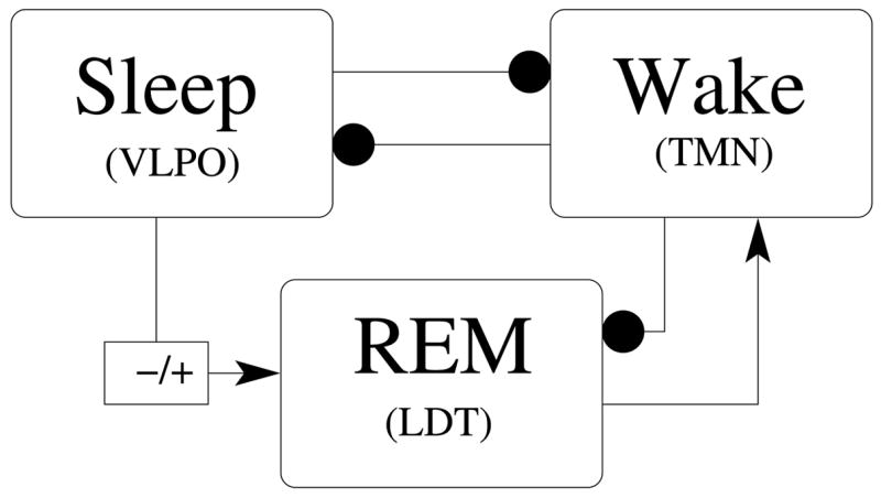
In the 1970s, McCarley and colleagues introduced a dynamic model of sleep cycle alternations between rapid eye movement (REM) and non-REM (NREM) sleep based on a “predator-prey”-like system composed of inhibitory NREM-active populations and excitatory REM-active populations [22]. Since this early model, much experimental work, involving standard physiological techniques [?, 28, 25, 30, 19, 18] and genetic approaches [?, 24], has established the neurophysiology involved in the control of sleep-wake behavior: in particular, mutually inhibitory sleep- and wake-active neuronal populations in the brainstem and hypothalamus are implicated in the production of sleep and wake, respectively. Saper and colleagues have proposed a conceptual model in which mutual inhibition between sleep- and wake-active neuronal populations represents a flip-flop switch that governs the dynamics of sleep-wake transitions [28]; however, formal modeling of behavioral state control has not yet integrated this new information.

In experimental studies, sleep-wake behavior is often summarized as total percentages of wake, NREM sleep, and REM sleep and mean durations of bouts. Although this information is useful for identifying hyper-/hyposomnias or differences between light and dark periods, it does not address the finer architecture of sleep-wake behavior. A detailed characterization of this architecture is necessary when considering the control of wake and sleep at the neuronal level: thus, we consider distributions of bout durations and organization of sleep-wake behavior in addition to traditional measures. By describing mouse sleep-wake behavior in these terms, we specify measures for model performance.

In contrast to the single consolidated night-time sleep bout typically experienced by adult humans, adult mice exhibit polyphasic sleep-wake behavior (Figure 1). In addition to the sustained bouts of wakefulness associated with feeding and locomotor behavior, many species, including mice, normally experience brief awakenings from sleep. In the past, such brief awakenings were often discounted as “noise”; however, they are increasingly recognized as an important part of sleep architecture [7].

Figure 1.

Hypnograms summarize 2 hours of typical experimentally observed alternations between wake (W), sleep (S), and REM sleep (R). If brief awakenings are neglected (left), the polyphasic sleep-wake structure is evident. Including brief awakenings (right), illustrates the qualitative differences between brief and sustained awakenings.

Statistical analyses of distributions of sleep and wake bout durations in multiple species have established that sleep bout durations obey an exponential distribution, and (rodent) wake bout durations obey a “power law with a tail” distribution [17]. The distinction between the regime of wake bout durations in which the power law holds and the regime considered to be the “tail” forms an emergent, species-dependent threshold (occurring at 2 minutes in mice) separating brief and sustained wake bouts. Furthermore, this distinction suggests a mechanistic dichotomy between brief and sustained wake bouts [17, 12].

In the present work, we propose a deterministic model of the sleep-wake network. Specifically, we examine dynamics arising from interactions among wake-, sleep-, and REM-active populations to elucidate mechanisms whereby this network may control behavioral states. By considering sleep-wake behavior in the context of neuronal population activity, we incorporate tenets derived from previous modeling of sleep-wake behavior on the phenomenological [2, ?] or biophysical [6, 13] levels while targeting the role of network dynamics in behavioral state control. Thus, our model provides a novel framework for exploring dynamical principles that may underlie normal sleep-wake physiology as well as physiology that may be altered in pathologic states like narcolepsy.

3 Materials and Methods

Summary of relevant physiology

We introduce a deterministic model of the mouse sleep-wake network. Our definition of the sleep-wake network includes locus coeruleus (LC), tuberomammillary nucleus (TMN), dorsal raphe (DR), extended ventrolateral preoptic nucleus (eVLPO), ventrolateral preoptic cluster (VLPO), laterodorsal tegmental nucleus (LDT), and pedunculopontine tegmental nucleus (PPT). Each of these neuronal populations demonstrates state-dependent firing profiles with rapid transitions between high and low firing rates. Causal relationships between the activity of a given population and a particular behavioral state have been established through extensive experimentation with site-specific lesions and neurotransmitter agonists and antagonists.

We classify each neuronal population as wake-active, sleep-active, or REM-active based on the state in which the population is maximally active; our sleep-active designation refers to maximal activity during both NREM and REM sleep. Neuronal (sub-) populations that are equally active in more than one of these categories (wake, sleep, REM sleep) are not included in our network; we assume that the effects of populations with non-specific behavior are collectively described by multiple populations with state-specific behavior. For example, LDT includes a subpopulation of neurons that is active during both wake and REM sleep and a subpopulation of neurons that is active during REM sleep only [5]: by assuming that the effects of LDT activity during wakefulness are described by the activity of other (exclusively) wake-active populations, we can consider LDT to denote its REM-active subpopulation.

Table 1 summarizes neuronal populations of the sleep-wake network and their associated neurotransmitters; populations are grouped by the state in which they are maximally active.

Table 1.

Relevant neuronal populations by state of maximal activity

Active state	Neuronal population	Neurotransmitters
Wake	Tuberomammillary nucleus (TMN)	Histamine
	Locus coeruleus (LC)	Norepinephrine
	Dorsal raphe (DR)	Serotonin
Sleep	Ventrolateral preoptic cluster (VLPO)	GABA/Galanin
	Extended ventrolateral preoptic nucleus (eVLPO)	GABA/Galanin
REM only	Laterodorsal tegmental nucleus (LDT)	Acetylcholine
	Pedunculopontine tegmental nucleus (PPT)	Acetylcholine
Wake only	Lateral hypothalamic neurons (LHA)	Orexin

Modeled wake-active populations include LC, DR, and TMN. LC and DR are monoaminergic neuronal nuclei located in the brainstem that have long been associated with maintaining muscle tone and promoting vigilance [1, 10]. The primary neurotransmitters of LC and DR neurons are norepinephrine (NE) [1] and serotonin (5-HT) [33], respectively. The TMN is a hypothalamic nucleus that represents the sole source of histamine in the brain [28].

Although orexin neurons are most active during wakefulness, properties such as firing profile [15, 23], elevated resting membrane potential [8], and self-excitation [16] differentiate orexin neurons from other wake-active populations. Therefore, we do not consider orexin neurons to be one of the modeled wake-active populations (the functional role of these cells is analyzed in a separate manuscript).

Modeled sleep-active populations include the GABAergic/galaninergic VLPO and eVLPO. There is significant evidence suggesting that the VLPO and eVLPO form an important sleep center in the brain [30, 19]. Although the distinction between VLPO cluster and eVLPO is not unanimously recognized, Saper, Lu, and colleagues have identified anatomic and functional differences between the two: anatomic differences are based on cell density and efferent projections, while functional differences suggest that activity (as measured by the expression of fos) in the VLPO core is highly correlated with NREM sleep and activity in the eVLPO is highly correlated with REM sleep [18]. Modeled REM-active populations include subpopulations of the LDT/PPT. As previously noted, neurons in LDT/PPT exhibit a range of firing profiles, but we focus on those that are active during REM sleep only. Cholinergic signalling from neurons in LDT/PPT has been directly linked to REM sleep through a range of experiments [4, 31].

Although we do not include a separate population of GABAergic REM-active neurons in our model, there is a mechanism for increasing the strength of (GABAergic) inhibition to the wake-active populations immediately preceding and during each REM bout. We attribute this increased inhibition to activation of the eVLPO [18], but other GABAergic populations [21, 20] may be responsible.

Model formulation

From the physiology reviewed above, we extracted a reduced network of three coupled wake-, sleep-, and REM-active neuronal populations (denoted $\mathcal{W},\hspace{0.17em}\mathcal{S}$, and $\mathcal{R}$, respectively) as shown in Figure 2. The activity of each population in the reduced network is modeled by Morris-Lecar relaxation equations [26]. Coupling between populations was based on experimentally-determined anatomic connections. The strength of inhibition/excitation between model populations is modulated by scaling variables representing homeostatic sleep drives.

Figure 2.

Nullclines of the form associated with Morris-Lecar-type equations have three distinct configurations determined by the branch of the cubic on which the intersection point is located: left branch (top, left), right branch (top, right), or middle branch (bottom).

Conductance-based Morris-Lecar equations are a lower-dimensional form of Hodgkin-Huxley-type single-cell models [14]. A single gating variable on the potassium current yields a 2-dimensional system of equations. For $j=\mathcal{W},\hspace{0.17em}\mathcal{S},\hspace{0.17em}\mathcal{R}$, the model equations have the form

$$\begin{array}{l}\frac{d{v}_j}{dt}=f(v_j,u_j)\\ \frac{d{u}_j}{dt}=\epsilon g(v_j,u_j)\end{array}$$

where 0 < ε ≪ 1; population-dependent parameters determine different intrinsic properties for $\mathcal{W},\hspace{0.17em}\mathcal{S}$, and $\mathcal{R}$. The “smallness” of ε quantifies the order of magnitude separating rates of change in v_j and u_j and introduces two time scales: t and εt. The fast rate of change in v_j permits the model to describe activity on multiple time scales: as previously described, population activity levels change quickly between states and slowly within states. Since Morris-Lecar equations are usually associated with single-cell activity rather than population activity, the time scales associated with our modified Morris-Lecar oscillators are much slower than time scales in the original Morris-Lecar equations. The full model equations are presented in the Appendix.

In our context, v_j describes the activity of population j, and u_j is a recovery variable associated with oscillatory and excitable properties intrinsic to each population [12, 9, 35]. Because we assume that each population is tonically active in the absence of coupling, these properties are not significant in the uncoupled context; however, they are very important to the network dynamics arising from the full system of coupled equations.

From the class of relaxation oscillator equations, the Morris-Lecar equations were selected for their geometric properties. In particular, the shape of the nullclines associated with the Morris-Lecar equations is important to our analysis. Typically, nullclines separate regions of the vu–phase plane in which u and v are increasing or decreasing and give insight into the qualitative behavior of solutions of the system of equations. Taking all other variables to be fixed, nullclines N_v and N_u describe the values of v and u for which the equations dv/dt and du/dt are zero:

$$\begin{array}{l}{N}_v=\{(v,u)|v^{\prime }=0\}\\ N_u=\{(v,u)|u^{\prime }=0\}\end{array}$$

In the associated vu–phase plane, N_v has a standard cubic shape while N_u is sigmoidal. Nullclines of this form may assume three possible distinct relative configurations (Figure 2). The location of the point p at which N_v and N_u intersect specifies default behavior of the associated population and varies with behavioral state:

• p on left branch of N_v: both v and u values are close to (v, u)-coordinates of p; in this case, these values are low and thus, this nullcline configuration corresponds to low population activity.

• p on middle branch: v and u oscillate; therefore, this nullcline configuration corresponds to oscillatory activity.

• p on right branch: both v and u values are close to (v, u)-coordinates of p; in this case, these values are high and thus, this nullcline configuration corresponds to high population activity.

We assume that all populations are active in the absence of coupling (p on right branch); coupling effects give rise to the other nullcline configurations, and this geometry underlies the fundamental dynamics of the network.

Connectivity of the model network

Connectivity of the model network, summarized in Figure 2, is based on anatomical connectivity of the neuronal populations of the sleep-wake network and gives rise to population-specific coupling effects, denoted by c_j, in the dv_j/dt equations:

$$\frac{d{v}_j}{dt}=f(v_j,u_j)+c_j$$

with

$$\begin{array}{l}{c}_S=-g_W(t_W)(1-h)+n_S\\ c_W=\{\begin{array}{ll}-g_S(t_S)-g_{a_{LC}}(v_W-\mathit{aLC})-g_{eV}{e}_V+n_W\hfill & \text{during\hspace{0.17em}NREM\hspace{0.17em}sleep}\hfill \\ -g_S(t_S)\hfill & \text{otherwise}\hfill \end{array}\\ c_R=\{\begin{array}{ll}-g_S(t_S)+g_{LC}r\hspace{0.17em}{e}_V+n_R\hfill & \text{during\hspace{0.17em}sleep}\hfill \\ -g_W(t_W)+n_R\hfill & \text{during\hspace{0.17em}wake}\hfill \end{array}\end{array}$$

where h, r, and e_V are scaling variables; g_W,S(t_W,S) are continuous activation functions of time elapsed since the onset of the wake or sleep bout, respectively; n_W,S,R are noise terms; and g_aLC and a_LC are constant parameters.

The coupling terms determine the state-dependent nullcline configurations of each population. During NREM sleep, the initial inhibition from $\mathcal{S}$ to $\mathcal{W}$ causes the nullclines associated with $\mathcal{W}$ to assume an oscillatory (rather than inactive) configuration. This choice is based on the intermediate level of activity observed in wake-active populations during NREM sleep and the spontaneous (intrinsic) activity exhibited by these populations [35, ?]. All other coupling terms impose an inactive configuration on the nullclines associated with the postsynaptic population. Our choice of parameters is based on achieving this state-dependent geometry.

State-dependence in these terms occurs because functional coupling effects are predicated on activity of the presynaptic population. Activation may be discrete or continuous: Discrete activation is modeled by a Heaviside function, H(v_p), of activity in the presynaptic population, v_p, and specifies the state-dependent cases. (H(v_p) = 1 for v_p ≥ 0, H(v_p) = 0 otherwise.) Continuous activation is modeled as a smooth saturating function of the time, t_W,S, elapsed since the activation of the presynaptic population, tanh(ρ_W,St_W,S) with parameters ρ_W,S. Since we use a single set of relaxation oscillation equations to describe the activity of an entire population, ρ_W,S governs the rate of population recruitment inherent in activation of the population.

The behavioral state of the network is classified by the heuristic activity level of $\mathcal{W},\hspace{0.17em}\mathcal{S}$, and $\mathcal{R}$. If v_W or v_R exceed the “activity threshold” delimiting the onset of population activity, then the network is assumed to be in wake or REM sleep, respectively. The network enters NREM sleep when v_S exceeds the activity threshold and v_W and v_R do not. By imposing additional conditions for NREM sleep, we eliminate ambiguity in scoring of simulated behavioral states. For the results presented herein, zero is taken to be the “activity threshold”; however, because onset and offset of activity in these populations is fast, there is minimal dependence on the choice of threshold separating active and inactive states.

Homeostatic sleep drives and scaling variables

The initiation and consolidation of human sleep have been modeled as the interaction of circadian and homeostatic drives known as process C and process S, respectively [2]. Circadian drive influences behavior according to time of day while homeostatic sleep drives help maintain fixed daily amounts of NREM and REM sleep by promoting sleep in proportion to preceding waking behavior. The two-process model has been adapted to other mammals [37], including those with polyphasic sleep-wake behavior, by identifying species-specific time courses for homeostatic sleep drive and modifying effects of circadian drive.

Because sleep-wake behavior persists in the absence of a functional circadian pacemaker, we make the simplifying assumption that circadian drives constitute a modulation, rather than an intrinsic dynamic element, of behavioral state control. Therefore, in the present study, we restrict our focus to network dynamics driven by homeostatic effects.

Selective sleep deprivation protocols suggest the existence of separate NREM and REM homeostatic sleep drives. Agents of REM homeostasis remain unknown, but several factors have been proposed to mediate NREM drive [34, 27]. The best studied of these is adenosine. Adenosine concentrations rise during waking and fall during sleep. High adenosine levels reduce the frequency of inhibitory post-synaptic potentials (IPSPs) on VLPO neurons [25, 3], thus providing a mechanism for the production of sleep. Adenosine may also act through other mechanisms [34, 29], and much remains to be learned about sleep-promoting factors in general.

Based on our understanding of adenosine, we model homeostatic sleep drive by introducing a variable h that rises during wakefulness, falls during sleep, and scales the strength of inhibition from $\mathcal{W}$ to $\mathcal{S}$. The behavior of h is effectively described by

$$\frac{dh}{dt}=\{\begin{array}{ll}\frac{2-h}{{\tau }_{hW}}\hfill & \text{during\hspace{0.17em}wakefulness}\hfill \\ -\frac{h}{{\tau }_{hS}}\hfill & \text{during\hspace{0.17em}sleep}\hfill \end{array}$$

where τ_hW and τ_hS are time constants controlling the growth and decay of h during wake and sleep, respectively, and H(x) denotes the Heaviside function. Additional subtleties of the dh/dt equation are described in the Appendix. To obtain the appropriate reduction in inhibition from $\mathcal{W}$ to $\mathcal{S}$, g_W (t_W ) is multiplied by (1−h) in c_W; hence, the strength of inhibition from $\mathcal{W}$ to $\mathcal{S}$ varies inversely with h.

In the absence of an identified agent of REM homeostasis, our implementation of REM homeostatic drive is based on phenomenological observations pertaining to REM sleep. Experiments suggest that the occurrence of REM sleep is associated with both excitation (or disinhibition) of REM-active populations and a gating mechanism involving a reduction of activity in wake-active populations. Therefore, we model REM homeostatic sleep drive as a REM-promoting force composed of two processes, r_f and r_s, acting on different time scales; our implementation is based on a model proposed by Franken [11]. Total REM homeostatic sleep drive is described by r = r_f +r_s. The fast process, denoted r_f in our model, is involved in timing REM sleep within a sleep bout and is governed by

$$\frac{d{r}_f}{dt}=\{\begin{array}{ll}\frac{r_{\infty }-r_f}{{\tau }_{rf}}\hfill & \text{during\hspace{0.17em}sleep}\hfill \\ 0\hfill & \text{otherwise}\hfill \end{array}$$

where r_∞ and τ_rf are parameters describing the maximal value and time constant of r_f, respectively; r_f is reset to zero by the occurrence of a REM bout.

The slow process, denoted r_s in our model, regulates the daily amount of REM sleep and is governed by

$$\frac{d{r}_s}{dt}=\{\begin{array}{ll}-\frac{1}{\beta }\hfill & \text{during\hspace{0.17em}REM\hspace{0.17em}sleep}\hfill \\ \frac{1}{\alpha }\hfill & \text{otherwise}\hfill \end{array}$$

where parameters α and β control the rate of growth and decay of r_s.

The gating mechanism involving reduced activity in wake-active populations is modeled with the variable e_V ; e_V scales both inhibition to $\mathcal{W}$ and excitation to $\mathcal{R}$. The latter represents disinhibition of $\mathcal{R}$ occurring as a result of decreased activity in the monoaminergic populations represented by $\mathcal{W}$. The variable e_V is governed by

When $\mathcal{W}$ is active, e_V does not change; however, when activity in $\mathcal{W}$ drops, e_V grows according to

$$\frac{d{e}_V}{dt}=\{\begin{array}{ll}\frac{1-e_V}{{\tau }_{eV}}\hfill & \text{when\hspace{0.17em}W\hspace{0.17em}is\hspace{0.17em}inactive}\hfill \\ 0\hfill & \text{otherwise}\hfill \end{array}$$

where τ_eV is a parameter controlling the rate of growth of e_V ; the occurrence of a REM bout resets e_V to 0.

Numerical implementation

To reproduce the “noisiness” inherent in any biological system, we introduced stochastic terms into four of the differential equations in our system: $\frac{dh}{dt}$ and $\frac{d{v}_j}{dt}$ for $j=\mathcal{W},\hspace{0.17em}\mathcal{S}$, and $\mathcal{R}$. The stochastic terms were normally distributed with mean 0 and variance 0.25, 1, 1, and 20, respectively; at each time step, new values were generated for the stochastic terms, and the differential equations were modified accordingly.

All simulations were run on a Linux workstation using the ordinary differential equation (ODE) solver XPPAUT, developed by G. B. Ermentrout and available at ftp://ftp.math.pitt.edu/pub/bardware. A Runge-Kutta integration method with step size 0.01 was used for all simulations. Simulation output was analyzed using code written in MATLAB (The Mathworks Inc., Natick, MA, USA).

4 Results

In the absence of noise, the dynamics of our model network give rise to a stereotypical sequence of behavior. The geometry of the system permits analysis of this solution that identifies the dynamic mechanisms underlying state transitions and suggests separate mechanisms for brief and sustained wake bouts. With the addition of noise, our parameter regime generates simulated behavior consistent with experimentally observed mouse sleep-wake data. We address these two aspects of our results in two separate sections.

Simulated mouse sleep-wake behavior

Typical simulated mouse behavior is summarized in Figure 5. In addition to qualitative comparisons, with our trivial implementation of noise our model can reproduce experimentally observed relative proportions of wake, NREM sleep, and REM sleep; number and duration of bouts; and realistic sleep architecture as measured by transition probabilities.

Figure 5.

Hypnograms of typical simulated mouse sleep-wake behavior capture both the polyphasic nature of sustained wake bouts (left) and the qualitative differences between brief and sustained wake bouts (right).

We compare the simulated behavior described by our model with experimental data provided courtesy of Mochizuki and colleagues (n=8). The experimental data was previously published in [24], and a discussion of methods used to collect this data are described therein. All simulated behavior was generated using a single set of parameters. Model robustness to variation of parameters is addressed in the following section.

Daily percentages of wake, NREM sleep, and REM sleep

Our model can reproduce experimentally observed daily (24 hour) percentages of time spent in wake, NREM sleep, and REM sleep as seen in Figure 6. By considering percentages of time spent in each behavioral state over 24 hours, we mitigate circadian phase dependence to reveal underlying homeostatic equilibria. The model produces slightly less REM sleep than is experimentally observed; the source of this difference is a discrepancy in the duration, rather than the raw number, of REM bouts between the model and the experimental data. The close agreement between our model results and experimental data for daily percentages of wake, NREM sleep, and REM sleep suggests that the homeostatic drives in the model are tuned to biophysically reasonable equilibrium values.

Figure 6.

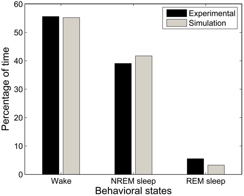
There is close agreement between experimental and simulated data in the percentage of time spent in each behavioral state.

Number and duration of bouts

Because mouse sleep-wake behavior is polyphasic, daily amounts of wake, NREM sleep, and REM sleep are composed of many bouts of varying lengths. Scoring behavior in 10 second epochs, Mochizuki and colleagues identified mean numbers and durations for bouts of each behavioral type. As described in the Introduction, we will consider brief and sustained wake bouts separately.

The average numbers of bouts of each behavioral type are shown in Figure 7. There is good agreement between the model and the experimental data, though the model has fewer brief wake bouts than the experimental data.

Figure 7.

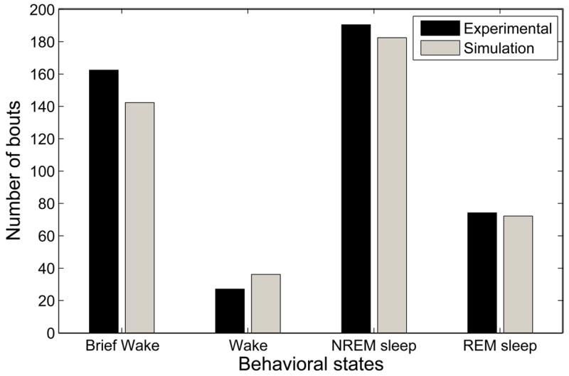
Experimental and simulated data show similar numbers of bouts of each behavioral state.

Mean durations of bouts of each behavioral state are compared in Figure 8. The discrepancy between mean durations of sustained wake bouts occurs because our model lacks circadian effects that promote very long wake bouts. Mean bout durations for the other behavioral states show close agreement. The large variance of the bout duration data renders mean bout duration an insufficient characterization of bouts; therefore, we compare histograms of simulated and experimentally observed behavior.

Figure 8.

Mean bout durations for each behavioral state are similar between experimental and simulated data.

Histograms comparing wake bout durations in model output and experimental data (Figure 9) show that the model captures the relative frequency of each type of wake bout. We measure durations in minutes instead of seconds because very extended wake bout durations occur during the dark period. The slightly lower number of brief (0–2 min) wake bouts in model data may be due to the absence of brief awakenings occurring in response to uncontrolled environmental factors (occasional noise, vibration, etc.).

Figure 9.

Distribution of wake bout durations in experimental and simulated data show close agreement.

Histograms comparing NREM sleep bout durations in model output and in experimental data are shown in Figure 10. There is good qualitative agreement between the model and experimental data: bouts of NREM sleep are most likely to be less than 120 seconds in duration, and nearly all bouts of NREM sleep fall in the range from 0–480 seconds in duration. There is a lower incidence of NREM bouts of duration 120–240 seconds and a higher incidence of NREM bouts of duration 240–480 seconds in the model compared to the experimental data; additional noise in the model, particularly random external stimuli, may fracture some of these longer bouts into bouts of shorter duration.

Figure 10.

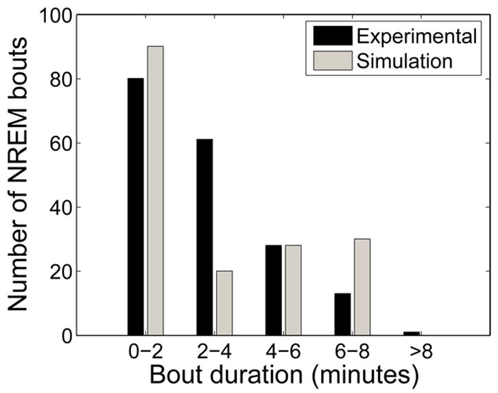
Simulated data captures features of experimental distribution of NREM sleep bout durations.

Histograms comparing REM bout durations in model output and experimental data are shown in Figure 11. Most REM bouts fall in the first two bins (0–40 seconds and 40–80 seconds) in both the model output and the experimental data. However, longer REM bouts observed in experimental data are absent in model output. This difference accounts for the discrepancy between the percentage of REM sleep in the model and in the experimental data. The low variance in simulated REM bout durations will be explained in the analysis of the model geometry.

Figure 11.

Comparison of REM sleep bout durations between experimental and simulated data reveals an absence of long REM bouts in simulated data.

Organization of sleep-wake behavior

To quantify the organization of sleep-wake behavior, we compute probabilities of transitioning from one behavioral state to another (given that a state transition occurred). Stereotyped sleep-wake patterns that emerge are often conserved across species: some transitions (e.g., wake → REM sleep) are never seen in normal behavior and can be considered “inappropriate”, while others (e.g., NREM sleep → REM sleep) are common. Transition probabilities for simulated and experimental data (Figure 12) show similar structure; no inappropriate state transitions are produced by the model.

Figure 12.

State transition probabilities in simulated behavior are similar to the probabilities calculated from experimental data.

In addition to specific transitions from one state to another, stereotypical sequences of behavior are observed experimentally and clinically. One such sequence is the progression from NREM sleep to REM sleep to brief wakefulness and back to NREM sleep [7]. This sequence is observed repeatedly in our simulated behavior.

Model geometry and predictions

To better understand dynamic principles of the network and mechanisms of transition between states, we analyzed the mathematical structure of the network equations in the absence of noise. Complete mathematical details are beyond the scope of this paper, but the Methods section provides an overview of our approach. By exploiting both the separation of time scales within the network equations and the state-dependent “importance” of variables, we were able to reduce the dimension of the system in a state- and population-dependent manner. This strategy allowed us to examine network dynamics in terms of nullclines associated with population variables, and it provided a structured framework for understanding parameter dependence in our model.

Mechanisms for state transitions

The stereotypical sequence of behavior consists of a sustained wake bout and an extended sleep bout composed of two NREM-REM sleep cycles and four brief awakenings. We describe the predicted mechanisms for each of these state transitions.

The transition from wake to (NREM) sleep is initiated by the NREM homeostatic sleep drive, described by the variable h. Recall that h increases during wakefulness, and the strength of inhibition from $\mathcal{W}$ to $\mathcal{S}$ varies inversely with h. When the strength of inhibition is no longer sufficient to prevent the onset of activity in $\mathcal{S}$, the “flip-flop” switch flips: $\mathcal{S}$ activates and inhibition from $\mathcal{S}$ to $\mathcal{W}$ is initiated (Figure 12). In the coupled oscillator literature, this mechanism is known as “intrinsic escape” [?, 32].

Recall that the onset of inhibition from $\mathcal{S}$ to $\mathcal{W}$ resulted in an oscillatory configuration of $\mathcal{W}$ nullclines. Thus, in contrast to the inactivity observed in $\mathcal{S}$ when it is inhibited by $\mathcal{W}$, activity in $\mathcal{W}$ alternates between high and low levels in an intrinsic relaxation oscillation. We consider the short intervals of high activity in $\mathcal{W}$ to describe brief awakenings; thus, the model suggests that the occurrence of brief awakenings is linked to intrinsic excitability of the wake-active populations. As the sleep bout progresses, short-term REM homeostatic pressure increases the strength of inhibition to $\mathcal{W}$ and the excitation to $\mathcal{R}$. When inhibition to $\mathcal{W}$ is sufficiently strong, the $\mathcal{W}$ nullclines move to an inactive configuration and oscillation in $\mathcal{W}$ ceases. The complete cessation of activity in $\mathcal{W}$ results in further disinhibition of $\mathcal{R}$; if REM homeostatic sleep drive is sufficiently strong, a REM bout occurs.

In our model, a REM bout corresponds to a single excursion (of relaxation oscillation-type) in $\mathcal{R}$; thus, the form and duration of the REM bout result from intrinsic properties of REM-active populations. A combination of excitation and disinhibition permit the intrinsic escape of $\mathcal{R}$; however, the activation of $\mathcal{R}$ completely discharges short-term REM pressure and reduces long-term REM pressure: the resulting drop in total REM pressure reverses both the excitation to $\mathcal{R}$ and the disinhibition of $\mathcal{W}$. Thus, $\mathcal{R}$ returns to relative inactivity after its excursion, and the REM bout activates $\mathcal{W}$ sufficiently to generate a post-REM brief awakening.

The transition from NREM sleep to wake involves a more subtle mechanism than those associated with other state transitions. As previously described, brief episodes of activity in $\mathcal{W}$ result in pulses of inhibition from $\mathcal{W}$ to $\mathcal{S}$. In contrast to the expected behavior of a pure flip-flop switch, this activity does not necessarily transition the network from sleep to sustained wake: instead, switching between states depends on the strength of this pulse. If the pulse sufficiently depresses activity in $\mathcal{S}$, the network will transition from sleep to wake; otherwise, the activity in $\mathcal{W}$ self-terminates with the falling phase of the oscillation, and the sleep bout continues. These possibilities are illustrated in Figure 13.

Figure 13.

Transition from wake to NREM sleep can be understood as intrinsic escape of $\mathcal{S}$: as inhibition from $\mathcal{W}$ to $\mathcal{S}$ decreases as a result of increasing NREM homeostatic sleep drive h, the intersection point of the nullclines, p_S, moves down the left branch of $N_v^S$. It is tracked by the trajectory. When the intersection point loses stability at the knee K_L, the trajectory jumps to the right branch.

The strength of the pulse of inhibition from $\mathcal{W}$ to $\mathcal{S}$ during a brief awakening is determined by the variable h describing NREM homeostatic sleep drive. As h recovers over the course of the sleep bout, the strength of these pulses increases; thus, the value of h during the brief awakening determines whether the network will switch to sustained wake or remain in sleep. Hence, the transition from NREM sleep to sustained wake requires both sufficient recovery in h and the initiation of a brief awakening. This suggests a significant role for intrinsic excitability in the reversibility of sleep.

Model sensitivity to parameters

Our model contains 65 parameters which, based on the variables they modify, fall into three categories: parameters associated with intrinsic properties of $\mathcal{W},\hspace{0.17em}\mathcal{S}$, or $\mathcal{R}$; parameters involved in coupling effects; and parameters associated with homeostatic sleep drives. Because we are able to understand mathematically the nature of state transitions within the model, we gain great insight into the role of each parameter in network dynamics. Thus, rather than attempting to search a 65-dimensional parameter space, we can evaluate the model’s robustness to parameter variation using our analysis of the model dynamics.

In particular, as long as the geometry of the equations is preserved, parameter variation has relatively minor effects on network behavior. Outside these regimes the network dynamics may change drastically. Changes to the first category of parameters affect the shape of the nullclines associated with each population, thus model behavior is very robust to minor changes in these parameters. The second and third categories of parameters are closely involved with mechanisms of state transitions; however, changes to these parameters must alter state-dependent nullcline configurations to significantly alter network dynamics.

Reciprocal inhibition between $\mathcal{W}$ and $\mathcal{S}$, and its relationship to brief awakenings, is a key element of the network structure. Increasing or decreasing the maximal strength of inhibition from $\mathcal{S}$ to $\mathcal{W}$(g_Smax and g_Wmax, respectively) changes the time spent in wake and sleep and the number of brief awakenings observed in stereotypical sequences of behavior. If g_Smax is sufficiently strong to eliminate all brief awakenings, then the network exhibits constant sleep because the transition mechanism from sleep to sustained wake requires brief awakenings.

Similarly, changing the rate of activation from $\mathcal{W}$ to $\mathcal{S}$ affects brief awakenings. If activation is instantaneous or the rate is increased by more than 40%, brief awakenings (with concurrent activity in $\mathcal{W}$ and $\mathcal{S}$) are eliminated and the network rapidly oscillates between wake and NREM sleep. If the rate is decreased, additional brief awakenings occur. Network behavior is not sensitive to changes in the rate of activation from $\mathcal{S}$ to $\mathcal{W}$.

Most of the parameters associated with homeostatic sleep drives (suggestively denoted τ_i) are time constants describing the evolution of variables that scale coupling strengths in the network. Based on the mechanisms of transitions previously discussed, we expect all transitions, with the exception of the transition from the extended sleep bout to the sustained wake bout, to depend smoothly on these parameters. This conclusion is supported by the results of simulation. The exception in smooth dependence arises because, in the absence of noise, the transition from sleep to sustained wake depends on activation of $\mathcal{W}$ in the form of a brief awakening. Although this brief awakening may be intrinsic or post-REM, the transitional brief awakening tends to be one that occurs post-REM bout similar to the brief awakenings that occur at the end of human sleep cycles. Therefore, the duration of extended sleep bouts can change in (discrete) units of sleep cycles rather than continuously.

5 Discussion

We have shown that a network of three coupled relaxation oscillators with variable connectivity can be used to simulate qualitative and quantitative features of mouse sleep-wake behavior including brief and sustained wake, NREM sleep, and REM sleep. Our use of a deterministic model was motivated by our interest in fundamental network dynamics generated by the circuitry of behavioral state control, and our model equations permit formal analysis of the possible mechanisms associated with each state transition.

By implementing the mutual inhibition of the flip-flop switch in the context of coupled relaxation oscillators and introducing time courses associated with inhibition onset, our approach captures the salient features of the conceptual model of a sleep-wake switch (two stable states with minimal time spent in intermediate states [28]) and incorporates features associated with the robustness necessary in a physiological system. A pure flip-flop switch mechanism is subject to inappropriate transitions in the presence of noise: in behavioral state control, such inappropriate transitions would translate to potentially dangerous switches between wake and sleep.

Architecture of sleep-wake behavior

A major feature of our model is its ability to describe the finer architecture of mouse sleep-wake behavior. In the phenomenological tradition of sleep modeling, brief awakenings were necessarily ignored: the duration of brief awakenings cannot logically be linked to sleep homeostasis. Recently, Tamakawa and colleagues described a model of rat sleep-wake behavior based on the concept of the sleep-wake switch and involving similar physiology [36]. Their model produces alternations between bouts of wake and sleep that have been matched to mean durations of wake and sleep bouts. Although they successfully translated the concepts of behavioral state control into a biophysical context, they did not attempt to reproduce the finer architecture of sleep-wake behavior.

By contrast, our model can reproduce distributions of bout durations and probabilities of transitions between states. In particular, by specifying an oscillatory regime of the wake-active neuronal population, we obtain wake bouts with durations that are governed by intrinsic properties of the population rather than homeostatic sleep drive. In the absence of this oscillatory regime, brief awakenings could be obtained by short, random excitation of the wake-active populations; this type of stimuli is associated with uncontrolled environmental factors. As previously mentioned, this type of brief awakening may be responsible for the slightly lower number of brief awakenings in the simulated behavior compared to the experimental data. However, the high incidence of brief awakenings throughout sleep suggests that environmental factors are not exclusively responsible. The intrinsic occurrence of brief awakenings in our model is consistent with the idea that regular periods of awareness during sleep act as a safety measure to offset the vulnerability of decreased sensory perception during sleep [12].

Concurrent activity in wake- and sleep-active populations

Because our simulated brief awakenings represent concurrent activity in wake- and sleep-active populations, our model suggests that VLPO neurons may be active during brief awakenings. This idea depends crucially on properties of our “biological flip-flop” since concurrent activity is impossible in a pure flip-flop switch. Experimental evidence using fos to measure neuronal activity has shown that VLPO neurons are active during sleep and minimally active during sustained awakenings; however, the time resolution of fos techniques is not sufficient to determine the activity level of VLPO neurons during brief awakenings. Without recordings from VLPO neurons in behaving rodent models, we cannot assume that (brief) wakefulness and activity of VLPO neurons are mutually exclusive.

NREM-REM flip-flop?

Lu and colleagues have recently proposed a conceptual model for NREM-REM alternation involving mutual inhibition between GABAergic REM-on (sublaterodorsal nucleus) and REM-off (ventrolateral part of periaqueductal grey matter and lateral pontine tegmentum) populations [20]. In this conceptual framework, increased activity in eVLPO inhibits monoaminergic populations, thereby removing excitation from REM-off populations and resulting in disinhibition of REM-on populations. Although our implementation of NREM-REM alternation within the sleep cycle is based on the classical view of interactions between REM-off monoaminergic populations and REM-on cholinergic populations [22, ?], our model is consistent with the theory that increased activity in the eVLPO results in disinhibition of REM-on neurons. In our current implementation, this disinhibition is not mediated through REM-off neurons; however, because the REM-off population may be involved in other regulatory aspects of REM phenomena [20], we may need to extend our model to include a REM-off intermediary population in future work.

Technical considerations and future directions

A limitation of the relaxation oscillator formalism is the robustness of relaxation oscillations in the presence of noise. Although our trivial implementation of noise was sufficient to reproduce many statistical features of mouse sleep-wake behavior, the durations of simulated brief awakenings and REM bouts tended to be normally distributed around the fixed durations associated with the $\mathcal{W}$ and $\mathcal{R}$ equations, respectively. By conducting a formal analysis of the implementation of noise, including an assessment of the type of noise used and the placement of stochastic terms in the model equations, we may be able to improve some of these statistical features of the simulated data.

In addition, we plan to use this model framework to explore modified sleep-wake behavior that occurs in pathologic states such as narcolepsy, as well as normal variation in sleep-wake behavior over the course of the day. Certain experimentally observed features, such as extended wake bouts at the onset of the dark period and non-uniform distribution of REM sleep, do not occur in our model. These features, along with hourly variation in amounts of wake and sleep, are probably dependent on circadian effects. The interaction between the circadian system and sleep-wake behavior has been studied extensively, and recent experiments have established some of the anatomy involved in this interaction. In future work, we plan to implement circadian effects into our model; in addition to improving the agreement between simulated and experimental data, this implementation will provide an excellent opportunity to explore the physiologic role of the circadian system in modulating sleep-wake dynamics.

Figure 3.

Summary of model sleep-wake network architecture: filled circles denote inhibitory connections; arrows denote excitatory connections. The sign change on the projection from $\mathcal{S}$ to $\mathcal{R}$ represents the net effect of the projection from eVLPO to LDT-PPT: this projection is thought to synapse on inhibitory interneurons in LDT-PPT, thereby disinhibiting the (excitatory) cholinergic neurons in LDT-PPT and exerting a net excitatory effect.

Figure 4.

Activation functions for coupling effects can be discrete (top) or continuous (bottom).

Figure 14.

Because activation of inhibition from $\mathcal{W}$ to $\mathcal{S}$ is associated with a time course, there is a regime in which brief awakenings occur without switching network behavior.

6 Appendix

Model equations

The activity of each population is modeled by the following modified Morris-Lecar equations:

$$\begin{array}{l}{v}_i^{\prime }=-g_L(v_i-E_L)-g_{Ca}{m}_{\infty }(v_i)(v_i-E_{Ca})-g_K{w}_i(v-E_K)+\sum _{j\ne i}{\text{coupling}}_j\\ w_i^{\prime }=\phi (w_{\infty }(v_i)-w_i)/{\tau }_w(v_i)\end{array}$$

where $i,\hspace{0.17em}j=\mathcal{W},\hspace{0.17em}\mathcal{S},\hspace{0.17em}\mathcal{R}$ and g_L, E_L, g_Ca, E_Ca, g_K, E_K, and φ are constant parameters. The equations for m_∞(v), w_∞(v), and τ_w(v) are given by

$$\begin{array}{c}{m}_{\infty }(v_i)=(1+exp(-(v_i-{\alpha }_m)/{\beta }_m)){)}^{-1}\\ w_{\infty }(v_i)={(1+exp(-(v_i-{\alpha }_w)/{\beta }_w))}^{-1}\\ {\tau }_w(v_i)={(cosh((v_i-{\alpha }_w)/(2{\beta }_w)))}^{-1}\end{array}$$

where α_m,w and β_m,w are constants.

$$\begin{array}{l}{c}_S=I_S-g_W(t_W)(1-h)+n_S\\ c_W=I_W-g_S(t_S)-g_{\mathit{aLC}}(v_W-\mathit{aLC})H(v_S)H(-v_R)\\ -g_{eV}{e}_{V}H(-v_R)+n_W\\ c_R=I_R-g_S(t_S)H(v_S)-g_W(t_W)(1-H(v_S))\\ +r{g}_{LC}{e}_{V}H(v_W+40)(1-H(v_W+20))+n_R\end{array}$$

where

• I_j describes extra-network drives to the population;

• n_j is normally distributed noise;

• H(·) denotes the Heaviside function (H(x) = 1 for x ≥ 0, H(x) = 0 otherwise);

• t_W and t_S are variables that track the time elapsed since the beginning of the current wake or sleep bout, respectively;

• g_W,S(·) is an activation function describing the onset of inhibition from $\mathcal{W}$ and $\mathcal{S}$, respectively; it has the form g_j(t_W,S) = g_max tanh(ρ_jt_j) where g_max is the (constant) maximal strength of coupling and tanh(ρ_jt_j) is a saturating function of t_j with parameter ρ_j;

• g_eV, g_LC, and g_aLC are constants denoting the maximal strength of the associated coupling term;

• aLC is a constant in the term describing the effects of self-inhibition in LC;

• and h, r, and e_V are scaling variables (described in detail below).

The Heaviside functions in the coupling terms impose state-dependence on coupling effects: i.e., inhibition/excitation are present only when the presynaptic population is active. The activation functions g_W,S(·) capture the effects of population recruitment: the function grows to its maximal value at rate ρ_j as the time elapsed since the beginning of the current wake or sleep bout, t_W,S, increases. The parameter ρ_j describes the rate of population recruitment.

As described in the text, r = r_s + r_f where r_s and r_f are governed by the following equations:

$$r_j^{\prime }=\{\begin{array}{ll}\frac{r_{\infty }-r_f}{{\tau }_{rf}}\hfill & \text{during\hspace{0.17em}sleep}\hfill \\ 0\hfill & \text{otherwise}\hfill \end{array}$$

where r_∞ and τ_rf are constant parameters;

$$r_s^{\prime }=\{\begin{array}{ll}-\frac{1}{\beta }\hfill & \text{during\hspace{0.17em}REM\hspace{0.17em}sleep}\hfill \\ \frac{1}{\alpha }\hfill & \text{otherwise}\hfill \end{array}$$

and the scaling variable e_V is governed by

$$e_V^{\prime }=\frac{1-e_V}{{\tau }_{eV}}$$

where τ_eV is a parameter controlling the rate of growth of e_V

To ensure a robust alternation between extended wake and sleep bouts, the rate of change of h is increased when bout durations exceed a certain threshold. This is accomplished by the addition of the terms

$$\frac{1-h}{({\tau }_{hW}/2)}H(t_W-\text{endWake})$$

and

$$\frac{h}{({\tau }_{hS}/2)}H(t_S-\text{endSleep})$$

to the h′ equation. We set the parameters endWake = endSleep = 20 because experiments suggest that sustained wake and sleep bouts rarely last beyond 20 minutes (with the possible exception of a single, very long wake bout at dark onset). The Heaviside dependence of these terms ensures that they are non-zero only when a wake or sleep bout has lasted beyond 20 minutes; although this rarely occurs, activation of either of these terms increases the rate of growth or decay of h to quickly terminate the bout. Thus, the full equation for h′ is given by

$$\begin{array}{l}\frac{dh}{dt}=\frac{2-h}{{\tau }_{hW}}H(v_W)-\frac{h}{{\tau }_{hS}}H(v_S)\\ +\frac{1-h}{({\tau }_{hW}/2)}H(t_W-\text{endWake})+\frac{h}{({\tau }_{hS}/2)}H(t_S-\text{endSleep})+n_h\end{array}$$

References

- 1.Aston-Jones G, Ennis M, Pieribone V, Nickell WT, Shipley M. The brain nucleus locus coeruleus: Restricted afferent control of a broad efferent network. Science. 1986 November;234(4777):734–737. doi: 10.1126/science.3775363. [DOI] [PubMed] [Google Scholar]
- 2.Borbely AA, Achermann P. Principles and Practice in Sleep Medicine. 4. chapter 14. Saunders/Elsevier; 2005. pp. 787–856. [Google Scholar]
- 3.Chamberlin N, Arrigoni E, Chou TC, Scammell T, Greene R, Saper C. Effects of adenosine on GABAergic synaptic inputs to identified ventrolateral preoptic neurons. Neuroscience. 2003;119:913–918. doi: 10.1016/s0306-4522(03)00246-x. [DOI] [PubMed] [Google Scholar]
- 4.Datta S, Siwek DF. Excitation of the brain stem pedunculopontine tegmentum cholinergic cells induces wakefulness and REM sleep. Journal of Neurophysiology. 1997;77:2975–2988. doi: 10.1152/jn.1997.77.6.2975. [DOI] [PubMed] [Google Scholar]
- 5.Datta S, Siwek DF. Single cell activity patterns of pedunculopontine tegmentum neurons across the sleep-wake cycle in the freely moving rats. Journal of Neuroscience Research. 2002;70:611–621. doi: 10.1002/jnr.10405. [DOI] [PubMed] [Google Scholar]
- 6.Destexhe A, Sejnowski T. Thalamocortical Assemblies. Oxford University Press; 2001. [Google Scholar]
- 7.Dijk DJ, Kronauer RE. Commentary: Models of sleep regulation: successes and continuing challenges. Journal of Biological Rhythms. 1999;14(6):569–573. doi: 10.1177/074873099129000902. [DOI] [PubMed] [Google Scholar]
- 8.Eggermann E, Bayer L, Serafin M, Saint-Mleux B, Bernheim L, Machard D, Jones B, Muhlethaler M. The wake-promoting hypocretin-orexin neurons are in an intrinsic state of membrane depolarization. Journal of Neuroscience. 2003;23(5):1557–1562. doi: 10.1523/JNEUROSCI.23-05-01557.2003. [DOI] [PMC free article] [PubMed] [Google Scholar]
- 9.Endo T, Roth C, Landolt HP, Werth E, Aeschbach D, Achermann P, Borbely AA. Selective REMS deprivation in humans: effects on sleep and sleep EEG. American Journal of Physiology. 1998;274:R1186–1189. doi: 10.1152/ajpregu.1998.274.4.R1186. [DOI] [PubMed] [Google Scholar]
- 10.Espana RA, Scammell TE. Sleep neurobiology for the clinician. SLEEP. 2004;27:811–820. [PubMed] [Google Scholar]
- 11.Franken P. Long-term vs. short-term processes regulating REM sleep. Journal of Sleep Research. 2002;11:17–28. doi: 10.1046/j.1365-2869.2002.00275.x. [DOI] [PubMed] [Google Scholar]
- 12.Halasz P, Terzano M, Parrino L, Bodizs R. The nature of arousal in sleep. Journal of Sleep Research. 2004;13:1–23. doi: 10.1111/j.1365-2869.2004.00388.x. [DOI] [PubMed] [Google Scholar]
- 13.Hill S, Tononi G. Modeling sleep and wakefulness in the thalamocortical system. Journal of Neurophysiology. 2005;93:1671–1698. doi: 10.1152/jn.00915.2004. [DOI] [PubMed] [Google Scholar]
- 14.Hodgkin AL, Huxley AF. A quantitative description of membrane current and its application to conduction and excitation in nerve. Journal of Physiology. 1952;117:500–544. doi: 10.1113/jphysiol.1952.sp004764. [DOI] [PMC free article] [PubMed] [Google Scholar]
- 15.Lee MG, Hassani O, Jones B. Discharge of identified orexin/hypocretin neurons across the sleep-waking cycle. Journal of Neuroscience. 2005;25(28):6716–6720. doi: 10.1523/JNEUROSCI.1887-05.2005. [DOI] [PMC free article] [PubMed] [Google Scholar]
- 16.Li Y, Gao XB, Sakurai T, van den Pol A. Hypocretin/orexin excites hypocretin neurons via a local glutamate neuron-a potential mechanism for orchestrating the hypothalamic arousal system. Neuron. 2002;36:1169–1181. doi: 10.1016/s0896-6273(02)01132-7. [DOI] [PubMed] [Google Scholar]
- 17.Lo CC, Ivanov P, Chou T, Penzel T, Scammell T, Strecker R, Stanley HE. Common scale-invariant pattern of sleep-wake transitions across mammalian species. Proceedings National Academy Science. 2004;101:17545–17548. doi: 10.1073/pnas.0408242101. [DOI] [PMC free article] [PubMed] [Google Scholar]
- 18.Lu J, Bjorkum A, Xu M, Gaus S, Shiromani P, Saper C. Selective activation of the extended ventrolateral preoptic nucleus during rapid eye movement sleep. Journal of Neuroscience. 2002 June;22(11):4568–4576. doi: 10.1523/JNEUROSCI.22-11-04568.2002. [DOI] [PMC free article] [PubMed] [Google Scholar]
- 19.Lu J, Greco MA, Shiromani P, Saper C. Effect of lesions of the ventrolateral preoptic nucleus on NREM and REM sleep. Journal of Neuroscience. 2000 May;20(10):3830–3842. doi: 10.1523/JNEUROSCI.20-10-03830.2000. [DOI] [PMC free article] [PubMed] [Google Scholar]
- 20.Lu J, Sherman D, Devor M, Saper C. A putative flip-flop switch for control of REM sleep. Nature. 2006 doi: 10.1038/nature04767. [DOI] [PubMed] [Google Scholar]
- 21.Maloney KJ, Mainville L, Jones BE. Differential c-fos expression in cholinergic, monoaminergic, and GABAergic cell groups of the pontomesencephalic tegmentum after paradoxical sleep deprivation and recovery. Journal of Neuroscience. 1999;19:3057–3072. doi: 10.1523/JNEUROSCI.19-08-03057.1999. [DOI] [PMC free article] [PubMed] [Google Scholar]
- 22.McCarley R, Hobson JA. Neuronal excitability modulation over the sleep cycle: A structural and mathematical model. Science. 1975 July;189(4196):58–60. doi: 10.1126/science.1135627. [DOI] [PubMed] [Google Scholar]
- 23.Mileykovskiy B, Kiyashchenko L, Siegel J. Behavioral correlates of activity in identified hypocretin/orexin neurons. Neuron. 2004;46:787–798. doi: 10.1016/j.neuron.2005.04.035. [DOI] [PMC free article] [PubMed] [Google Scholar]
- 24.Mochizuki T, Crocker A, McCormack S, Yanagisawa M, Sakurai T, Scammell T. Behavioral state instability in orexin knock-out mice. Journal of Neuroscience. 2004 July;24(28):6291–6300. doi: 10.1523/JNEUROSCI.0586-04.2004. [DOI] [PMC free article] [PubMed] [Google Scholar]
- 25.Morairty S, Rainnie D, McCarley R, Greene R. Disinhibition of ventrolateral preoptic area sleep-active neurons by adenosine: a new mechanism for sleep promotion. Neuroscience. 2004;123:451–457. doi: 10.1016/j.neuroscience.2003.08.066. [DOI] [PubMed] [Google Scholar]
- 26.Morris C, Lecar H. Voltage oscillations in the barnacle giant muscle fiber. Journal of Biophysiology. 1981;35:193–213. doi: 10.1016/S0006-3495(81)84782-0. [DOI] [PMC free article] [PubMed] [Google Scholar]
- 27.Porkka-Heiskanen T, Strecker RE, McCarley RW. Brain site-specificity of extracellular adenosine concentration changes during sleep deprivation and spontaneous sleep: an in vivo microdialysis study. Neuroscience. 2000;99:507–517. doi: 10.1016/s0306-4522(00)00220-7. [DOI] [PubMed] [Google Scholar]
- 28.Saper C, Chou T, Scammell T. The sleep switch: hypothalamic control of sleep and wakefulness. Trends in Neurosciences. 2001 December;24(12):726–731. doi: 10.1016/s0166-2236(00)02002-6. [DOI] [PubMed] [Google Scholar]
- 29.Scammell TE, Gerashchenko DY, Mochizuki T, McCarthy MT, Estabrooke IV, Sears CA, Saper CB, Urade Y, Hayaishi O. An adenosine a2a agonist increases sleep and induces fos in ventrolateral preoptic neurons. Neuroscience. 2001;107:653–663. doi: 10.1016/s0306-4522(01)00383-9. [DOI] [PubMed] [Google Scholar]
- 30.Sherin JE, Elmquist J, Torrealba F, Saper C. Innervation of histaminergic tuberomammillary neurons by GABAergic and galaninergic neurons in the ventrolateral preoptic nucleus of the rat. Journal of Neuroscience. 1998 June;18(12):4705–4721. doi: 10.1523/JNEUROSCI.18-12-04705.1998. [DOI] [PMC free article] [PubMed] [Google Scholar]
- 31.Siegel J. Clues to the functions of mammalian sleep. Nature. 2005 October;437(27):1264–1271. doi: 10.1038/nature04285. [DOI] [PMC free article] [PubMed] [Google Scholar]
- 32.Skinner F, Kopell N, Marder E. Mechanisms for oscillation and frequency control in reciprocally inhibitory model neural networks. Journal of Computational Neuroscience. 1994;1:69–87. doi: 10.1007/BF00962719. [DOI] [PubMed] [Google Scholar]
- 33.Steininger TL, Wainer BH, Blakely RD, Rye DB. Serotonergic dorsal raphe nucleus projections to the cholinergic and noncholinergic neurons of the pedunculopontine tegmental regions: a light and electron microscopic anterograde tracing and immunohistochemical study. Journal of Comparative Neurology. 1997;382:302–322. doi: 10.1002/(sici)1096-9861(19970609)382:3<302::aid-cne2>3.0.co;2-7. [DOI] [PubMed] [Google Scholar]
- 34.Strecker RE, Morairty S, Thakkar MM, Porkka-Heiskanen T, Basheer R, Dauphin LJ, Rainnie DG, Portas CM, Greene RW, McCarley RW. Adenosinergic modulation of basal forebrain and preoptic/anterior hypothalamic neuronal activity in the control of behavioral state. Behavioral Brain Research. 2000;115:183–204. doi: 10.1016/s0166-4328(00)00258-8. [DOI] [PubMed] [Google Scholar]
- 35.Taddese A, Bean BP. Subthreshold sodium current from rapidly inactivating sodium channels drives spontaneous firing of tuberomammillary neurons. Neuron. 2002;33:587–600. doi: 10.1016/s0896-6273(02)00574-3. [DOI] [PubMed] [Google Scholar]
- 36.Tamakawa Y, Karashima A, Koyama Y, Katayama N, Nakao M. A quartet neural system model orchestrating sleep and wakefulness mechanisms. Journal of Neurophysiology, epub. 2006:2055–2069. doi: 10.1152/jn.00575.2005. [DOI] [PubMed] [Google Scholar]
- 37.Tobler I, Franken P, Trachsel L, Borbely A. Models of sleep regulation in mammals. Journal of Sleep Research. 1992;1:125–127. doi: 10.1111/j.1365-2869.1992.tb00024.x. [DOI] [PubMed] [Google Scholar]