

Abstract
Despite the common use of the chinchilla as an animal model in auditory research, a complete characterization of the chinchilla middle ear using transmission matrix analysis has not been performed. In this paper we describe measurements of middle-ear input admittance and stapes velocity in ears with the middle-ear cavity opened under three conditions: intact tympano-ossicular system and cochlea, after the cochlea has been drained, and after the stapes has been fixed. These measurements, made with stimulus frequencies of 100–8000 Hz, are used to define the transmission matrix parameters of the middle ear and to calculate the cochlear input impedance as well as the middle-ear output impedance. This transmission characterization of the chinchilla middle ear will be useful for modeling auditory sensitivity in the normal and pathological chinchilla ear.
I. INTRODUCTION
In this paper we describe a two-port model of the normal chinchilla middle ear that is derived from measurements in both intact and altered conditions. A two port is a network with two input terminals and two output terminals. For the middle ear, the input terminals are located at the tympanic membrane and the output terminals are located at the oval window. The assumption we make regarding the middle-ear two port is that all elements within the network are passive and linear; this assumption is supported by previous assessments of middle-ear linearity (Guinan and Peake, 1967; Nedzelnitsky, 1980). Further support for the use of transmission matrices to characterize the mechanics of the middle ear comes from prior studies conducted in other species (Shera and Zweig, 1992; Peake et al., 1992; Puria, 2004, 2003; Voss and Shera, 2004). The middle ear is composed of multiple structures with complex motions, and a detailed analysis of the behavior of the individual components of the middle ear is similarly complex (Zwislocki, 1962; Kringlebotn, 1988; Goode et al., 1994; Koike et al., 2002; Ladak and Funnell, 1996; Gan et al., 2002). An advantage of a two-port analysis of the middle ear compared to other middle-ear models is that the two port provides a complete description of the middle ear that can be characterized using a small set of measurements. A two port is an appropriate solution for this work because we are interested in relating the chinchilla middle ear inputs to its outputs, and we are not interested in the individual elements within the middle ear.
We use a transmission matrix to characterize the middle-ear two port. To determine the transmission matrix parameters we rely on a fundamental property of transmission matrices, that they are independent of the load (Desoer and Kuh, 1969; Shera and Zweig, 1992). In this case, that means that the matrix is independent of both the ear-canal load and the cochlear load. We exploit this property to estimate the transmission matrix parameters by manipulating the cochlear load, i.e., draining the cochlea and fixing the stapes footplate. These two processes are considered manipulations of the load on the middle ear and as such do not alter the transmission matrix characterization of the middle ear. We then estimate the transmission matrix parameters with measurements of the middle-ear input admittance ( , where UTM refers to the volume velocity of the tympanic membrane and PTM refers to the pressure at the tympanic membrane) and the middle-ear transfer ratio ( , where Vs refers to stapes velocity) in three different conditions: with the inner ear intact (similar to previously reported measurements (Rosowski et al., 2006; Songer and Rosowski, 2006)), with the cochlea drained, and with the stapes fixed. These measurements and manipulations allow us to solve for the four parameters necessary to characterize the two port.
The two port is then used, with the data from the intact ear, to characterize the normal cochlear input impedance as well as the middle-ear output impedance. As we will see, due to limitations of the manipulations used to create the stapes fixation, the model is most accurate for frequencies below 1500 Hz.
The goal of this work is to improve the characterization of the chinchilla middle ear using a two-port representation. An example of the usefulness of this type of middle-ear analysis is illustrated in a companion paper where the two port and the estimate of cochlear impedance determined here are used in a mechano-acoustic model of the effect of superior canal dehiscence (an opening in the bony labyrinth surrounding the superior semicircular canal) on hearing in chinchilla (Songer and Rosowski, 2007).
II. METHODS
A. Animal preparation
We collected data from each experimental condition from a total of five chinchillas (partial data sets were acquired in three additional animals). Chinchillas were chosen as the animal model for this study because they are commonly used in auditory research, their range of hearing is similar to that of humans (100 Hz–20 kHz at 30 dB sound pressure level (SPL) (Miller, 1970)), and we are interested in developing a chinchilla model of auditory sensitivity both in the normal ear and in response to superior canal dehiscence (Songer and Rosowski, 2007).
Experiments were carried out in accordance with the National Institute of Health Animal Care and Use Guidelines and were approved by the Massachusetts Eye and Ear Infirmary animal care and use committee. The surgical preparation was previously described (Songer and Rosowski, 2005, 2006) and is summarized here. The chinchillas were anesthetized with pentobarbital (50 mg/kg) and ketamine (40 mg/kg) with boosters every 2 h, or as necessary. After the animal was anesthetized and tracheotomized the superior bulla was exposed and a hole was made in it to visualize the medial surface of the tympanic membrane (Fig. 1). The tendon of the tensor tympani was then severed with a small knife and the stapedius muscle was paralyzed by sectioning the facial nerve between its genu and the stapedial nerve branch (Songer and Rosowski, 2005).
FIG. 1.
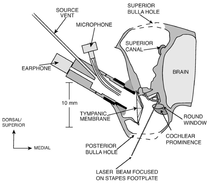
A schematic of a coronal section through the chinchilla ear illustrating: accesses to the middle ear through the two surgically produced bulla holes, the placement of the earphone and the laser focused on the stapes footplate.
A hole was then introduced into the posterior bulla to visualize the round window and the lenticular process of the incus. Both the superior and posterior bullar holes were left wide open (open cavity) throughout the measurements. The bony wall to which the stapedius tendon attaches was then resected between the tendon attachment, the horizontal canal, and the round window in order to visualize the stapes footplate and crura. Three to six reflective beads (each 50 μm in diameter) were then placed on the stapes footplate. Any fluid accumulated in or around the footplate was removed using fine absorbent paper points prior to measurement of the stapes velocity using laser-Doppler vibrometry (LDV).
The pinna and cartilaginous ear canal were resected and the bony ear canal shortened. A probe-tube microphone and calibrated sound source were coupled to the ear canal via a short brass tube that was cemented into the remnant of the bony ear canal. A broadband stimulus with a low-frequency emphasis (log chirp) with frequency components at 11 Hz intervals between 11 Hz and 24 Hz was used as the stimulus. The limited high-frequency output of our sound source restricted the usable frequency range to below 8000 Hz. At frequencies below 100 Hz noise became a problem, especially in the laser measurements. Both the sound pressure at the tympanic membrane (PTM) and the stapes velocity (Vs) were measured in response to log-chirp stimuli at three levels (covering a 20 dB range from 74 to 94 dB SPL) to check for repeatability and linearity. Minor deviations in linearity were observed near 160 Hz. These deviations are consistent with previous work (Ruggero et al., 1996; Rosowski et al., 2006; Songer and Rosowski, 2006) and are usually attributed to an inner ear nonlinearity.
After a series of base line measurements, the cochlea was drained by creating a large hole (0.5 mm×1.0 mm) in the bony cochlear prominence near the round window (Fig. 1) and then using paper points to remove fluid from the cochlea. After draining the cochlea, the round window was perforated in order to ensure continued drainage. In some animals a hole in the superior semicircular canal was introduced prior to creating the hole in the cochlear prominence. After the cochlea was drained, the middle-ear input admittance (YME) and middle-ear transfer function (Hp) were measured repeatedly to test for preparation stability.
The stapes footplate was then fixed by applying either dental cement or Superglue gel ®, forming a connection between the stapes and the adjacent petrous bone. The cement or glue was allowed to dry for at least 10 min. After the glue had hardened, a series of measurements of YME were made. Hp measurements were not possible after fixation because the glue covered the stapes footplate, which was the former location of the reflectors used for measurements of Vs. In two cases new reflectors were placed either on the glue fixing the footplate or on the crus of the stapes to estimate Vs after fixation. To evaluate the effectiveness of the fixation we also measured the cochlear potential at the round window using a silver wire electrode both before and after fixation in three ears using procedures described previously (Songer and Rosowski, 2005). We were also able to compare our measurements of the magnitude of the admittance with the stapes fixed in these ears to that measured in ears in which the inner ear was drained prior to fixation and demonstrate that after fixation the state of the fluid in the inner ear does not impact our measurements of .
B. Instrumentation
1. Source and admittance measurements
The sound stimulus and instrumentation used have been described previously (Songer and Rosowski, 2005, 2006) but will be summarized here. The stimulus we used was a train of 100 log chirps with frequency components between 11 Hz and 24 kHz. The stimulus was generated with a series of LabView scripts and presented to the ear with a hearing-aid earphone (Knowles ED-1913) that was part of a sound-source/measurement assembly with a high acoustic output impedance (Ravicz et al., 1992; Rosowski et al., 2006). A hearing-aid microphone (Knowles EK-3027) was built into the sound source/measurement assembly and used to measure the resultant sound pressure in the ear canal.
The microphone data recorded at the tympanic membrane in conjunction with the Norton equivalent of the source were utilized to calculate the middle-ear input admittance (YME). The Norton equivalent of the acoustic source was determined using previously described procedures (Songer and Rosowski, 2006; Lynch et al., 1994) where the response of the sound source is characterized using a series of acoustic loads of known impedance. To determine YME, the volume velocity of the Norton equivalent representation of the sound source (Usrc) was divided by the sound pressure at the tympanic membrane (PTM) and then the equivalent admittance of the source (Ysrc) was subtracted from the total admittance
| (1) |
The admittance was then corrected for the residual ear canal and earphone-coupler space using a transmission-line correction (Lynch et al., 1994; Voss and Shera, 2004) where the length of the residual canal and sound coupler was estimated to be 6.0 mm and the radius of the tube was 2.4 mm (Songer and Rosowski, 2006).
2. Stapes velocity measurements
Laser-Doppler vibrometry (LDV) was used to detect the sound-induced stapes velocity (Vs) based on the Doppler shift of the light reflected from glass beads placed on the stapes footplate according to a previously described procedure (Songer and Rosowski, 2006). We used a single point LDV from Polytech PI (OFV 5000) to measure Vs. The voltage output from the vibrometer is proportional to the velocity of the moving object and the sensitivity of the LDV system was determined through comparison with a reference accelerometer. A micromanipulator was used to focus and direct the laser light on the stapes footplate. The approximate measurement angle was between 50 and 60° relative to horizontal. No corrections for the angle were performed. Where necessary, Vs was converted to a volume velocity (Us) by multiplying it by the nominal area of the stapes footplate (As =1.98 mm2 (Vrettakos et al., 1988)).1
The middle-ear transfer function was defined as where Vs was measured as described above and PTM is the pressure measured in the ear canal and was calculated from the microphone voltage recorded in the ear canal, and converted to Pascals using a previous calibration performed against a reference microphone
All of the data presented in this paper were normalized for measurement system gains and attenuations (Songer and Rosowski, 2005, 2006). Measurements of microphone voltage and stapes velocity were made for stimulus levels of 74, 84, and 94 dB SPL in each ear and in each condition, except for the stapes fixed condition in which velocity measurements were not possible. Over the majority of the frequency range described here (100–8000 Hz) both the microphone signal and the laser signal were generally linear with a signal that exceeded the noise floor by at least 10 dB.
III. DEFINITION OF TRANSMISSION MATRIX ELEMENTS
A. Matrix in the normal ear
The transmission matrix (T) we use to describe the middle ear is illustrated in Fig. 2, and defined by Eq. (2) where PTM is the pressure at the tympanic membrane, UTM is the volume velocity of the tympanic membrane, PO is the sound pressure produced by the middle ear at its output, and US is the stapes volume velocity. In the normal condition PO is equivalent to the sound pressure within the cochlear vestibule, PV. We have defined both the volume velocity going into the middle ear (UTM) and the stapes volume velocity (US) leaving the two port as positive (Fig. 2). The transmission matrix elements A, B, C, and D are four complex matrix elements that can be used to characterize the relationship between the variables at the ports, i.e.
FIG. 2.
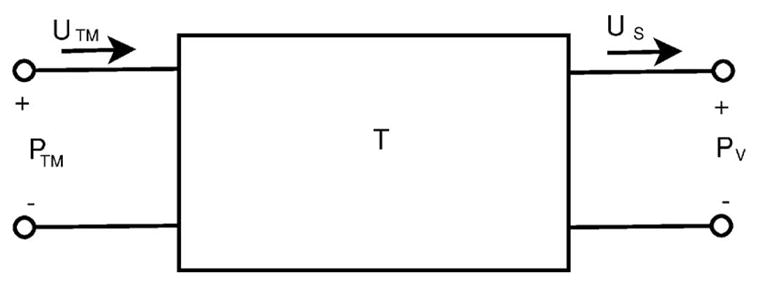
The mechano-acoustic two-port network used to describe the middle ear of the chinchilla. PTM is the sound pressure at the tympanic membrane, UTM is the volume velocity of the tympanic membrane, PV is the sound pressure in the vestibule (and equal to PO in the normal condition), and US is the stapes volume velocity. T represents the transmission matrix with matrix elements of A, B, C, and D.
| (2) |
In the matrix equation above, we can directly measure three of the four input/output variables: PTM, UTM and US.
B. Matrix with the cochlea drained
We assume that by draining the cochlea, we reduce the pressure on the medial side of the stapes to zero, thereby setting PO to zero and simplifying the matrix to Eq. (3), where , and are response variables measured with the cochlea drained:
| (3) |
Determining the resultant equations for PTM and UTM allows us to solve for both B and D in terms of the measured quantities: and , where the superscript D marks values measured with the cochlea drained, and the area of the stapes footplate (As)
| (4) |
| (5) |
C. Matrix with fixed stapes
By fixing the stapes with cement we are able to greatly diminish |US|. If we assume that the resulting stapes velocity is negligible compared to the normal velocity, Eq. (2) reduces to Eq. (6) where the superscript F denotes measured response variables after fixation
| (6) |
where is the effective middle-ear output pressure acting on the fixed stapes, and is equivalent to the pressure acting on a rigid inner-ear load. Equation (6) leads us to equations for both A and C
| (7) |
| (8) |
Since we do not measure directly, we can calculate the relationship between A and C as
| (9) |
Using Eqs. (4), (5), and (7) as well as the reciprocity theorem, we can calculate the fourth matrix parameter (Shera and Zweig, 1992). The reciprocity theorem states that in any passive linear network the forward transfer admittance is equal to the reverse transfer admittance or, in the case of our network representation,
| (10) |
Assuming reciprocity, we can solve for C independently of A and PO as demonstrated in Eq. (11)
| (11) |
D. Definition of transfer matrix and load impedances
Using our measurements of YME and Hp in conjunction with calculations of the transmission matrix parameters and the impedance of our source, we can calculate the cochlear input impedance (Zc), the middle-ear input impedance ( ) and the middle-ear output impedance (Zout).
Zc is the load on the middle ear in the intact state. Using the transmission matrix as well as our measurements of YME and Hp we can solve for Zc.2
| (12) |
In addition to determining ZME from our measurements of YME, we can also calculate ZME using the matrix in Eq. (2) as demonstrated in Eq. (13)
| (13) |
Zout is equal to PO/US in the reverse direction and describes the load the middle ear would place on a sound source in the inner ear. Zout is calculated using the two-port model with the input port loaded by the ear canal and the earphone impedances (the impedance of the sound source within the ear). This load is denoted as Zsrc (Songer and Rosowski, 2006) and the equation for Zout follows:
| (14) |
IV. RESULTS OF THE PHYSIOLOGICAL MEASUREMENTS
Data were collected from eight ears. In three of the ears, draining the cochlea led to significant fluid accumulation in the oval-window niche, occluding our reflectors and preventing us from obtaining stapes-velocity data. The data used to calculate the transmission matrix parameters are from the five ears in which we were able to successfully make measurements in all three experimental conditions: 1) TM, ossicles and cochlea intact, 2) cochlea drained, and 3) stapes fixed.
To compare our measurements to previous results, the data are presented in terms of transfer functions: the middle-ear input admittance (YME= UTM/PTM) and the middle-ear transfer function (Hp = VS/PTM).
A. Normal ear YTM and Hp
The data from five ears were acquired in the intact state. The mean magnitude and phase of YME for the normal ear is illustrated in Fig. 3. This mean result is similar to other measurements of YME with open middle-ear spaces (Songer and Rosowski, 2006; Rosowski et al., 2006) and is presented with units of acoustic Siemens (1S=1m3-s−1-Pa−1).
FIG. 3.
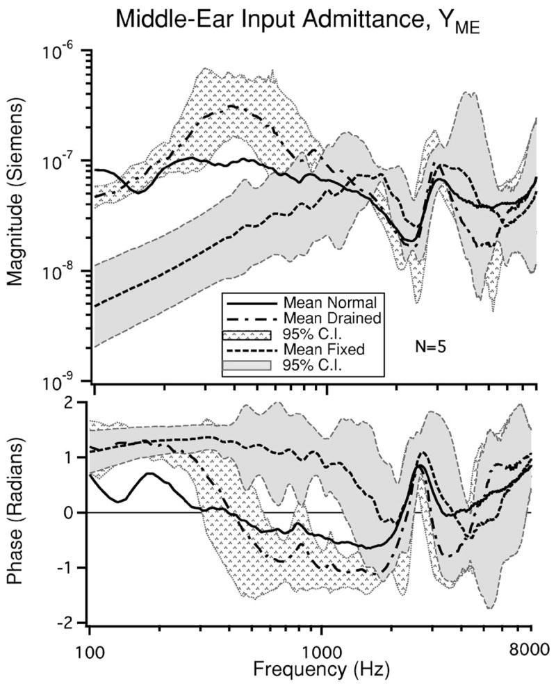
The mean magnitude and phase of YME for each condition: normal (intact), cochlea drained, and stapes fixed (N=5). The 95% confidence intervals (C.I.s) are shown for both the drained and stapes fixed conditions. Figure 8 shows the 95% C.I. for YME the intact condition.
There are three prominent features in the mean |YME| data from the normal or intact ear: a minimum near 160 Hz, a second minimum near 2400 Hz, and a maximum near 3 kHz. These extrema in the YME magnitude are associated with changes in the phase of YME. The prominent features in the mean are present in all five ears, with slight differences in the sharpness of the extrema. Minima in middle-ear transmission near 160 Hz have been observed previously in measurements of YME (Songer and Rosowski, 2006) as well as in measures of cochlear microphonic (Dallos, 1970) and cochlear potential (Songer and Rosowski, 2005). It is hypothesized that these minima are due to the influence of the helicotrema on low-frequency cochlear input impedance (Dallos, 1970; Songer and Rosowski, 2006; Rosowski et al., 2006). The minimum near 2400 Hz is attributed to an antiresonance produced by the open holes in the bulla. Similar minima have been observed previously in chinchilla (Songer and Rosowski, 2006; Rosowski et al., 2006) and other species (Moller, 1965; Guinan and Peake, 1967;Ravicz et al., 1992).
The mean magnitude and phase of the Hp in five intact ears is illustrated in Fig. 4. The frequency response of Hp is similar to the frequency response observed for YME and to previous measurements (Songer and Rosowski, 2006; Ruggero et al., 1990): minima in |Hp| occur at 160 and 2400 Hz and a maximum is apparent near 3000 Hz. The phase is primarily decreasing throughout the frequency range except near 160 Hz, and between 2400 and 3000 Hz where there are phase changes associated with the extrema in the magnitude. Above 5 kHz the phase of Hp decreases more rapidly.
FIG. 4.

The mean magnitude and phase for the Hp measured in each condition. The 95% confidence intervals (C.I.) for both the normal and drained states are also illustrated.
B. Drained cochlea YME and Hp
The mean magnitude and phase as well as the 95% confidence intervals3 for YME after the cochlea has been drained are illustrated in Fig. 3. The mean has a maximum at 400 Hz and a minimum near 2400 Hz. The phase at 100 Hz is near 1 rad and remains nearly constant until approximately 300 Hz, above which there is a rapid phase transition to near −1 rads where it remains until peaking near 2400 Hz. Between 100 and 300 Hz, the upward slope in magnitude and the positive angle between 1 and π/2 radians suggest a stiffness controlled admittance. Between 600 and 2000 Hz, the downward slope in magnitude and the angles between −1 and −π/2 suggest a mass-controlled admittance. The minimum near 2400 Hz is consistent with the open-cavity resonance observed in the normal ear.
The Hp after draining the inner ear has many similarities to . Draining the inner ear results in a mean increase in for frequencies below 1400 Hz (Fig. 4). This increase has a peak near 400 Hz, below which the slope is positive and the phase is between 1 and π/2 rad and above which the slope is negative and the phase is between −1 and −π/2 rad. For frequencies above 1500 Hz there is little difference between the Hp measured in the intact ear and that observed after draining. The minimum near 2400 Hz associated with the open-cavity resonance is still observed. For frequencies above 5 kHz the phase decreases rapidly.
Both and show a low-frequency resonance (peak near 400 Hz with a π change in phase) that is consistent with measurements of middle-ear mechanics associated with cochlear draining (Moller, 1965; Lynch, 1981; Allen, 1986; Puria and Allen, 1998). The appearance of this resonance after cochlear draining is consistent with the removal of cochlear damping (Moller, 1965; Rosowski et al., 2006).
C. Fixed stapes YME and Hp
The mean magnitude and phase of YME after fixing the stapes is illustrated in Fig. 3. For low frequencies, fixing the stapes results in a decrease in |YME| and leads to a phase close to π/2 rad. This change in YME is consistent with previous work (Moller, 1965; Lynch, 1981) that suggests the middle-ear input impedance becomes stiffer as a result of fixation for frequencies below 1000 Hz. The mean increases proportionately with frequency above 100 Hz, reaching a peak near 1500 Hz. The peak is followed by a minimum at 2400 Hz. The phase at 100 Hz is between 1 and 1.5 rad and remains nearly constant until near 1500 Hz above which it rapidly transitions to a value less than 0 rad.
The varies between the five ears (Fig. 5). This variation is likely due to differences in the effectiveness of fixation. The more complete the fixation, the smaller the low-frequency admittance is expected to be. According to this criterion, ear 3 has the most complete fixation of the ears we tested.
FIG. 5.
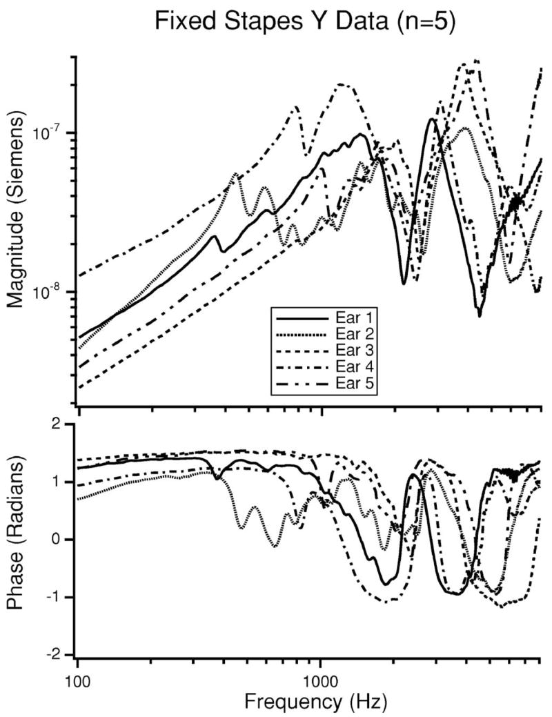
The magnitude and phase of YME after the stapes has been fixed (n=5). Ear 3 has the lowest admittance and is considered to have the best fixation. Note the sharp anti resonance near 2400 Hz which is associated with the open bulla holes in our preparation.
It was not possible to measure Hp after fixation of the stapes because the glue overlapped the location of stapes reflectors. In two cases, we placed additional reflectors on the crus to record the stapes velocity after a partial fixation and observed a 20–25 dB decrease in Hp for frequencies below 500 Hz. Between 500 and 1500 Hz the effect of fixation diminishes and above 1500 Hz, the change in Hp as a result of fixation was less evident.
Since measurements of stapes velocity were not routinely possible after fixation, we also measured the cochlear potential (CP) normalized by PTM(G= CP/PTM) before and after fixation in three ears. The fixation in these ears resulted in a 10–30 dB reduction in G for frequencies below 1500 Hz. Above 2 kHz there was little difference between G before and after fixation. This indicates that our fixation4 is most effective for frequencies below 1500 Hz.
D. Summary of physiological findings
Figure 3 illustrates YME in response to each of the experimental conditions: intact ear, cochlea drained, and stapes fixed. Above 1500 Hz, the difference between the means of the conditions is not significant. This suggests that for frequencies above 1500 Hz the state of the inner ear is not affecting our measurements. For frequencies below 1500 Hz we observe differences in YME both in magnitude and phase in response to our manipulations as described above. In both the intact ear and after the cochlea is drained, Hp (Fig. 4) has a similar frequency dependence to YME.
V. COMPUTATION OF TRANSMISSION MATRIX PARAMETERS
The transmission matrix parameters (A, B, C, and D) are calculated for each of the five ears based on the individual YME and Hp measurements. The mean and 95% confidence intervals of the A, B, C, and D calculations from the five ears are our first estimate of these four parameter values and their variance. Our measurements of both G and Hp after fixation suggest that the assumed large reduction in stapes motion after our fixation procedure is only strictly valid for frequencies below 1500 Hz. Since our estimates of A, C, ZME, Zout, and Zc are dependent on the fixation measurements and this assumption, they are most reliable for frequencies below 1500 Hz.
A. Two-port description as transmission matrix
B and D are calculated from measurements taken after the cochlea is drained. B is the ratio of the drained PTM to drained US and has units of Pa s m−3. The mean value of our five estimates of B along with the 95% confidence intervals are illustrated in Fig. 6(B). The most prominent feature of |B| is a broad minimum near 350 Hz which is associated with a transition in phase from near −π/2 to near π/2. As discussed earlier, this minimum is related to a middle-ear resonance that is observed when the cochlear damping is removed.
FIG. 6.
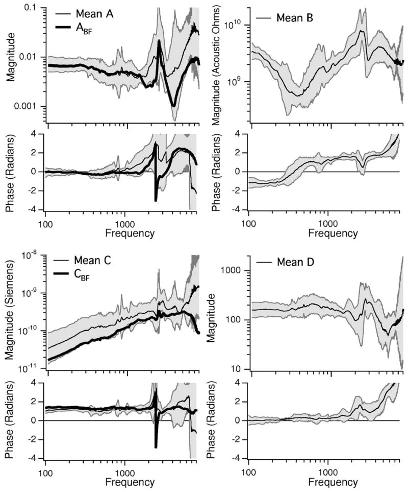
The mean values of the transmission parameters (A, B, C, and D) along with the 95% confidence intervals estimated from five ears. The mean A and C are plotted as well as the parameters calculated from the best fixation measurements, Abf and Cbf. The calculations of B and D do not depend on fixation, therefore only the mean and C.I.s are illustrated.
D is the ratio of the drained UTM to the drained US and is dimensionless. The mean value of the five estimates of D is illustrated in Fig. 6(D) along with the 95% confidence intervals. For frequencies below 1500 Hz the average |D| is about 165, with a phase angle near zero. There is a peak in the average |D| near 3 kHz with a value of 250, with a phase angle at the peak of about π/2. At higher frequencies |D| decreases and the phase angle grows.
The transmission parameters A and C are calculated using B and D as well as measurements taken after fixing the stapes. C is defined in Eq. (11) and has units of admittance (m3-s−1-Pa−1). The mean and 95% confidence intervals of the five individual C computations are illustrated in Fig. 6(C). |C| is roughly proportional to frequency and the phase angle of C is near π/2 over the majority of the frequency range. C was also calculated using the measurements from the fixation that produced the largest reduction in |YME| (ear 3) and the mean B and D. We refer to this estimate as Cbf, where the bf stands for the “best fixation.” The Cbf calculation is intended to reduce the effect of potential procedural problems (ineffective fixation) on model predictions and results. |Cbf| is about 60% of the mean |C| across the entire frequency range. At 2500 Hz there is a phase discontinuity in Cbf due to residual effects of the sharp bulla-hole-cavity anti resonance observed in the stapes-fixed data from ear 3 (Fig. 5).
A is unitless and calculated using Eq. (7) and Eq. (9). The mean and 95% confidence intervals of the five individual estimates of A are illustrated in Fig. 6(A). Below 1500 Hz, A is fairly constant with a magnitude near 0.007, a phase near zero and is approximately 1/D. Above 1500 Hz, there is an increase in both the magnitude and phase of A. Due to the variable quality of our fixations for frequencies above 1500 Hz, we also calculated Abf using the best fixation measurements of ear 3 (also plotted in Fig. 6(A)). For frequencies below 1500 Hz both A and Abf are nearly identical. Above 1500 Hz, however, |Abf| is smaller than |A|, has a more prominent peak near 2500 Hz and a phase discontinuity at the same frequency. The sharp phase transition in Abf near 2500 Hz can again be attributed to a strong cavity anti resonance observed in the fixed-stapes data from ear 3 (Fig. 5).
B. Cochlear input impedance
The mean and 95% confidence interval of the five Zc estimates calculated using Eq. (12) are illustrated in Fig. 7. The magnitude and phase are relatively constant with frequency. The Zc calculated from the best fixation, , is also illustrated. One feature of our calculation of Zc is a peak near 160 Hz and an associated change in phase. This peak occurs at the same frequency as the observed minimum in |YME|. The minimum in |YME| has been attributed to the effect of the helicotrema in previous studies (Songer and Rosowski, 2006; Dallos, 1970).
FIG. 7.
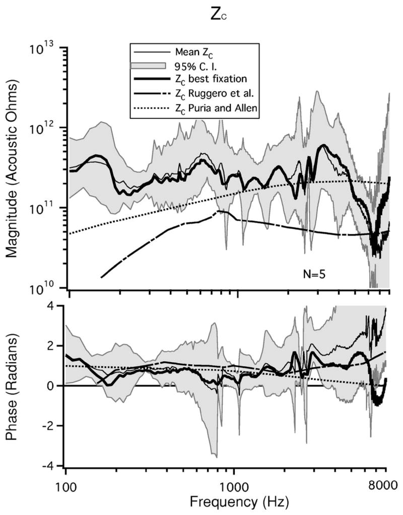
The mean calculated Zc(n=5) with 95% confidence intervals. , the Zc calculated from the best fixation, as well as Zc estimated by Ruggero et al. (1990) and Puria and Allen (1991) are also illustrated.
Calculations of Zc presented by Ruggero et al. (Ruggero et al., 1990) and Puria and Allen (Puria and Allen, 1991) are also illustrated in Fig. 7. Our calculations of Zc differ from those presented by Ruggero in three major aspects: 1) our estimate has a magnitude that is 3–4 times larger than that of Ruggero et al., 2) our measurements do not exhibit the low-frequency roll off observed in the Ruggero et al. estimates and 3) our measurements have much more fine structure. The Puria and Allen estimates of Zc have a magnitude that is generally similar to our estimate of Zc, especially at frequencies between 1000 and 5000 Hz. The Puria and Allen estimates have a low-frequency roll off that is slower than that seen in the Ruggero et al. estimates but still suggest lower impedance magnitude than our estimates at frequencies less than 800 Hz. The three estimates of the phase of Zc are similar, with the largest differences observed at the highest and lowest frequencies.
C. Calculations of YME, Hp and middle-ear output impedance
The mean of the YME calculated from the five individual sets of impedance parameter estimates ( Eq. (13)) and the YME calculated from Abf, Cbf, Zbf and the mean A and B are compared to the 95% confidence intervals from our measurements of YME in Fig. 8. The magnitude and phase of the two computations and our measurement of YME show excellent agreement for frequencies between 100 Hz and 6 kHz, thereby demonstrating self-consistency within the calculations. The YME calculated with the best fixation measurement, shows some differences from the measurements and the other estimate at frequencies above 6 kHz.
FIG. 8.
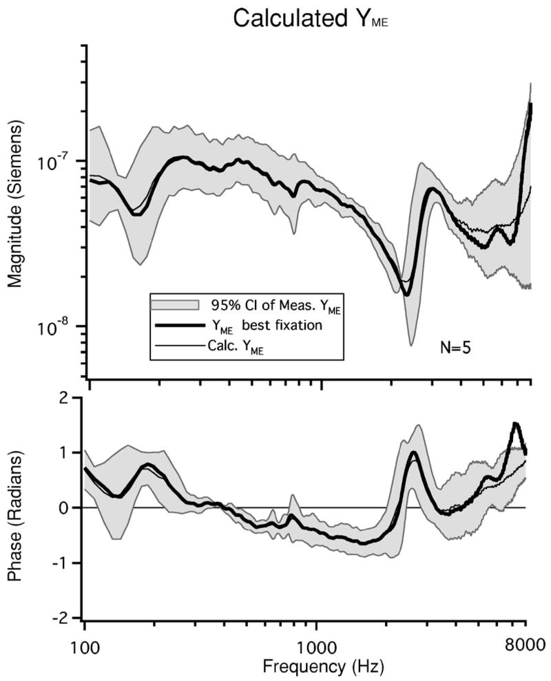
The 95% confidence intervals of the measured YME data as well as the mean calculated YME and the are illustrated. Both calculations of YME are within the 95% C.I. of the measurement data for frequencies below 6 kHz.
A second consistency test is to compare our calculated middle-ear transfer function (Hp) to the measured values of Hp as illustrated in Fig. 9. The calculations of Hp are a good fit to the data, however, for frequencies above 2 kHz, the calculation of Hp using the best fixation measurement is closer in magnitude and phase to the measured data. Thus, our calculations of both YME and Hp suggest that our transmission matrix parameter values are internally consistent. A slight improvement in agreement between the measured and predicted values is achieved at high frequencies using parameters calculated based on the best fixation measurements, however the YME estimated with the best-fixation data differs slightly from the mean estimates above 6 kHz.
FIG. 9.

The 95% confidence intervals of the measured Hp, the mean calculated Hp, and the . The data have a better fit to the measured Hp data at high frequencies.
The mean calculated Zout along with the 95% confidence intervals are illustrated in Fig. 10. Zout has a magnitude that is inversely proportional to frequency and a phase near π/2 for frequencies below 1 kHz. This is consistent with Zout being compliance dominated within this frequency range. Zout is dependent on the impedance of the sound source (Zsrc) as well the ear canal since they make up the load on the middle ear in the reverse direction (from the oval window). The relationship between Zout and Zsrc is explicitly stated in Eq. (14) and Zsrc is illustrated in Fig. 10. For frequencies below 2400 Hz, Zout generally appears to be a scaled version of Zsrc where the mean scaling factor between 100 and 8000 Hz is 82 dB.
FIG. 10.
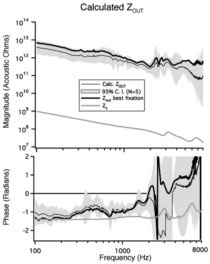
The mean calculated Zout with 95% confidence intervals as well as . Zsrc (Zs) is also illustrated.
The Zout calculated from the best fixation measurement ( is also plotted. is larger than |Zout| over the entire frequency range. The phase of has some rapid phase cycling near 2400 Hz that is associated with a strong antiresonance in the original measurements. Since Zout is a driving-point impedance and the middle-ear is a passive system, we expect the angle of Zout to vary between ±π/2. However, artifact in the handling of the phase data associated with small changes in the cavity resonance near 2400 Hz causes the angle to exceed these bounds at some frequencies above 2400 Hz.
VI. DISCUSSION OF MODEL ESTIMATES OF NORMAL EAR FUNCTION
A. Comparison to other Zc estimates
Both Ruggero et al. (Ruggero et al., 1990) and Puria and Allen (Puria and Allen, 1991) report values of Zc in chinchilla. The Zc estimate published by Ruggero et al. (Ruggero et al., 1990) was calculated based on measurements of Vs and previously published measurements of PV. Between 200 and 2000 Hz our estimate of Zc is, on average, 11.6 dB (3.8 times) greater than that published by Ruggero et al. Puria and Allen use a spatially varying transmission line model together with measurements of the dimensions of scala vestibuli and scala tympani to estimate the value of Zc (Puria and Allen, 1991) and arrive at a value of Zc that is similar to our estimate at frequencies between 1000 and 5000 Hz, and as much as 12.9 dB (4.4 times) greater than that reported by Ruggero et al. For frequencies between 400 Hz and 2 kHz the three estimates of Zc, though they differ in magnitude, exhibit similar frequency responses both in magnitude and phase. One factor that would reduce the magnitude of our estimate of Zc by 4–6 dB (1.6–2 times), would be if we used a correction for the angle of our observed stapes motion. The stapes velocities in our study were measured with an approximate angle of 50–60° between our laser and the axis of “piston-like” motion of the stapes. The cosine of these angles describes the error in estimating the piston-like motion. However, given that the motion of the stapes in humans, cats, and gerbils (Decraemer and Khanna, 2004) and probably chinchilla becomes complicated at frequencies above a few kHz, such a correction is problematic (Chien et al., 2006).
While the Puria and Allen Zc model does suggest a decrease in Zc magnitude above 2 kHz, the minimum they compute is at 15 kHz instead of the minima between 6 and 8 kHz that we observe. The phase above 3 kHz that we predict from the transmission matrix analysis is similar to that reported by Ruggero et al. Below 500 Hz the data from Ruggero et al. exhibit a positive slope of 7 dB/octave, whereas our estimates suggest a relatively flat frequency response in this range.
B. Utility of Zout estimates
The transmission matrix analysis of the middle ear allows us to estimate Zout for the normal chinchilla ear in addition to ZME and Zc. Zout has been calculated using similar methodologies in human cadaveric temporal bones (Puria, 2003). The Zout in human temporal bones (Puria, 2003) exhibits a similar frequency dependence to that presented here but with a magnitude of 1010 mks ohms near 2 kHz (Puria, 2003), which is two orders of magnitude lower than our estimated chinchilla Zout. A potential difference between the measurements made in this study and the observations in temporal bones could be from the acoustic source. Zout can be strongly affected by the impedance of the sound source in the ear canal (Voss and Shera, 2004).
Measurements of Zc in conjunction with measurements of Zout can be used to estimate the stapes reflection coefficient (Puria, 2003) and the round-trip middle-ear gain (Voss and Shera, 2004) to provide further insight into otoacoustic emission (OAE) generation mechanisms. In addition to the utility of calculations of Zout in improving our understanding of OAEs, our calculated measurements of Zout in chinchilla can be used to develop a better understanding of the middle-ear load on the inner ear in response to bone-conducted sound stimuli (Songer, 2006).
C. Benefits and limitations of transmission matrix characterization of the middle ear
Transmission matrix analysis has been used to describe the middle ears of cats (Voss and Shera, 2004) as well as human cadaveric temporal bones (Puria, 2003). The transmission matrix characterization of the chinchilla middle ear reported here has many similarities to those reported previously, but differs in some aspects. In this report we did not rely on driving the middle ear “in reverse” with OAEs. Instead, we focused on the forward transmission of the middle ear. This led us to use fixation as one of our experimental conditions. As discussed previously, the degree of fixation varied between ears (Fig. 5) and was most effective at frequencies less than 1.5 kHz. Despite these drawbacks, the predicted values of Zc and Zout appear reasonable in terms of their frequency dependence. Additional tests of the high-frequency (>1500 Hz) characteristics of the chinchilla middle-ear two port will be useful in applications where the high-frequency responses of the middle ear are critically important and can be implemented by directly measuring the pressure in the vestibule instead of relying on measurements of stapes fixation. However, cases where the low-frequency responses are of greatest interest, such as superior canal dehiscence syndrome (Songer and Rosowski, 2007), will benefit from the existing transmission matrix analysis.
The transmission matrix characterization of the middle ear makes no assumptions about the load on either side of the middle ear and can be used in a wide variety of applications ranging from developing models of disease (e.g., superior semicircular canal dehiscence) to improving our understanding of OAEs.
Acknowledgments
This work has been supported by a NSF graduate student fellowship, NIH training grant, and additional NIH grants. S.N. Merchant, C.A. Shera, W.T. Peake, and M.E. Ravicz provided insights and suggestions. M.L. Wood assisted with data collection and animal surgery.
Footnotes
As discussed later, this simple conversion to volume velocity assumes that the piston-like component of stapes motion dominates the single-point measurement we make. When this assumption was tested in cats and human temporal bones (Heiland et al., 1999; Hato et al., 2003; Decraemer and Khanna, 2004; Chien et al., 2006; Voss et al., 2000) it was generally found to be valid for frequencies less than 2 kHz and somewhat questionable at higher frequencies.
Zc can be solved for in two additional ways as illustrated below; however, our calculations of Zc are made using Eq. (12) because these values were empirically determined to be the most stable and repeatable:
The 95% confidence interval (C.I.) can be defined as 1.96 times the standard error and indicates the probability (p<0.05) that the actual mean is within the specified range.
We have demonstrated that, despite our application of Superglue to the stapes footplate and surrounding bone, we were unable to create a complete fixation of the stapes. However, in order to maintain a simple nomenclature we continue to refer to this process as fixation and as data with a “fixed stapes.”
Contributor Information
Jocelyn E. Songer, Eaton-Peabody Laboratory of Auditory Physiology, Massachusetts Eye and Ear Infirmary, 243 Charles St., Boston, Massachusetts 02114 and Speech and Hearing Bioscience and Technology, Health Sciences and Technology, Harvard-MIT, Cambridge, Massachusetts 02138.
John J. Rosowski, Eaton-Peabody Laboratory of Auditory Physiology, Massachusetts Eye and Ear Infirmary, 243 Charles St., Boston, Massachusetts 02114, Speech and Hearing Bioscience and Technology, Health Sciences and Technology, Harvard-MIT, Cambridge, Massachusetts 02138 and Department of Otology and Laryngology, Harvard Medical School, Boston, MA 02114
References
- Allen JB. Measurements of eardrum acoustic impedance. In: Allen JB, Hall JH, Hubbard A, Nealy ST, Tubis A, editors. Peripheral Auditory Mechanisms. Springer-Verlag; New York: 1986. pp. 44–51. [Google Scholar]
- Chien W, Ravicz ME, Merchant SN, Rosowski JJ. The effect of methodological differences in the measurement of stapes motion in live and cadaver ears. Audiol Neuro-Otol. 2006;11:183–197. doi: 10.1159/000091815. [DOI] [PMC free article] [PubMed] [Google Scholar]
- Dallos P. Low-frequency auditory characteristics: Species dependence. J Acoust Soc Am. 1970;48(2):489–499. doi: 10.1121/1.1912163. [DOI] [PubMed] [Google Scholar]
- Decraemer WF, Khanna SM. Measurement, visualization and quantitative, analysis of complete three-dimensional kinematical data sets of human and cat middle ear. In: Gyo K, Wada H, Hato H, Koike T, editors. The Proceedings of the Third International Symposium on Middle Ear Research and Oto-Surgery. World Scientific; Singapore: 2004. pp. 3–10. [Google Scholar]
- Desoer CA, Kuh ES. Basic Circuit Theory. McGraw-Hill; New York: 1969. [Google Scholar]
- Gan RZ, Sun Q, Dyer RK, Jr, Chang KH, Dormer KJ. Three-dimensional modeling of middle-ear biomechanics and its applications. Otol Neurotol. 2002;23:271–280. doi: 10.1097/00129492-200205000-00008. [DOI] [PubMed] [Google Scholar]
- Goode RL, Killion M, Nakamura K, Nishihara S. New knowledge about the function of the human middle ear: Development of an improved analog model. Am J Otol. 1994;15:145–154. [PubMed] [Google Scholar]
- Guinan JJ, Jr, Peake WT. Middle-ear characteristics of anesthetized cats. J Acoust Soc Am. 1967;41(5):1237–1261. doi: 10.1121/1.1910465. [DOI] [PubMed] [Google Scholar]
- Hato N, Stenfelt S, Goode RL. Three-dimensional stapes footplate motion in human temporal bones. Audiol Neuro-Otol. 2003;8(3):140–152. doi: 10.1159/000069475. [DOI] [PubMed] [Google Scholar]
- Heiland KE, Asai RL, Huber AM. A human temporal bone study of stapes footplate movement. Am J Otol. 1999;20:81–86. [PubMed] [Google Scholar]
- Koike T, Wada H, Kobayashi T. Modeling of the human middle ear using the finite-element method. J Acoust Soc Am. 2002;111(3):1306–l317. doi: 10.1121/1.1451073. [DOI] [PubMed] [Google Scholar]
- Kringlebotn M. Network model for the human middle ear. Scand Audiol. 1988;17:75–85. doi: 10.3109/01050398809070695. [DOI] [PubMed] [Google Scholar]
- Ladak J, Funnell WRJ. Finite-element modeling of the normal and surgically repaired cat middle ear. J Acoust Soc Am. 1996;100(2):933–944. doi: 10.1121/1.416205. [DOI] [PubMed] [Google Scholar]
- Lynch TJ., III . Signal Processing by the Cat Middle Ear: Admittance, and Transmission, Measurements and Models Doctoral thesis. Massachusetts Institute of Technology; 1981. [Google Scholar]
- Lynch TJ, III, Peake WT, Rosowski JJ. Measurements of the acoustic input impedance of cat ears: 10 Hz–20 Khz. J Acoust Soc Am. 1994;96(4):2184–2209. doi: 10.1121/1.410160. [DOI] [PubMed] [Google Scholar]
- Miller JD. Audibility curve of the chinchilla. J Acoust Soc Am. 1970;48(2):513–523. doi: 10.1121/1.1912166. [DOI] [PubMed] [Google Scholar]
- Moller AR. An experimental study of the acoustic impedance of the middle ear and its transmission properties. Acta Oto-Laryngol. 1965;60:129–149. doi: 10.3109/00016486509126996. [DOI] [PubMed] [Google Scholar]
- Nedzelnitsky V. Sound pressures in the basal turn of the cat cochlea. J Acoust Soc Am. 1980;68:1676–1689. doi: 10.1121/1.385200. [DOI] [PubMed] [Google Scholar]
- Peake WT, Rosowski JJ, Lynch TJ., III Middle-ear transmission: Acoustic versus ossicular coupling in cat and human. Hear Res. 1992;57:245–268. doi: 10.1016/0378-5955(92)90155-g. [DOI] [PubMed] [Google Scholar]
- Puria S. Measurements of human middle ear forward and reverse acoustics: Implications for otoacoustic emissions. J Acoust Soc Am. 2003;113(5):2773–2789. doi: 10.1121/1.1564018. [DOI] [PubMed] [Google Scholar]
- Puria S. Middle-ear two-port measurements in human cadaveric temporal bones: Comparison with models. In: Gyo K, Wada H, Hato H, Koike T, editors. The Proceedings of the Third International Symposium on Middle Ear Research and Oto-Surgery. World Scientific; Singapore: 2004. pp. 43–50. [Google Scholar]
- Puria S, Allen JB. A parametric study of cochlear input impedance. J Acoust Soc Am. 1991;89(1):287–309. doi: 10.1121/1.400675. [DOI] [PubMed] [Google Scholar]
- Puria S, Allen JB. Measurements and model of the cat middle ear: Evidence of tympanic membrane acoustic delay. J Acoust Soc Am. 1998;104:3463–3481. doi: 10.1121/1.423930. [DOI] [PubMed] [Google Scholar]
- Ravicz ME, Rosowski JJ, Voigt H. Sound-power collection by the auditory periphery of the mongolian gerbil meriones unguiculatus: I. middle-ear input impedance. J Acoust Soc Am. 1992;92(1):157–177. doi: 10.1121/1.404280. [DOI] [PubMed] [Google Scholar]
- Rosowski JJ, Ravicz ME, Songer JE. Structures that contribute to middle-ear admittance in chinchilla. J Comp Physiol. 2006;192(12):1287–1311. doi: 10.1007/s00359-006-0159-9. [DOI] [PMC free article] [PubMed] [Google Scholar]
- Ruggero MA, Rich NC, Robles L, Shivapuja BG. Middle-ear response in the chinchilla and its relationship to mechanics at the base of the cochlea. J Acoust Soc Am. 1990;87(4):1612–1629. doi: 10.1121/1.399409. [DOI] [PMC free article] [PubMed] [Google Scholar]
- Ruggero MA, Rich NC, Shivapuja BG, Temchin A. Auditory nerve responses to low-frequency tones: Intensity dependence. Aud Neurosci. 1996;2:159–185. [Google Scholar]
- Shera CA, Zweig G. Middle-ear phenomeonology: The view from the three windows. J Acoust Soc Am. 1992;1992:1356–1370. doi: 10.1121/1.403929. [DOI] [PubMed] [Google Scholar]
- Songer JE. Superior Semicircular Canal Dehiscence: Auditory Mechanisms Doctoral thesis. Massachusetts Institute of Technology; 2006. [Google Scholar]
- Songer JE, Rosowski JJ. The effect of superior canal dehiscence on cochlear potential in response to air-conducted stimuli in chinchilla. Hear Res. 2005;210:53–62. doi: 10.1016/j.heares.2005.07.003. [DOI] [PMC free article] [PubMed] [Google Scholar]
- Songer JE, Rosowski JJ. The effect of superior-canal opening on middle-ear input admittance and air-conducted stapes velocity in chinchilla. J Acoust Soc Am. 2006;120(1):258–269. doi: 10.1121/1.2204356. [DOI] [PMC free article] [PubMed] [Google Scholar]
- Songer JE, Rosowski JJ. A Mechano-Acoustic Model of Superior Canal Dehiscence in Chinchilla. J Acoust Soc Am. 2007;122(2) doi: 10.1121/1.2747158. [DOI] [PMC free article] [PubMed] [Google Scholar]
- Voss SE, Rosowski JJ, Merchant SN, Peake WT. Acoustic responses of the human middle ear. Hear Res. 2000;150(1–2):43–69. doi: 10.1016/s0378-5955(00)00177-5. [DOI] [PubMed] [Google Scholar]
- Voss SE, Shera CA. Simultaneous measurement of middle-ear input impedance and forward/reverse transmission in cat. J Acoust Soc Am. 2004;16(4):2187–2198. doi: 10.1121/1.1785832. [DOI] [PubMed] [Google Scholar]
- Vrettakos PA, Dear SP, Saunders JC. Middle ear structure in the chinchilla: A quantitative study. Am J Otolaryngol. 1988;9:58–67. doi: 10.1016/s0196-0709(88)80009-7. [DOI] [PubMed] [Google Scholar]
- Zwislocki J. Analysis of the middle-ear function, Part I. Input impedance. J Acoust Soc Am. 1962;34(8):1514–1523. [Google Scholar]