A Randomization Test for Controlling Population Stratification in Whole-Genome Association Studies

Abstract

Population stratification can be a serious obstacle in the analysis of genomewide association studies. We propose a method for evaluating the significance of association scores in whole-genome cohorts with stratification. Our approach is a randomization test akin to a standard permutation test. It conditions on the genotype matrix and thus takes into account not only the population structure but also the complex linkage disequilibrium structure of the genome. As we show in simulation experiments, our method achieves higher power and significantly better control over false-positive rates than do existing methods. In addition, it can be easily applied to whole-genome association studies.

One of the principal difficulties in drawing causal inferences from whole-genome case-control association studies is the confounding effect of population structure. Differences in allele frequencies between cases and controls may be due to systematic differences in ancestry rather than to association of genes with disease.^1–8 This issue needs careful attention in forthcoming large-scale association studies, given the lack of knowledge regarding relevant ancestral history throughout the genome and the need to aggregate across many individuals to achieve high levels of discriminatory power when many markers are screened.

Existing methods for controlling for population stratification make a number of simplifying assumptions. “Genomic control” is a widely used method that views the problem as one of overdispersion and attempts to estimate the amount by which association scores are inflated by the overdispersion.^9,10 An assumption of this method is that the overdispersion is constant throughout the region being tested. This assumption seems ill advised in large-scale studies of heterogeneous regions; indeed, when the assumption is wrong, it can lead to a loss of power and a loss of control over the test level.⁸ EIGENSTRAT is a recent proposal that computes principal components of the genotype matrix and adjusts genotype and disease vectors by their projections on the principal components.⁸ The assumption in this case is that linear projections suffice to correct for the effect of stratification; the simulation results that we present below put this assumption in doubt. Yu and colleagues¹¹ presented a unified mixed linear model to correct for stratification. Similar to EIGENSTRAT, their model assumes linearity, but it also accounts for multiple levels of relatedness. Finally, “structured association” refers to a model-based approach in which Bayesian methods are used to infer subpopulations and association statistics are then computed within inferred subpopulations.^12,13 The assumptions in this approach inhere in the choice of probabilistic model and in the thresholding of posterior probabilities to assign individuals to subpopulations. This approach is highly intensive computationally, limiting the range of data sets to which it can be applied.

Correcting for stratification is challenging, even if the population structure is known. One may treat the population structure as an additional covariate of the association test. However, in contrast to other covariates, such as age and sex, the genotype information strongly depends on the population structure. Therefore, even if the population structure is known, correcting its confounding effect must take into account this dependency. To exemplify this problematic issue, consider EIGENSTRAT, which uses the axes of variation as covariates (which represent population structure) in a multilinear regression. In some instances, we show that EIGENSTRAT accurately finds the population structure but still fails to correct its effect properly. This happens not because the population structure was inferred incorrectly but because the multilinear regression assumptions do not hold (see the “Discussion” section and appendix A).

An alternative to existing methods is to consider randomization tests (e.g., permutation tests); these are conditional frequentist tests that attempt to compute P values directly by resampling from an appropriate conditional probability distribution and by counting the fraction of resampled scores that are larger than the observed score. On the one hand, randomization tests seem well matched to the stratification problem. Rather than working with individual association scores that require a subsequent familywise correction, we can directly control the statistic of interest (generally, the maximum of association scores across markers). Moreover, by working conditionally, the randomization approach can take into account possible dependencies (linkage disequilibrium [LD]) among markers, an important issue not addressed directly by existing methods. On the other hand, the computational demands of randomization tests can be quite high and would seem to be prohibitively high in large-scale association studies.

Even if the computational issues can be surmounted, performing a standard permutation test with population stratification is not straightforward. The main difficulty is that the null model of the standard permutation test assumes that each one of the individuals is equally likely to have the disease. This assumption could lead to spurious associations when population structure exists.¹⁴ Consider a data set that contains two different populations, each with different prevalences of the disease. Consider further that the population to which each individual belongs is known. In this case, a test for association mapping cannot assume a null model in which the probability of having the disease is equal for all individuals. Rather, the probability of each permutation should be weighted differently, according to the population structure.

In this article, we show how to perform a randomization test that takes into account the population structure. Our method—which we refer to as the “population stratification association test” (PSAT)—works as follows. We assume that a baseline estimate is available for the probability that each individual has the disease, independent of their genotype. This can be obtained from any method that estimates population structure, including STRUCTURE¹² or EIGENSTRAT,⁸; for computational efficiency, we used EIGENSTRAT for the results we report here. We refer to the vector of these estimates as the “baseline probability vector.” We then consider a null hypothesis in which each of the individuals has the disease independently according to the corresponding component of the baseline probability vector. Conceptually, we then resample disease vectors under this null model and, for each sample, compute a statistic (e.g., the association score of the most associated marker). Note that this process is based on the resampled disease vector and the original genotype matrix—that is, we work conditionally on the observed genotypes. The P value is then estimated as the fraction of resampled statistics that are larger than the observed statistic.

Our simulations show that PSAT achieves higher power than that of existing methods. In simulated panels of 1,000 cases and 1,000 controls, PSAT yielded an advantage of up to 14% in power, compared with EIGENSTRAT. An even larger difference was observed between PSAT and genomic control. In addition, PSAT has significantly better control over false-positive rates. When population stratification exists, PSAT maintains a constant false-positive rate, compared with the relatively high (up to 1) false-positive rates of the other methods.

Performed naively, the computation underlying PSAT would be feasible in general only for small problems. As we show, however, the combination of importance sampling and dynamic programming renders PSAT quite feasible for typical whole-genome studies. In a study involving 500,000 SNPs and 1,000 cases and 1,000 controls, we compute a P value in a few minutes.

PSAT is similar in spirit to the method of Kimmel and Shamir,¹⁵ but the algorithmic methodology is quite different; here, as opposed to in the work of Kimmel and Shamir,¹⁵ each of the samplings is weighted differently according to the population structure. This renders the methodology employed by Kimmel and Shamir¹⁵—uniform sampling from the set of permutations induced by a fixed contingency table—inapplicable to the population substructure problem. To solve this problem, we have had to develop a new technique based on a dynamic programming recursion across individuals. This technique makes it possible to efficiently sample disease vectors via importance sampling.

Methods

Definitions

Let M be the number of individuals tested and N be the number of markers. The M×N genotype matrix is denoted by G. Hence, G_i,j=s if the ith individual has type s in the jth marker. There are three possible values for each entry in G: 0 (for the homozygous allele), 1 (for the heterozygous allele), or 2 (for the other homozygous allele). Let the vector of the disease status be denoted by d. The entries of d are 0 (for a healthy individual) or 1 (for an individual who has the disease).

For a pair of discrete vectors x,y, let Ω(x,y) denote their contingency table—that is, Ω(x,y) is a matrix, where Ω(x,y)_i,j=|{k|x(k)=i, y(k)=j}|. (In our case, the matrix is 3×2 in size.) An “association function A” is a function that assigns a positive score to a contingency table. Typical examples of association functions are the Pearson score and the Armitage trend statistic. We have used the Armitage trend statistic in our work; however, it is important to point out that our algorithm does not use any specific properties of the association function, and any other association score function can be used instead.

An “association score” is a function of the genotype matrix and an arbitrary disease vector e (a binary vector of size M) and is defined by . Informally, this is the score that is obtained from the most associated locus.

The goal is to calculate the significance, which is defined as the probability of obtaining an association score at least as high as S(G,e) under a null model. Formally, if e is a random disease vector, the P value is

The Randomization Test

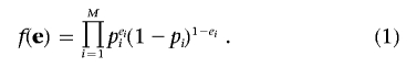
Let f(·) be the probability mass function of e. We first define a null model for the case in which there is only a single population. In this case, a natural null model is one that assumes that the components of e are independent, and each has probability of being 1, and 0 otherwise. Hence,

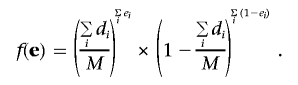Intuitively, if we do not have any information other than the disease status, the events that the individuals have the disease are independent, with the probability of disease obtained by plugging in the maximum-likelihood estimate. Note that the randomization test based on this null model is very close to the standard permutation test. The difference is that, in the permutation test, —that is, the number of the persons who have the disease stays the same for each resampling. In our case, this number is not fixed. Note, however, that since it is the sum of independent, identically distributed Bernoulli random variables, its distribution is concentrated around .

We now consider the case in which population stratification exists. In this case, it no longer suffices to consider a null model in which each person has the same probability of having the disease; rather, we need to obtain probabilities on the basis of estimates of the individual’s population.

Formally, let p denote the baseline probability vector, a vector whose components p_i denote the probability that the ith person has the disease, given the population structure. Since independence is assumed in this conditional distribution, we obtain the null model

The goal is to calculate the P value under this null model.

This procedure requires the baseline probability vector p as an input. This vector can be estimated by any of several methods. Since our focus in the present article is the subsequent step of computing statistical significance, we simply adapt an existing method to our purposes.

In particular, we have found that the following simple approach has worked well in practice. We used EIGENSTRAT,⁸ to find the eigenvectors that correspond to a small number of axes of variation (we used two axes in our experiments). We then projected individuals’ genotype data onto these axes and clustered the individuals by use of a K-means clustering algorithm (we used K=3 in our experiments). Finally, we obtained p_i for each person by computing a maximum-likelihood estimate based on the cluster assignments—that is, we set

where C_i is the set of indices for all individuals in the cluster to which the ith individual is assigned.

Given the baseline probability vector, we now wish to calculate the statistical significance of the association score. A naive approach to performing this calculation is to use a simple Monte Carlo sampling scheme. The algorithm samples e many times according to equation (1) and, for each sample, calculates the statistic S(G,e). The fraction of times that this statistic exceeds the original value S(G,d) is the estimated P value. We call this method the “standard sampling algorithm.” The running time of this approach is O(MNP_S), where P_S is the number of permutations.

Efficient Calculation

We now describe our approach that provides a computationally efficient alternative to the standard sampling algorithm. We use the methodology of importance sampling.¹⁶ Informally, in the standard sampling algorithm, samples are taken from the set of all possible disease vectors (2^M), which is a very large set. In PSAT, instead of sampling from this huge space, sampling is done from the space of all “important disease vectors”—namely, all possible disease vectors that give a larger association score than the original one.

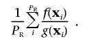
The importance sampling is done by repeated sampling of vectors from a sampling space 𝒢 with probability measure g that we define below. If P_R samplings are performed, and x_i is the ith sampled vector, then the P value is estimated by

The main steps of our algorithm are the same as in the simpler setting. (i) A column (or a SNP) is sampled. (ii) A contingency table is sampled for that column from the set of all possible contingency tables that are induced by this column and whose association score is at least as large as the original one. (iii) An important disease vector that is induced by this contingency table is sampled. The key underlying idea in this procedure is that, although the size of the set of all possible disease-vector instances may be very large, the number of all possible contingency tables is polynomial in the problem size.

Although our algorithm is similar in spirit to the importance sampler of Kimmel and Shamir,¹⁵ that method did not treat population stratification, and the analysis described there does not apply to our case. In particular, in our case, the different possible disease vectors are not equally probable, and this requires new algorithmic ideas, to which we now turn.

Let T be a contingency table, j be a column, and e be a sampling disease vector. For contingency table T, we use T_i,j to denote the component of the ith row of the jth column of T. We would like to calculate the conditional probability of an important sampling disease vector, given its inducing column. For that purpose, we use the factorization Pr(e|j)=Pr(e|T)Pr(T|j), which will be derived below. Intuitively, this equation holds because, given j, only one table T determines e. Our main effort, henceforth, is to show how to sample from and calculate both Pr(e|T) and Pr(T|j).

The sampling space 𝒢 is composed of the set of all possible disease vectors whose score equals or exceeds the original score. That is, 𝒢 contains the set of events {e|S(G,e)⩾S(G,d)}. We now define a probability measure on 𝒢 and show how to sample from it.

For a specific contingency table T, we write e≺T if the binary vector e is induced by T—that is, . In other words, the number of ones in e equals the number of diseased individuals according to T.

For a specific column j in G, let T_j be the set of all contingency tables with score equal to or larger than the original statistic. Hence, T_j:={T|∃e:T=Ω(G_i,j,e)∧A(T)⩾S(G,d)}. Each table in T_j induces many instances of the disease vector, and each of them may have a different probability.

To define a probability measure on 𝒢, we first define a probability measure on the columns. Let J_I be the set of all columns of G that induce at least one contingency table with a score larger or equal to that of the original statistic. We define

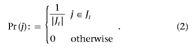We now investigate several properties of the events in 𝒢. The probability of a disease vector e, given contingency table T, is

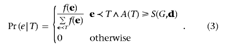Given a column j, the probability of table T is

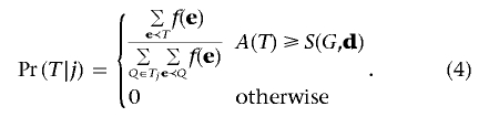Multiplying equation (3) by equation (4) gives

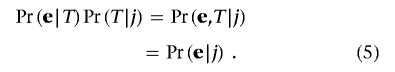The first equation follows from the fact that, once table T is given, the probability of e depends solely on T, so Pr(e|T)=Pr(e|T,j). The second equation holds because, given j, e is induced by exactly one table in T_j. The probability measure on 𝒢, denoted by g(·), is

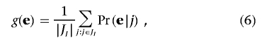where Pr(e|j) can be obtained by equation (5).

Next, we show how to calculate equations (3) and (4) efficiently. The challenge is to compute the sums in these equations. Calculating (here, Q is a contingency table) can be done directly by going over all possible tables in T_j in O(M²) time.

Calculating for a given contingency table, T, is more challenging. The number of all possible e induced by T is

which may be very large. This is solved by a dynamic programming approach. For table T, we build three different matrices—W₀, W₁, and W₂—one for each different type of marker: 0, 1, and 2, respectively. Since the construction of these three matrices is the same computationally, we will show how to generate W₀ only.

W₀ is of size M₀×(M₀+1), where M_i is the number of persons with locus type i. The components of W₀ are defined as follows. W₀(i,j) is the probability that the set of the first i individuals with locus type 0 contains exactly j individuals with the disease. Note that i goes from 1 to M₀, and j from 0 to M₀. We use the notation p⁽⁰⁾_i for the baseline probability of the ith person with locus type 0.

Initialization of W₀ is

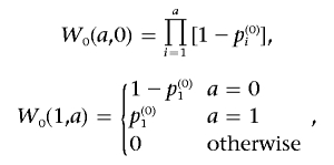and the transition is

Using these matrices, we have

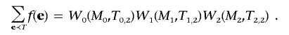To complete the description of the importance-sampling procedure, we need to show how we sample vector e from 𝒢. This is done in three steps. (i) Randomly choose a column j from the set J_I according to equation (2). (ii) Sample table T from T_j according to equation (4). (iii) Sample disease vector e from T according to equation (3).

Step (iii) in this algorithm cannot be performed directly because there are many possible disease vectors induced by T. The sampling can be done using the dynamic programming matrices W₀, W₁, and W₂. The idea is that, given the contingency table T, each set of components of e that correspond to persons with the same locus type can be drawn independently. Without loss of generality, we will show how to sample the set of components of e that correspond to persons with the locus type 0.

The sampling is done in W₀, starting at location W₀(M₀,T_0,2) and going backward. At location W₀(i,j), with probability

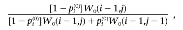go to W₀(i-1,j), and the corresponding ith individual with locus type 0 at e is set to 0. At location W₀(i,j), with probability

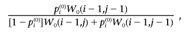go to W₀(i-1,j-1), and the corresponding ith individual with locus type 0 at e is set to 1. The process is stopped when i=j; in this case, all the persons with locus type 0 whose indices are smaller than i are set to 1.

The time complexity can be considerably reduced by exploiting the biological properties of the data set. We assume that two SNPs that are separated by C or more SNPs along the genome are independent, because of the LD decay along the chromosome. C is called the “linkage upper bound” of the data.

According to equation (6), the probability of the sampled disease vector e is the average of Pr(e|T_j). Observe that, if A(e,d)<S(G,d), then Pr(e|T_j)=0. Using the LD decay property, we expect that e and SNPs that are far apart will be independent. Hence, when g(e) is calculated for each vector e, it is unnecessary to range over all N SNPs; only SNPs within a distance of C need to be checked. The rest of the SNPs are independent of the chosen column, so the expected number of columns that give a score higher than S(G,d) is (N-2C-1)q, where q is the probability that a single column will result in a higher score than S(G,d). Note that q need be calculated only once at the preprocessing step. Consequently, only O(MC) operations are needed to calculate g(e), instead of O(MN) operations. For each permutation, a total of O(M²) operations are required to go over all contingency tables and to build the dynamic programming tables. In summary, the total running time of the algorithm is O[P_R(M²+MC)].

Results

Data Sets

We used the HapMap resource, using SNPs from the Affymetrix GeneChip Human Mapping 500K Array Set. We used only SNPs that were typed in all three populations: YRI (Yoruba people of Ibadan, Nigeria), ASI (Asian population), and CEU (population of western European ancestry). We excluded the X chromosome. Overall, 477,714 SNPs were used.

Comparison with Previous Methods

We compared PSAT with genomic control⁹ and EIGENSTRAT.⁸ It was not possible to apply structured association^12,13 and the mixed-model method¹¹ to our data sets, because of the high computational cost incurred by these methods. Comparison with the recent work of Epstein et al.¹⁷ was also not possible, because the software is available only as an implementation that uses commercial software. However, it is noteworthy that, similar to previous methods, the mixed-model and the methods of Epstein et al.¹⁷ do not account for the LD structure.

For each method, a study was defined to be significant if the P value, calculated as the statistic of the most associated SNP, was <.05. False-positive rate and power were calculated by performing 100 different experiments. PSAT calculates the P value directly, and, for genomic control and EIGENSTRAT, we used a Bonferroni correction. There may be better ways to correct for multiple testing with these methods, but, as was mentioned above, it is not clear which approach would be better. Simply permuting the cases and controls would be wrong statistically, since this assumes that the chance of having the disease is equal among all individuals from all populations. Note that, when false-positive rates are measured, this conservative correction gives an advantage over EIGENSTRAT and genomic control.

False-positive rates

The simulations conducted by Price et al.⁸ used the Balding-Nichols model to generate different populations. Although this approach matches F_ST between simulated populations and real ones, two key aspects of that simulation are unrealistic. First, according to this model, SNPs are sampled independently. (F_ST compares the genetic variability within and between different populations.¹⁸) In real whole-genome studies, there is a strong correlation between nearby SNPs. Second, according to the model of Price et al.,⁸ for each SNP, an ancestral-population allele frequency p was drawn from the uniform distribution on [0.1,0.9]. The allele frequencies for populations 1 and 2 were each drawn from a beta distribution with parameters p(1-F_ST)/F_ST and (1-p)(1-F_ST)/F_ST. For F_ST=0.004, the value used in that study, this gives practically zero probability (<10⁻¹⁶) that a SNP has frequency 0 or 1, whereas, in real populations, there are many examples of SNPs that present only one allele in one population while, in the other population, both alleles are observed. To provide a more realistic test of PSAT, we worked with real SNPs from the HapMap project.

To generate additional haplotypes based on haplotypes identified by the HapMap project, we used the stochastic model of Li and Stephens¹⁹ as a generative procedure. This is done as follows.¹⁵ Suppose k haplotypes are currently available. Then, the (k+1)st haplotype is generated in two steps. First, recombination sites are determined assuming a constant recombination rate along the chromosome. Second, for each stretch between two neighboring recombination sites, one of the k haplotypes is chosen with probability 1/k. The process is repeated until the required number of haplotypes is obtained. The recombination rate along this process is 4N₀r/k, where r is the probability of recombination between two adjacent sites per meiosis, set to 10^-8, and N₀ is the effective population size, set to 10,000. This approach preserves the dependency between nearby SNPs, and the resulting data sets mimic real scenarios more accurately.

The first set of experiments was done on mixtures of more than one population, under the assumption that there is no causal SNP. This was done by randomly assigning different population types to the cases and the controls. In all tests, we had 500 cases and 500 controls, and we used the 38,864 SNPs on chromosome 1. Population acronyms are adopted from the HapMap project (see the “Methods” section), and we use “ASI” for the Asian population (including Japanese from Tokyo and Han Chinese from Beijing).

The following tests were done. (i) All the controls were sampled from population CEU, and the cases were sampled as an (r,1-r) mixture of populations CEU and ASI, respectively. (ii) Cases were sampled as an [r,(1-r)/2,(1-r)/2] mixture of populations CEU, ASI, and YRI, respectively. Controls were sampled as an [r,(1-r)/2,(1-r)/2] mixture of populations YRI, ASI, and CEU, respectively. For both (i) and (ii), we tried different values of r: r=0.1, 0.2,…, 0.9. The results are presented in figure 1.

Figure 1. .

Comparison of false-positive rate between PSAT, EIGENSTRAT, and genomic control. The data set was composed of 500 cases and 500 controls sampled from three populations: CEU, ASI, and YRI. A, Cases sampled as an (r,1-r) mixture of populations CEU and ASI, respectively, and controls sampled from CEU. B, Cases sampled as an [r,(1-r)/2,(1-r)/2] mixture of populations CEU, ASI, and YRI, respectively, and controls sampled as an [r,(1-r)/2,(1-r)/2] mixture of YRI, ASI, and CEU, respectively. Note that, in panel A when r=1 and in panel B when r=1/3, the cases and the controls have the same population structure. All methods perform well when r is close to this value. Each dot represents the average of 100 experiments.

Given that there is no causal SNP in this test, the false-positive rate is the fraction of the experiments with P<.05. In all the experiments, PSAT’s false-positive rate was <0.05 and was lower than or equal to that of the other two methods. Generally, EIGENSTRAT was more accurate than genomic control when applied to a mixture of two populations and was less accurate for a mixture of three populations. Both of the methods exhibited a false-positive rate of 1.0 in several cases (fig. 1).

Power

To study the power of the methods, we applied them to a case-control study, where the cases were sampled as an (r,1-r) mixture of populations CEU and ASI, respectively, and controls were sampled from CEU. We used a multiplicative model for generating samples of cases and controls. We simulated panels with 1,000 cases and 1,000 controls, and the first 10,000 SNPs of chromosome 1. For each panel, a SNP was randomly chosen to be the causal SNP and was then removed from the panel. We set the disease prevalence to 0.01 and the relative risk to 1.5.

To compare the power of the different methods, one needs to fix the false-positive rate. Doing this is not straightforward because, as described above, when population stratification exists, EIGENSTRAT and genomic control have high false-positive rates (and thus also have high but meaningless ”power”), whereas PSAT maintains a false-positive rate <0.05. To overcome this problem, we artificially adjusted the power of EIGENSTRAT and genomic control as follows. For each value of r, we generated 100 additional panels with the same population structure, without a causal SNP. We then applied both algorithms to these data sets. The 5% quantile of the obtained P values was used as the new threshold for statistical significance, instead of .05. (When population structure exists, this threshold is <.05.) To estimate power, an additional 100 panels with causal SNPs were simulated. By use of this approach, the power is evaluated while the significance (type I error rate) is fixed to 0.05.

The results are presented in figure 2. For the P value threshold of .05, the advantage in the power of PSAT over EIGENSTRAT reaches up to 14%. A more prominent difference is observed between PSAT and genomic control. A power comparison for a single population (CEU) when there is a causal SNP is presented in figure 3, for different P value cutoffs. Since no stratification exists in this case, there is no need to control the P value artificially. Again, PSAT shows a consistent advantage. In this experiment, the naive Bonferroni correction also obtained higher power than EIGENSTRAT.

Figure 2. .

Power comparison between PSAT, EIGENSTRAT, and genomic control. The data sets were composed of 1,000 cases and 1,000 controls. Cases were sampled as an (r,1-r) mixture of populations CEU and ASI, and controls were sampled from CEU. The power is adjusted for all methods for a statistical significance level of .05.

Figure 3. .

Power comparison for one population (i.e., when there is no population structure in the data) between PSAT, Bonferroni correction, EIGENSTRAT, and genomic control. The data sets were composed of 1,000 cases and 1,000 controls from the CEU population.

Finding several causal SNPs

We tested the performance of the algorithms for discovering several hidden causal SNPs. For that, we repeated the above experiments, with all the controls sampled from population CEU and the cases sampled as an (r,1-r) mixture from populations CEU and ASI, respectively. Of the 10,000 SNPs, we randomly chose 2 causal SNPs, each with risk ratio of 1.5. In each algorithm, we used the ranking of the ordered P values obtained separately for each SNP. A discovery was defined if a SNP at a distance of <10 kb from a causal SNP appeared in the top 100 ranked SNPs. To calculate the discovery rate, each of the experiments was repeated 100 times. The comparison is summarized in figure 4. As can be observed, PSAT shows a higher discovery rate than that of the other algorithms. As expected, the advantage is more prominent when the level of population stratification is higher. Since genomic control does not reorder the scores, the results presented for it and for the original scores are the same.

Figure 4. .

Comparison of causal SNP discovery rate when there are two causal SNPs. The data sets were composed of 1,000 cases and 1,000 controls from a mixture of CEU and ASI populations, as in figure 2. Each panel contains two hidden causal SNPs. For each algorithm, a discovery of a causal SNP was defined as the event where a SNP within 10 kb of a causal SNP was among the 100 top-ranked SNPs.

Running Time

To illustrate the essential role played by the importance-sampling procedure in our approach, we conducted a large-scale experiment, using all SNPs from the Affymetrix 500K GeneChip for all chromosomes (477,714 SNPs in total). We used 1,000 cases and 1,000 controls. In this setting, the running time for each step of a naive sampling algorithm was 66 s on a powerful workstation (Sun Microsystems Sun Fire V40z workstation with a Quad 2.4 GHz AMD Opteron 850 Processor and 32 GB of RAM). Hence, to obtain an accuracy of 10^-6 (which requires ∼10⁶ samples), ∼764 d are required, and, for a P value of 10^-4, ∼8 d are required. The PSAT algorithm finishes in 22 min in both cases.

Evaluating Accuracy and Convergence of the Importance-Sampling Algorithm

Since PSAT is based on importance sampling, it is important to test the variance of the obtained P values and to check convergence to the correct P value. We sampled cases and controls from one population (CEU), as described in the “Methods” section. We estimated the SD for each single run of the algorithm, on the basis of the variance of the importance-sampling weights. The relation between the SD and the P value is presented in figure 5. It can be observed that the SD is ∼1/10 of the P value.

Figure 5. .

SD and P value. The X-axis is the logarithm of the P value. The Y-axis is the logarithm of the SD of the P value. Data sets comprised 100 cases and 100 controls sampled from the CEU population. Logarithms are base 10.

To verify convergence of the importance sampling to the standard sampling algorithm empirically, we conducted 100 experiments with 100 cases and 100 controls, using 1,000 SNPs. (We used a limited number of SNPs and individuals in this experiment, to be able to perform many samplings of the standard sampling algorithm.) We applied PSAT with importance sampling and the standard sampling version of PSAT with 10⁶ permutations. CIs were calculated on the basis of the estimated SD of the standard sampling test. Convergence was defined to be correct if the P value obtained by the importance sampling technique was in the CI of the standard sampling algorithm. PSAT converged to the correct result in all 100 experiments.

Discussion

We have presented a methodology for controlling for population structure on the basis of randomization tests. The method is a conditional method that takes into account both population structure and dependencies between markers. This yields an increase in power relative to that of competing methods.

Our simulations also show that existing methods can consistently fail to correct for stratification on mixtures of several populations, yielding high false-positive rates. When different levels of population mixture are considered, both genomic control and EIGENSTRAT have relatively high false-positive rates, whereas PSAT maintains a constant false-positive rate, which equals the threshold P value (.05), as required. This can be explained by the fact that PSAT accounts more accurately for the population stratification effect.

In practice, one would aim to obtain an even mixture of cases and controls; however, one would like to use a method that is robust to uncontrolled mixing. Indeed, although it is desirable and, in some cases, attainable, many association studies contain a mixture of several distinct populations. For instance, Stranger et al.²⁰ recently identified and characterized functionally variable genomic regions contributing to gene-expression differences through effects on regulation of gene expression. To achieve this goal, they produced a large data set of mRNA transcript levels obtained from 270 individuals from four populations of the HapMap project. Another example is the study by Aranzana et al.,²¹ in which genomewide polymorphism data and phenotypes were collected for different types of Arabidopsis. Another interesting example is a study conducted on a mixture of diverse populations by Sutter et al.²² They used the breed structure of dogs to investigate the genetic basis of size and found that a single IGF1 SNP is common to all small breeds and is nearly absent from giant breeds, suggesting that the same causal sequence variant is a major contributor to body size in all small dogs. In all these examples, the complex population structure and the wide diversity were exploited to obtain a more accurate association mapping.

The power of PSAT is higher than that of the other methods, because the LD structure is exploited by PSAT. For example, when the mixture is even, the false-positive rate of EIGENSTRAT approaches that of PSAT, but the power of PSAT is larger by 10%. When different population mixtures were tested, we adjusted the thresholds of the other methods so that the significance is set to .05 (equal to that of PSAT). In this case, we observed that the power of PSAT is higher than that of the other methods by up to 14%. It is important to note that such adjustment might be impossible to apply in real scenarios, since it depends on the existence of panels with exactly the same population structure and without a causal SNP. In such situations, one cannot predict the false-positive rate of these methods, because it depends on the population structure. Put differently, the P value obtained by them will be uncalibrated.

It is interesting to note that, although EIGENSTRAT performed well in the sense of inferring population structure—thus supporting our tentative choice of EIGENSTRAT as a procedure for estimating the baseline probability vector—the subsequent correction computed by EIGENSTRAT was not always accurate. Indeed, in extreme cases, we saw that EIGENSTRAT yielded a false-positive rate of 1. It is important to emphasize the general point that computing an accurate correction is not a straightforward consequence of obtaining an accurate estimate of population structure. In the specific case of EIGENSTRAT, we provide an explanation of this decoupling of correction estimation and population structure estimation in appendix A. The high false-positive rate obtained by genomic control can be explained by its artificial assumption that the null is a multiplication of the χ² distribution. This issue was already raised by Marchini et al.²³ We observed experimentally that the null of a mixture of populations is not distributed as an inflated χ² distribution (data not shown).

In general, the computational feasibility of PSAT depends on its exploitation of dynamic programming and importance sampling. It is worth noting, however, that the advantage of importance sampling is significant only when the P value is small (⩽10^-4); if only large P values (say, .05) are of interest, then it is possible to dispense with importance sampling. We do not regard the use of large P values as a satisfactory strategy, however. Small P values are desirable in the context of making decisions about whether to follow up on an association result and are likely to become increasingly important in forthcoming large-scale association studies. See the work of Kimmel and Shamir¹⁵ and Ioannidis et al.²⁴ for further discussion of this issue. Running time is also important for simulation purposes—for example, when it is required to calculate P values across simulated panels to estimate the power of a method. In this setting, a fast algorithm for calculating the significance is essential.

It is possible to handle missing data within the PSAT framework simply by adding another row to the contingency table containing the number of individuals with missing data. Note that the time complexity of ranging over contingency tables is still polynomial in this case; moreover, the running time remains independent of the number of SNPs. Other covariates, such as age and sex, can be used by incorporating them into the baseline probability vector. Continuous traits, such as blood pressure, can be treated by the standard sampling of PSAT. It is less straightforward, however, to adopt the importance sampling algorithm to continuous traits, because the reduction to contingency tables is not possible in this case.

Although we have focused on controlling the error probabilities associated with the maximum of the SNP scores, other statistics can also be used within the PSAT framework. One interesting example is the minimum of the top k scores of the SNPs. This would be more appropriate if one wants to choose the k best SNPs to conduct further investigation in the next research phase.

In many cases, ordering of the SNPs according to their association score is used to select the most-promising SNPs for a follow-up study or investigation. We explored this by calculating the P value for each SNP separately with PSAT and used it as the ranking score. Similar to EIGENSTRAT and as opposed to genomic control, PSAT reorders the ranking of the scores. This can be of great importance, since two different SNPs might be assigned the same score by the standard association function, whereas one is more biased by the population structure than the other. Our experiments show that this issue has important implications for locating the correct causal SNPs. The advantage of PSAT over EIGENSTRAT, in terms of discovery rate, is up to 12%. The even higher difference from genomic control (>55%) can be explained by the unordered approach taken by genomic control.

Our approach has some family resemblance to the recent work of Epstein et al.¹⁷ In particular, both approaches use a two-step procedure—first finding a vector that represents population structure (the baseline probability vector in PSAT and the estimated odds of disease in the approach of Epstein et al.¹⁷) and then using this vector to correct for stratification. The second step, however, is rather different in the two cases. Epstein et al. use stratified logistic regression, with the subjects clustered into one of five strata based on quartiles of the stratification scores. In contrast, our method uses the baseline probability vector as the null model itself and does not assume a constant number of clusters. Most importantly, PSAT takes the complex LD structure into account by sampling from this null model.

We emphasize that the focus of our work is a method for correcting for stratification given the baseline probability vector. We have deliberately avoided the complex question of how to infer the population structure, since our focus is the correction. In our work to date, we have used EIGENSTRAT for this purpose. It is noteworthy that, in some cases, inferring the baseline probability vector can be more challenging, and this simple approach would fail. For example, in an admixed population, none of the individuals can be classified globally into one of a limited number of clusters. Another example is an individual that does not fall into any of the clusters. As we have noted, however, other methods, including STRUCTURE,¹² can be used to provide these estimates, and, in some cases, they should be tailored specifically to the studied data, according to the known population history. Our approach makes no specific assumption regarding the model used to provide estimates; any method that estimates probabilities that each individual has a disease on the basis of (solely) the population structure can be employed within our approach.

In particular, we do not require modeling assumptions, such as a constant number of ancestry populations. The baseline probability vector can contain distinct probabilities for all its components. This property is of importance for several scenarios. One example is presented by Pritchard et al.¹²: species live on a continuous plane, with low dispersal rates, so that allele frequencies vary continuously across the plane. In PSAT, one can calculate the components of the baseline probability vector for each individual on the basis of the near neighbors. This avoids the assumption of a constant number of populations. Thus, the PSAT framework is naturally upgradeable as new methods for inferring population structure become available. Finally, although we have observed empirically that the population estimates provided by EIGENSTRAT seem to be adequate for subsequent computations of corrections by PSAT, it would be useful to attempt an analysis of the statistical robustness of PSAT to errors in the population structure estimates.

Appendix A

In this appendix, we provide an explanation for the failure of EIGENSTRAT to correct stratification. We show that, even if the population structure is inferred accurately, use of the structure as a covariate in a multilinear regression may lead to spurious results. To illustrate this issue, consider the extreme situation in which the sample contains cases from one population and controls from another population. The correction of EIGENSTRAT is as follows. For each SNP vector, subtract its projections onto the axes of variation. Do the same for the disease vector. Then, check whether a trend exists between the corrected SNP and disease vectors (by an Armitage trend test).

For simplicity, assume that we have only a single axis of variation (as is usually done in the case of two populations). Consider the graphical illustration in figure A1. In two different populations, there are usually few SNPs with the property that one allele frequency is close to 1 in one population and close to 0 in the other (i.e., in the other population, most of the individuals have the other allele). This SNP and the disease vector point in the same direction. If the axis of variation is the true one, then it also points in the same direction. Decreasing the projections of these two vectors onto the axis of variation gives two zero vectors, and the trend is not significant, as required. The problem is that, in real data sets, the axis of variation is not exactly in the true direction but might be very close to it. Since the SNP and the disease vectors are in the same direction, the resulting subtracted vectors are in the same direction, which gives a very high trend score, yielding a false-positive result.

Figure A1. .

Illustration of the correction made by EIGENSTRAT. , , and are vectors that represent the SNP, disease, and axis of variation vectors, respectively. Observe that the projections of and on are and , respectively, since is a unit length, so that . The two dashed vectors are the vectors obtained after the correction, and the trend test is performed on them. If is in exactly the same direction as and , then the adjusted vectors become zero, and there is no trend. However, any small change in will give two strongly correlated adjusted vectors, with a significant trend test.

Most importantly, there is no correlation between the amount of change in the axis of variation and the correction error. Any slight change in this axis can lead to false-positive results. To see this, consider an inaccuracy angle of ɛ between , the population vector, and , the SNP vector (fig. A1). The trend score calculated between the adjusted vectors—that is, and —is M (the number of samples), since these vectors are parallel, so that the correlation coefficient is 1 and the trend-test statistic is defined to be M times the square of the correlation. Hence, the high score obtained in this case, M, is independent of the amount of inaccuracy, ɛ. Therefore, the method is very sensitive to small changes in the axis of variation. Such small changes in this axis might occur as a result of sampling error.

Note that it is not obligatory that all cases and controls are from different populations for the correction of EIGENSTRAT to be wrong. It suffices to have a single SNP with the property described above, so long as the axis of variation is not exactly in the correct direction. These two conditions seem likely to hold in many data sets; therefore, we anticipate that the EIGENSTRAT correction will often be inaccurate. As expected and as can be observed from our experiments, the closer the structure of the cases and the controls, the less inaccurate the correction.

References

- 1.Freedman ML, Reich D, Penney KL, McDonald GJ, Mignault AA, Patterson N, Gabriel SB, Topol EJ, Smoller JW, Pato CN, et al (2004) Assessing the impact of population stratification on genetic association studies. Nat Genet 36:388–393 10.1038/ng1333 [DOI] [PubMed] [Google Scholar]
- 2.Clayton DG, Walker NM, Smyth DJ, Pask R, Cooper JD, Maier LM, Smink LJ, Lam AC, Ovington NR, Stevens HE, et al (2005) Population structure, differential bias and genomic control in a large-scale, case-control association study. Nat Genet 37:1243–1246 10.1038/ng1653 [DOI] [PubMed] [Google Scholar]
- 3.Lander ES, Schork NJ (1994) Genetic dissection of complex traits. Science 265:2037–2048 10.1126/science.8091226 [DOI] [PubMed] [Google Scholar]
- 4.Helgason A, Yngvadottir B, Hrafnkelsson B, Gulcher J, Stefansson K (2005) An Icelandic example of the impact of population structure on association studies. Nat Genet 37:90–95 [DOI] [PubMed] [Google Scholar]
- 5.Campbell CD, Ogburn EL, Lunetta KL, Lyon HN, Freedman ML, Groop LC, Altshuler D, Ardlie KG, Hirschhorn JN (2005) Demonstrating stratification in a European American population. Nat Genet 37:868–872 10.1038/ng1607 [DOI] [PubMed] [Google Scholar]
- 6.Hirschhorn JN, Daly MJ (2005) Genome-wide association studies for common diseases and complex traits. Nat Rev Genet 6:95–108 10.1038/nrg1521 [DOI] [PubMed] [Google Scholar]
- 7.Lohmueller K, Lohmueller KE, Pearce CL, Pike M, Lander ES, Hirschhorn JN (2003) Meta-analysis of genetic association studies supports a contribution of common variants to susceptibility to common disease. Nat Genet 33:177–182 10.1038/ng1071 [DOI] [PubMed] [Google Scholar]
- 8.Price AL, Patterson NJ, Plenge RM, Weinblatt ME, Shadick NA, Reich D (2006) Principal components analysis corrects for stratification in genome-wide association studies. Nat Genet 38:904–909 10.1038/ng1847 [DOI] [PubMed] [Google Scholar]
- 9.Devlin B, Roeder K (1999) Genomic control for association studies. Biometrics 55:997–1004 10.1111/j.0006-341X.1999.00997.x [DOI] [PubMed] [Google Scholar]
- 10.Devlin B, Bacanu S, Roeder K (2004) Genomic control to the extreme. Nat Genet 36:1129–1130 10.1038/ng1104-1129 [DOI] [PubMed] [Google Scholar]
- 11.Yu J, Pressoir G, Briggs WH, Bi IV, Yamasaki M, Doebley JF, McMullen MD, Gaut BS, Nielsen DM, Holland JB, et al (2006) A unified mixed-model method for association mapping that accounts for multiple levels of relatedness. Nat Genet 38:203–208 10.1038/ng1702 [DOI] [PubMed] [Google Scholar]
- 12.Pritchard JK, Stephens M, Donnelly P (2000) Inference of population structure using multilocus genotype data. Genetics 155:945–959 [DOI] [PMC free article] [PubMed] [Google Scholar]
- 13.Pritchard JK, Stephens M, Rosenberg NA, Donnelly P (2000) Association mapping in structured populations. Am J Hum Genet 67:170–181 [DOI] [PMC free article] [PubMed] [Google Scholar]
- 14.Rosenberg NA, Nordborg M (2006) A general population-genetic model for the production by population structure of spurious genotype-phenotype associations in discrete, admixed, or spatially distributed populations. Genetics 173:1665–1678 10.1534/genetics.105.055335 [DOI] [PMC free article] [PubMed] [Google Scholar]
- 15.Kimmel G, Shamir R (2006) A fast method for computing high significance disease association in large population-based studies. Am J Hum Genet 79:481–492 [DOI] [PMC free article] [PubMed] [Google Scholar]
- 16.Kalos MH (1986) Monte Carlo methods. John Wiley and Sons, New York [Google Scholar]
- 17.Epstein MP, Allen AS, Satten GA (2007) A simple and improved correction for population stratification in case-control studies. Am J Hum Genet 80:921–930 [DOI] [PMC free article] [PubMed] [Google Scholar]
- 18.Hudson RR, Slatkin M, Maddison WP (1992) Estimation of levels of gene flow from DNA sequence data. Genetics 132:583–589 [DOI] [PMC free article] [PubMed] [Google Scholar]
- 19.Li N, Stephens M (2003) Modelling linkage disequilibrium and identifying recombinations hotspots using SNP data. Genetics 165:2213–2233 [DOI] [PMC free article] [PubMed] [Google Scholar]
- 20.Stranger BE, Nica A, Bird CP, Dimas A, Beazley C, Dunning M, Thorne N, Forrest MS, Ingle CE, Tavare S, et al (2007) Population genomics of human gene expression. Presented at the Biology of Genomes Meeting, Cold Spring Harbor Laboratory, Cold Spring Harbor, NY, May 8–12 [Google Scholar]
- 21.Aranzana MJ, Kim S, Zhao K, Bakker E, Horton M, Jakob K, Lister C, Molitor J, Shindo C, Tang C, et al (2005) Genome-wide association mapping in Arabidopsis identifies previously known flowering time and pathogen resistance genes. PLoS Genet 1:531–539 10.1371/journal.pgen.0010060 [DOI] [PMC free article] [PubMed] [Google Scholar]
- 22.Sutter NB, Bustamante CD, Chase K, Gray MM, Zhao K, Zhu L, Padhukasahasram B, Karlins E, Davis S, Jones PG, et al (2007) A single IGF1 allele is a major determinant of small size in dogs. Science 316:112–115 10.1126/science.1137045 [DOI] [PMC free article] [PubMed] [Google Scholar]
- 23.Marchini J, Cardon LR, Phillips MS, Donnelly P (2004) Genomic control to the extreme. Nat Genet 36:1129–1131 10.1038/ng1104-1129 [DOI] [PubMed] [Google Scholar]
- 24.Ioannidis JPA, Trikalinos TA, Ntzani EE, Contopoulos-Ioannidis DG (2003) Genetic association in large versus small studies: an empirical assessment. Lancet 361:567–571 10.1016/S0140-6736(03)12516-0 [DOI] [PubMed] [Google Scholar]