Possible Biomechanical Origins of the Long-Range Correlations in Stride Intervals of Walking

Abstract

When humans walk, the time duration of each stride varies from one stride to the next. These temporal fluctuations exhibit long-range correlations. It has been suggested that these correlations stem from higher nervous system centers in the brain that control gait cycle timing. Existing proposed models of this phenomenon have focused on neurophysiological mechanisms that might give rise to these long-range correlations, and generally ignored potential alternative mechanical explanations. We hypothesized that a simple mechanical system could also generate similar long-range correlations in stride times. We modified a very simple passive dynamic model of bipedal walking to incorporate forward propulsion through an impulsive force applied to the trailing leg at each push-off. Push-off forces were varied from step to step by incorporating both “sensory” and “motor” noise terms that were regulated by a simple proportional feedback controller. We generated 400 simulations of walking, with different combinations of sensory noise, motor noise, and feedback gain. The stride time data from each simulation were analyzed using detrended fluctuation analysis to compute a scaling exponent, a. This exponent quantified how each stride interval was correlated with previous and subsequent stride intervals over different time scales. For different variations of the noise terms and feedback gain, we obtained short-range correlations (α < 0.5), uncorrelated time series (α = 0.5), long-range correlations (0.5 < α < 1.0), or Brownian motion (α > 1.0). Our results indicate that a simple biomechanical model of walking can generate long-range correlations and thus perhaps these correlations are not a complex result of higher level neuronal control, as has been previously suggested.

1. INTRODUCTION

The basic unit of measure in human walking is the stride, which defines one complete gait cycle. When humans walk, the time it takes to execute each stride varies from one stride to the next. In healthy adults walking at comfortable speeds over level ground, the time series of stride times exhibits long-range correlations (i.e., 1/f noise) where each stride is correlated with tens to hundreds of prior strides, and these correlations decay in a scale-free fractal-like manner [1, 2]. It has been proposed that these long-range correlations characterize a healthy system [3]. When the system deteriorates due to age or disease, time series fluctuations become more uncorrelated, or random. These changes occur in elderly subjects [4], patients with Huntington’s disease [4], and Parkinson’s patients [5]. Stride interval correlations also change in response to external stressors. When humans walk at a forced slower or faster gait speed, the long-range correlations in their stride times increase slightly [2]. When subjects’ stride times are externally constrained by having them follow the timing of a fixed external cadence (i.e., a metronome), their stride times become uncorrelated [2]. Thus, the long-range correlations in gait cycle timing can be modified by voluntary central nervous system (CNS) intervention and also deteriorate when the CNS is diseased. Based on these findings, it has been postulated that long-range correlations are regulated by central control mechanisms in the brain. This theory was further supported by recent findings that long-range correlations remained intact in patients with significant peripheral nerve degeneration [6].

To understand the origin of these correlations, several models have been proposed [1, 7–9]. These models are primarily based on the idea that human walking is regulated via oscillatory networks of neurons in the spinal cord known as central pattern generators (CPGs) [2, 8]. These models typically assume that the CPG acts as a nonlinear oscillator [8] which produces self-sustaining patterns of walking. Hausdorff et al. [1] proposed a stochastic CPG model to produce stride time fluctuations. Allowing the CPG frequency to vary randomly did not yield long-range correlations in the simulated stride times. However, when they introduced “memory” into their CPG by allowing transitions from frequency to frequency in a specific predefined way, then they did obtain long-range correlations [1]. Ashkenazy et al. [7] extended this approach by defining a neural ‘hopping’ model, where movement from one neural center to another was accomplished by a random walk. They assumed that as individuals matured, their neural interconnectedness would increase. By modeling the increase in interconnectedness as an increase in the range of hopping sizes, they were able to reproduce the changes in gait dynamics observed from childhood to adulthood [7]. West et al. [8] proposed a “super CPG” (SCPG) model that was similar to that of Ashkenazy except the stochastic correlated CPG was coupled to a forced van der Pol oscillator. They assumed that the strength of the correlations among the neural centers increased as the system was stressed (as in changing gait speed) and the intensity of the force driving the system increased with the conscious effort to walk at a controlled pace. This model reproduced the changes in long-range correlations seen in walking at faster and slower paces, and walking to a metronome [8].

While these models do reproduce the changes in stride time fluctuation dynamics observed experimentally, they do not necessarily exclude alternative, possibly simpler, explanations. In many cases where people have proposed that long-range correlations reflect complex self-regulating processes, others have provided much simpler explanations (e.g., [10, 11]). In particular, this has occurred in the closely related context of analyzing the fluctuations of the center of pressure (COP) trajectories exhibited by humans during quiet standing. Collins and DeLuca [12, 13] introduced a stabilogram diffusion analysis method to analyze center of pressure trajectories by methods similar to those used for analyzing stride times. They showed that COP trajectories in humans exhibit persistent (long-range) correlations over short time scales and anti-persistent (short-range) correlations over longer time scales. These fractal-like structures changed with variations in visual input [14], touch and vision [15], age [16], and disease [17]. Collins and his colleagues thus proposed a “pinned polymer model” of postural control to explain these seemingly complex correlation structures [18–20]. However, Peterka [21] replicated the majority of these seemingly complex behaviors by modeling the body as a single-link inverted pendulum controlled by a standard proportional, integral, and derivative (PID) controller driven by noisy sensory signals with physiological time delays. If a simple mechanical model with noisy feedback and physiological time delays can replicate the apparently complex dynamics observed during human standing, then perhaps the long-range correlations observed during human walking may similarly be explainable by relatively simple mechanical and neurophysiological (e.g., spinal reflex) mechanisms. Support for this idea can be found in Hausdorff and Peng’s model of ‘multi-scaled randomness’ [22]. The model output was simply the sum of random inputs occurring on different time scales. For certain combinations of parameters, they were able to obtain 1/f noise.

Only one primarily mechanical model has been studied for its ability to generate long-range correlations. Hausdorff et al. [1] modeled the lower leg as a free-swinging pendulum with mass attached with damping and spring elements to represent the muscles, tendons, and ligaments of the leg. The system was driven using a simple coupled oscillator with and without additive noise [1]. This model failed to produce any long-range correlations. However, this model only included a single leg and an unrealistic interaction with the ground and thus was not a model of “walking.” The purpose of the present study was therefore to determine if a simple mechanical model of walking incorporating noise and minimal feedback control could generate long-range correlations similar to those observed in humans. If true, this would suggest that the long-range correlations in human stride intervals might be explained by far simpler mechanisms than those proposed to date.

2. MODEL

We modified a simplified 2D model of passive dynamic walking [23]. The model (Figure 1) consisted of two legs connected by a frictionless hip joint and point masses at the feet and hip. The model assumed perfectly plastic collisions with the ground at foot strike and exhibited orbitally stable limit cycle dynamics when walking down shallow slopes, (γ) up to about 0.019 rad [23]. A push-off impulse (P_i) was added to generate the energy needed to replace the energy lost at each foot-strike collision. The model ignored “foot scuffing” interactions with the ground during the forward leg swing, as these could be easily avoided with an infinitesimal lifting of the foot [23, 24]. Assuming the foot masses were negligible compared to the hip mass, the model was governed by two second order equations of motion that describe the angular motion of the two legs about the foot and hip [23] (Eqs. 1). In equations 1a and 1b, time was rescaled by a factor $\sqrt{l/g}$.

Figure 1.

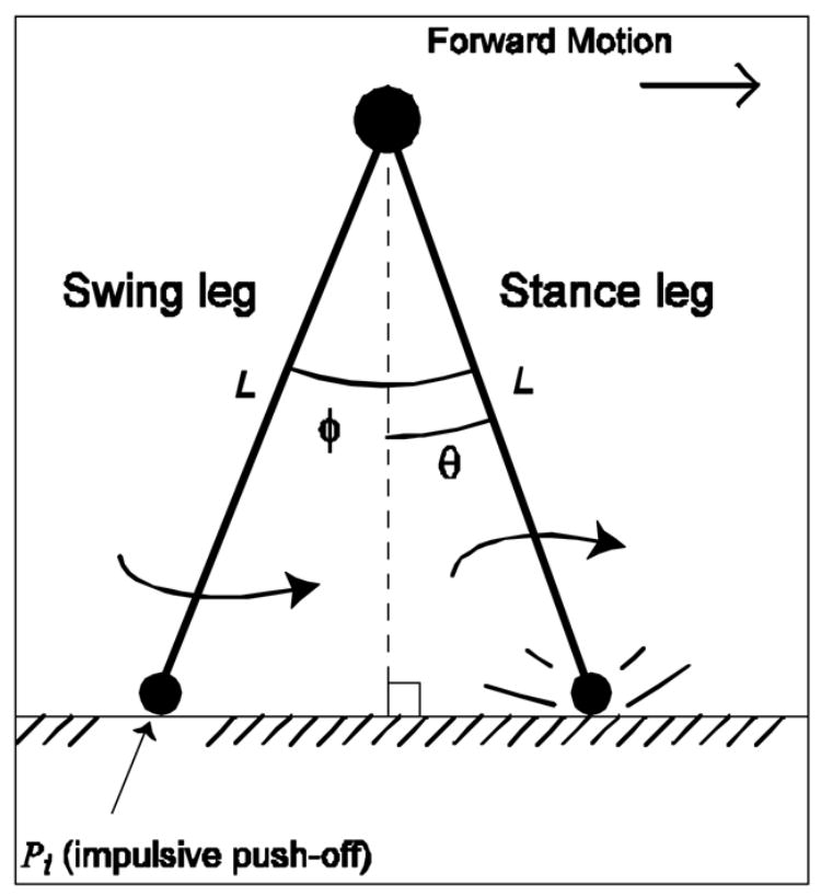
The model was adapted from the “simplest walking model” [22, 25]. The model had four state variables defined by the model’s 2 degrees of freedom, θ and φ, and their corresponding angular velocities. θ was the angle between the front leg and a line perpendicular to the walking surface and φ was the angle between the two legs. Foot strike was defined as the instant in time when φ – 2θ = 0. At this point, the state variables were put through the transition matrix that switched the stance and swing legs. Additionally, a variable impulsive force (Eq. 4) was applied to the swing leg to give it enough energy to redirect the center of mass upward and forward. This allowed the model to walk over level ground [25].

$$\ddot{\theta }(t)-sin(\theta (t)-\gamma )=0$$ (1a)

$$\ddot{\theta }(t)-\ddot{\phi }(t)+\dot{\theta }{(t)}^{2}sin\phi (t)-cos(\theta (t)-\gamma )sin\phi (t)=0$$ (1b)

Walking data were generated by integrating equations (1a) and (1b) through one complete step of the swing leg with γ = 0. All integrations were performed in Matlab using the fourth-order Runga Kutta method (ode45) with the error tolerance set to 10⁻¹². The swing foot contacted the ground (i.e., foot strike occurs) when the two feet were symmetrically oriented about the normal to the flat walking surface:

$$\phi -2\theta =0$$ (2)

At this point, a foot strike transition rule (Eq. 3) was applied to switch the stance and swing legs, and the next step was integrated forward based on the ending positions and velocities of the previous step. The state of the system following one swing step was denoted by the ‘−’ superscript. The state directly following the foot strike transition is denoted by the “+” superscript. Foot strike was assumed to occur instantaneously, without slipping, and angular momentum was conserved.

$${\left[\begin{array}{c}\theta \\ \dot{\theta }\\ \phi \\ \dot{\phi }\end{array}\right]}^{+}=\left[\begin{array}{cccc}-1& 0& 0& 0\\ 0& cos(2\theta )& 0& 0\\ -2& 0& 0& 0\\ 0& cos2\theta (1-cos2\theta )& 0& 0\end{array}\right]{\left[\begin{array}{c}\theta \\ \dot{\theta }\\ \phi \\ \dot{\phi }\end{array}\right]}^{-}+\left[\begin{array}{c}0\\ sin2\theta \\ 0\\ (1-cos2\theta )sin2\theta \end{array}\right]·P_i$$ (3)

The foot strike transition then required energy to redirect the COM velocity upward in order to follow the arc prescribed by the new leading leg [25]. This additional energy could be provided by gravity when walking down a slope, or by applying a small impulse at push-off. In this study, the walker was powered by an impulsive push-off force, P_i (Eq. 3), applied to the ending conditions of the previous step (Fig. 1). P_i was dimensionless with scaling factor $M\sqrt{gl}$, where M was the overall mass, g was gravitational acceleration, and l was leg length. P_i was directed longitudinally through the new swing leg towards the center of mass at the hip. This transition provided the initial conditions from which Eqs. (1a) and (1b) were integrated again to generate the next walking step. Previous researchers used a constant impulse (P_i = P) to provide exactly enough power to maintain a constant stride time [26]. These models simulated walking under ideal conditions and thus incorporated no additional feedback to noise or external perturbations. For this study, the push-off impulse P_i was modified to vary for each step, i, through a simple proportional feedback controller:

$$P_i=P_D+A·\left[(P_D-P_{i-1})+{\xi }_{S}U\right]+{\xi }_{M}U$$ (4)

where ξ_S and ξ_M represented the amplitudes of ‘sensory’ and ‘motor output’ noise terms, respectively, and U was uniformly distributed white noise on the interval [0,1]. Essentially equivalent results could be obtained using Gausssian distributed white noise as well. The parameter A defined the gain for the controller, which scaled the amount of impulse correction applied. This controller corrected step impulses that were either too small or too large to maintain stable walking. P_D represented the desired, or ideal, step length required to maintain continuous period-1 walking [26]. With no noise (ξ_S = ξ_M = 0), the system would converge to this impulse of P_D. Physiologically, such a simple controller could be implemented using rudimentary spinal reflexes, without any need for invoking more complex higher level neural (e.g., brain stem or cortical) control.

Initial simulations were run to determine the ranges of A and the noise amplitudes, ξ_S and ξ_M over which the model could walk continuously without falling. Final simulations were run for 10 values of ξ_S and ξ_M ∈[0, 10⁻⁶, 10^−5.5, 10⁻⁵, 10^−4.5, 10⁻⁴, 10^−3.5, 10⁻³, 10^−2.5, and 10⁻²] at each of 4 values of A ∈ [0, 0.8, 0.9, and 1.0]. P_D was set to 0.0073 according to previous modeling results to yield period-1 gait [26]. This value was dimensionless with normalization factor $M\sqrt{gl}$, as stated previously.

To be consistent with previous human experiments [1, 2, 4], a stride was defined as two consecutive steps. Stride times for each of the 400 simulations were calculated by determining the time difference between every other foot-strike. Times were un-normalized from the model output back into seconds. In each simulation, the model took 1100 steps or 550 strides. The first 50 strides were omitted from analysis in order to remove any transient behavior due to initial conditions. Simulations that did not complete all 1100 steps were excluded from further analysis.

Detrended Fluctuation Analysis (DFA) was used to determine what type of correlation existed in each time series of stride times. This method has been used extensively in the analysis of experimental time series because it reduces noise effects and removes local trends making it less likely to be affected by nonstationarities [1]. Complete details of the methodology are published elsewhere [1, 27–29]. In brief, the sequence of stride times x(i) for (i = 1, 2, 3, …, N) where N was the total number of strides, was first integrated to form an accumulated sum:

$$y(k)=\sum _{i=1}^k[x(i)-M]$$ (5)

where x(i) was the i^th stride interval and M was the mean stride interval. The integrated series was then divided into equal, non-overlapping segments of length, n. Next, each segment was detrended by subtracting a least squares linear regression line fit to that segment (Fig. 2). The squares of the integrated, detrended data points (i.e., the residuals) were then averaged over the entire data set and the square root of the mean residual, F(n), was calculated. Finally a root-mean square fluctuation of the detrended series for each box of length n, was computed:

Figure 2.

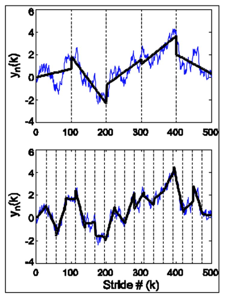
Illustration of detrended fluctuation analysis. In each figure, the blue line is the integrated stride time series and the horizontal axis is the stride number, denoted by i. Each stride interval time series was divided into 5 bins (n = 100; shown on top). A line was fit to the data in each bin using linear regression (black line). This linear fit was then subtracted from the original and the R error was calculated. This process was repeated for a variety of bins lengths between 4 and 125 (shown on bottom for bin length = 25). As bin size decreased the error also decreased.

$$F(n)=\sqrt{\frac{1}{N}\sum _{k=1}^N{[y(k)-y_{\mathit{fit}}(k)]}^2}$$ (6)

This process was repeated for different values of segment lengths, n. Fifty values of n that were evenly distributed between 4 and N/4 were used [30]. Typically, F(n) increases with n and a graph of log[F(n)] versus log(n) will exhibit a power-law relationship indicating the presence of scaling, such that F(n) ≅ n^α. These log[F(n)] versus log(n) plots were then fit with a linear function using a standard least squares regression approach. The slope of this line defined the scaling exponent α. A value of α = 0.5 indicates the stride intervals are completely uncorrelated (i.e., white noise). For this condition, the time series of the stride intervals could be rearranged in any manner (through surrogate data analysis) and DFA analysis would still produce α = 0.5. When, α < 0.5, the stride intervals contain short-range correlations. Long-range correlations are present when 0.5 < α ≤ 1.0. When α > 1.0, the time series is brown noise (i.e., integrated white noise) [1]. Higher order (i.e., quadratic) detrending was also applied, but consistent with previous findings in human gait [2], the α’s obtained did not change significantly. Therefore, all results reported are for linear detrending.

3. RESULTS

The model ran successfully for all noise conditions with A = 0 and A = 0.8. When A was increased to A = 0.9 and A = 1.0, the model became unstable at high noise levels. The variability in the system increased with applied noise. This can be seen in the phase plots for θ and φ (Fig. 3). Compared to human walking, however, the model was less variable and took significantly more time to take each stride (Fig. 4). Despite these differences, the model had the same correlation structure as seen in a previous study of healthy human subjects walking at a comfortable pace [6].

Figure 3.

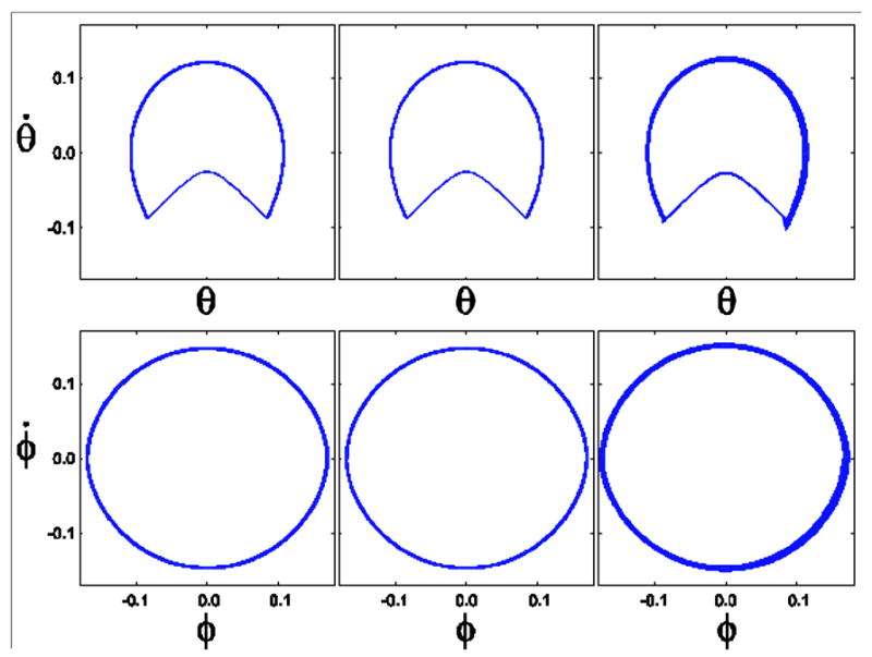
Phase plots for three different walking conditions. In each case A = 1.0. The magnitude of the noise increases from left to right. The left column shows the phase plots for low noise (ξ_S = ξ_M = 10⁻⁶), the middle column for moderate noise (ξ_S = ξ_M = 10⁻⁴), and the right column for high noise (ξ_S = ξ_M = 10⁻³). At A = 1.0, the model could not walk consistently without falling over at noise levels greater than the high noise condition shown.

Figure 4.

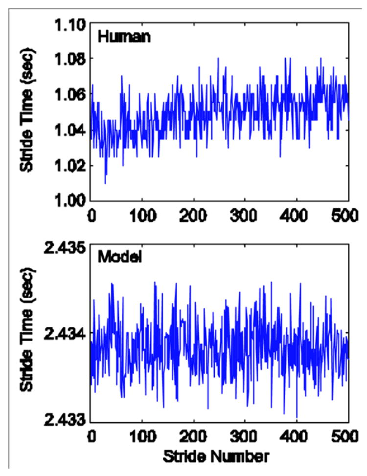
Data from a typical healthy human subject (top) [6] compared to the output from the model (bottom) walking with a moderate level of noise (A = 1.0, ξ_S = ξ_M = 10⁻⁵). Humans walk faster and with more variability than the model. However, both time series exhibited long-range correlations (a = 0.755 for both the experimental and model data).

Figures 5 and 6 show how the correlations changed as the model parameters were varied. All linear fits to the log[F(n)] versus log(n) plots had r² > 0.91 (e.g., Fig. 6, right) and were highly statistically significant (p < 0.001). In the case where A = 0, only ξ_M influenced α since ξ_S was multiplied by zero (Eq. 4). In this case, the time series exhibited short-range correlations at high noise levels (ξ_M > 10^−4.5), was uncorrelated at moderate noise levels (ξ_M ≅ 10⁻⁴), and displayed long-range correlations at very low noise levels (ξ_M < 10⁻⁴) (Fig. 5A). When A was non-zero, the plots were roughly symmetric, showing that both noise terms had an approximately equal impact on the type of correlations found in the data (Fig. 5B-D). At A = 0.8 and A = 0.9 the model produced stride time series that were short-range correlated, uncorrelated, or had long range correlations. When A was increased to A = 1.0, the model no longer produced short-range correlations. At high noise levels, the model produced time series consistent with brown noise. At higher noise levels, the model fell over before completing 1100 steps.

Figure 5.

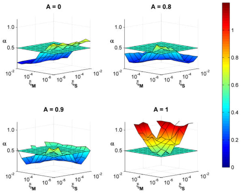
Average a values of 10 runs of the simulation for 4 values of A and 10 values of ξ_S and ξ_M. At A = 0.9 and 1.0, the model did not successfully complete all 550 strides for large values of ξ_S and ξ_M.. Results of those trials were therefore omitted. For A = 0.0, 0.8, and 0.9 the stride interval time series were predominantly anti-correlated (α < 0.5). There were narrow ranges where the series was uncorrelated (α ≈ 0.5) and then showed long-range correlations (0.5 < α < 1.0) at low noise levels. At A = 1.0, the stride interval time series exhibited long-range correlations at low noise levels, and Brownian motion (α ≈ 1.0) at high noise levels.

Figure 6.

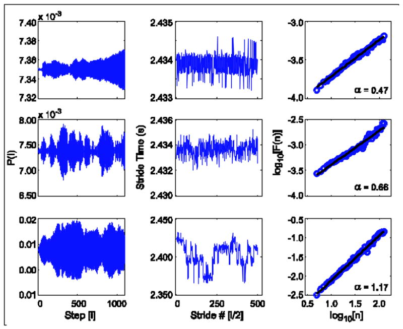
Examples of the effect of noise on the push-off impulse (P_i), stride intervals, and results of detrended fluctuation analysis for the three different sensory noise levels are shown in Figure 3. In each case, ξ_M = 10⁻⁶. From top to bottom, the conditions are A) low noise (ξ_S = 10⁻⁶), B) moderate noise (ξ_S = 10⁻⁴), and C) high noise (ξ_S =10⁻³). Note that the scales on the vertical axes vary with condition. The value of a increased with the amount of applied sensory noise. In the low noise condition, the stride interval time series was random uncorrelated noise (a = 0.47). In the moderate noise condition, the stride interval time series exhibited long-range correlations (a = 0.66) and in the high noise condition, the time series was consistent with brown noise (a = 1.17). Similar results are obtained by varying ξ_M. Thus, with the correct choice of parameters, it was possible to obtain various types of correlation from the system.

By appropriately varying the parameters, nearly any type of correlation structure could be obtained (e.g., Fig. 6). For example, in Fig. 6, A and ξ_M were held fixed at A = 1 and ξ_M = 10⁻⁶, while ξ_S was varied to show short-range correlations (low noise), long-range correlations (moderate noise) and brown noise (high noise). Similar changes were obtained by holding ξ_M fixed and varying ξ_S, or by varying ξ_M and ξ_S simultaneously (not shown). Likewise, the same type of correlation structure could be obtained for multiple different parameter combinations.

In addition to changes in α, changes in variability (i.e., standard deviations) are observed in clinical populations, independent of changes in α [3, 4, 31]. In our model, the variability of stride times increased approximately exponentially with increases in applied noise (Fig. 7) for all values of A. Consequently, there were parameter regimes where α exhibited large changes while variability changed little and regimes where variability increased dramatically, while α changed little. Thus, the changes in α observed in our model were also independent of changes in stride time variability.

Figure 7.

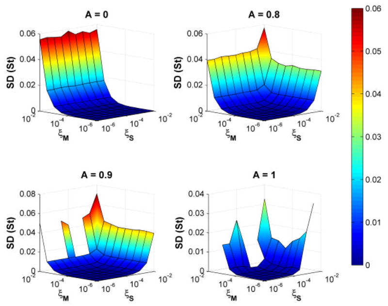
Average stride time standard deviations, SD(St), for 10 simulations each for 4 values of A and 10 values each of ξ_S and ξ_M. At A = 0.9 and 1.0, the model did not complete all 550 strides for large values of ξ_S and ξ_M, so results for those trials are not shown. For all values of A, stride time variability increased approximately exponentially with increases in ξ_S, ξ_M, or both. These changes in variability were thus independent of changes in α.

4. DISCUSSION

Long-range correlations have been observed in the stride intervals of human walking [1, 32, 33] and these correlations change with various experimental interventions [2] and/or disease processes affecting the central nervous system [4, 5]. Previous modeling efforts conducted to explain these experimental results have focused on properties of complex supra-spinal neural control mechanisms [1, 7, 8]. While these models appear promising, they do not exclude other, possibly simpler explanations. In particular, it has also previously been shown that the complex movement patterns humans exhibit during quiet standing [12, 13] can be replicated by a relatively simple biomechanical model [21]. The present study was therefore conducted to test the hypothesis that long-range correlations in stride intervals could also be obtained from a simple biomechanical model of bipedal walking operating under minimal feedback (e.g., spinal reflex) control.

The results of the detrended fluctuation analyses of the stride interval time series generated by the model (Figs. 5 & 6) supported this hypothesis. With appropriate parameter choices, the model exhibited a wide range of different correlation structures, including short-range and long-range correlations, and Brownian motion. These solutions were also not unique, in that the same type of correlation structures were obtained using a variety of parameter values. Even when no noise was included in our simulations, the model still exhibited very small amounts of variability and long-range correlations (α > 0.5). This was likely due at least in part to the inherent nonlinearities in the model and the discontinuities introduced by the instantaneous switching between the legs at foot-strike (Eq. 3). Also, slight inaccuracies in numerical computations due to the inherent limitations in floating-point precision that always occur when running such simulations on digital computers also contributed to these “noise free” variations.

Likewise, we also found long-range correlations even in the complete absence of feedback control (Fig. 5; A = 0 case). While these simulations did incorporate white noise as “motor output” noise (Eq. 4), white noise alone can neither account for, nor create, long-range correlations. Thus, these long-range correlations had to come from the interaction of this white noise with the mechanical system. Also, while we described this noise as “motor output” noise (which could come from the central or peripheral nervous systems, and/or the muscular system), we could have obtained the same result by applying external (i.e., environmental) noise (e.g., by having the model walk over an irregular surface) to a walking model incorporating both no neural feedback (A = 0) and no biological noise sources. Together, these results demonstrate that long-range correlations can occur in bipedal walking in the absence of complex central nervous system control. Thus, supra-spinal control mechanisms may not be as “essential” for generating complex stride interval time series as previously suggested [34]. These correlations may instead result from the interactions of noisy neural signals trying to control a highly nonlinear biomechanical structure.

This simple model of bipedal gait reproduced several experimental findings (e.g., [1, 4, 35]) exhibiting either the presence or loss of long-range correlations for different patient groups and/or experimental manipulations. However, our results suggest alternative possible explanations for the mechanisms causing these changes. For example, in the elderly, stride intervals become uncorrelated [4]. One reason this may occur is an increase in motor output noise. As people age, the number of motor units within a muscle decreases [36]. Since the number of muscle fibers is also reduced, larger motor units are substituted for small ones [37]. This results in a loss of the ability to perform finely controlled movements. The resulting loss of long-range correlations with increased motor output noise is completely consistent with the results of our model: as shown in Figure 5, for 0.0 ≤ A ≤ 0.9, as motor output noise (ξ_M) increased, a decreased. Our model also showed that changes in either ‘sensory’ or ‘motor’ noise each yielded approximately the same result, suggesting that noise present at any point in the system can ultimately affect changes in these stride time correlations.

It should be noted that the model presented here is highly simplistic and as such does not replicate many important aspects of human walking. As such, we cannot directly relate the values of the model coefficients (e.g., A, ξ_S, ξ_M, etc.) to any specific individual physiological parameters or mechanisms. Also, the stable basin of attraction of our model was extremely small [38] since it incorporated only a minimal control system. As such, the minimum perturbations required to cause our model to fall were much smaller than would be expected for humans. Thus, the magnitude of the variability exhibited by our model was much less than that typically observed in humans (Fig. 4). However, humans have many more feedback mechanisms (visual, vestibular, proprioception, etc.) they can use to help them accommodate a much wider range of perturbations. Adding such additional feedback to our model would significantly increase the size of its basin of attraction [39] and therefore also the range of stride time variations the model could exhibit before falling over. However, we believe we would still be able to observe the same qualitative changes in α found here for such a model. Finally, our model also walked much slower than typical humans because leg swing was limited to the harmonic frequency of the pendulum [23]. Humans have muscles to help actively propel them forward. Adding additional power for forward propulsion to the model would significantly increase its walking speed [40].

These limitations not withstanding, simple biomechanical models like the one used here do successfully predict several fundamental features of human walking, including the preferred speed–step length relationship [41], as well as several important aspects related to locomotor energetics [25, 42] and locomotor stability [43]. The results of the present study suggest that the long-range correlations observed in locomotor stride times might be added to the list of fundamental properties of human walking that can be explained by these simple models. While the magnitudes of the stride times for our model were much greater than humans and the amplitudes of the variations from stride to stride much less (Fig. 4), the correlation structure (i.e., the temporal scaling) observed in these stride interval time series were the same. Thus, while our model does not completely replicate human walking, it does show that even the basic mechanics of walking can produce fractal-like behavior. It is therefore likely that these same basic features would also be seen in more complex models of bipedal walking.

In summary, healthy humans exhibit long-range correlations in their stride times [1, 2]. These correlations degrade with central nervous system disorders [4, 5] and increase with stressors [2], suggesting that central processing is vital for regulating these aspects of gait cycle timing [1, 7, 8]. The results of this study demonstrate that the long-range correlations observed in the stride interval time series of human walking might be due instead to the inherent biomechanical structure of the system and may not require complex central nervous system control mechanisms. Previous models that have focused on properties of the central nervous system to explain the origins of these fractal-like features of gait cycle timing [1, 7, 8] cannot preclude the possibility that these features arise instead from the inherent biomechanics of the locomotor system. Likewise, it is equally true that the model proposed here cannot entirely preclude the possibility that the central nervous system still plays a significant role in regulating these processes. Because of its simplicity, some of the clinical changes observed n humans are difficult to interpret with our current model. Therefore, future work must focus on determining precisely how both central nervous system processes and biomechanical factors contribute to these observed phenomena.

References

- 1.Hausdorff JM, Peng CK, Ladin Z, Wei JY, Goldberger AL. Is Walking a Random Walk? Evidence for Long-Range Correlations in Stride Interval of Human Gait. J Appl Physiol. 1995;78(1):349–358. doi: 10.1152/jappl.1995.78.1.349. [DOI] [PubMed] [Google Scholar]
- 2.Hausdorff JM, Purdon PL, Peng CK, Ladin Z, Wei JY, Goldberger AL. Fractal Dynamics of Gait: Stability of Long-Range Correlations in Stride Interval Fluctuations. J Appl Physiol. 1996;80(5):1448–1457. doi: 10.1152/jappl.1996.80.5.1448. [DOI] [PubMed] [Google Scholar]
- 3.Goldberger AL, Amaral LAN, Hausdorff JM, Ivanov PC, Peng CK, Stanley HE. Fractal Dynamics in Physiology: Alterations with Disease and Aging. Proc Natl Acad Sci USA. 2002;99(Suppl 1):2466–2472. doi: 10.1073/pnas.012579499. [DOI] [PMC free article] [PubMed] [Google Scholar]
- 4.Hausdorff JM, Mitchell SL, Firtion R, Peng CK, Cudkowicz ME, Wei JY, Goldberger AL. Altered Fractal Dynamics of Gait: Reduced Stride Interval Correlations with Aging and Huntington's Disease. J Appl Physiol. 1997;82(1):262–269. doi: 10.1152/jappl.1997.82.1.262. [DOI] [PubMed] [Google Scholar]
- 5.Frenkel-Toledo S, Giladi N, Peretz C, Herman T, Gruendlinger L, Hausdorff JM. Treadmill walking as an external pacemaker to improve gait rhythm and stability in Parkinson's disease. Mov Disord. 2005;20(9):1109–14. doi: 10.1002/mds.20507. [DOI] [PubMed] [Google Scholar]
- 6.Gates DH, Dingwell JB. Peripheral Neuropathy Does Not Alter the Fractal Dynamics of Gait Stride Intervals. J Appl Physiol. doi: 10.1152/japplphysiol.00413.2006. In Revision. [DOI] [PMC free article] [PubMed] [Google Scholar]
- 7.Ashkenazy Y, Hausdorff JM, Ivanov PC, Stanley HE. A stochastic model of human gait dynamics. Physica A. 2002;316(1–4):662–670. [Google Scholar]
- 8.West BJ, Scafetta N. Nonlinear dynamical model of human gait. Phys Rev E. 2003;67(5):051917. doi: 10.1103/PhysRevE.67.051917. [DOI] [PubMed] [Google Scholar]
- 9.West B, Latka M. Fractional Langevin model of gait variability. J NeuroEng Rehabil. 2005;2(1):24. doi: 10.1186/1743-0003-2-24. [DOI] [PMC free article] [PubMed] [Google Scholar]
- 10.Smethurst DP, Williams HC. Power Laws: Are Hospital Waiting Lists Self-Regulating? Nature. 2001;410(6829):652–653. doi: 10.1038/35070647. [DOI] [PubMed] [Google Scholar]
- 11.Freckleton RP, Sutherland WJ. Hospital Waiting-Lists (Communication Arising): Do Power Laws Imply Self-Regulation? Nature. 2001;413(6854):382. doi: 10.1038/35096646. [DOI] [PubMed] [Google Scholar]
- 12.Collins JJ, DeLuca CJ. Open-Loop and Closed-Loop Control of Posture: A Random-Walk Analysis of Center-of-Pressure Trajectories. Exp Brain Res. 1993;95:308–318. doi: 10.1007/BF00229788. [DOI] [PubMed] [Google Scholar]
- 13.Collins JJ, DeLuca CJ. Random Walking During Quiet Standing. Phys Rev Let. 1994;73(5):764–767. doi: 10.1103/PhysRevLett.73.764. [DOI] [PubMed] [Google Scholar]
- 14.Collins JJ, DeLuca CJ. The Effects of Visual Input on Open-Loop and Closed-Loop Postural Control Mechanisms. Exp Brain Res. 1995;103(1):151–163. doi: 10.1007/BF00241972. [DOI] [PubMed] [Google Scholar]
- 15.Riley MA, Balasubramaniam R, Turvey MT. Common Effects of Touch and Vision on Postural Parameters. Exp Brain Res. 1997;117(1):165–170. doi: 10.1007/s002210050211. [DOI] [PubMed] [Google Scholar]
- 16.Collins JJ, DeLuca CJ, Burrows A, Lipsitz LA. Age-Related Changes in Open-Loop and Closed-Loop Postural Control Mechanisms. Exp Brain Res. 1995;104(3):480–492. doi: 10.1007/BF00231982. [DOI] [PubMed] [Google Scholar]
- 17.Mitchell SL, Collins JJ, DeLuca CJ, Burrows A, Lipsitz LA. Open-Loop and Closed-Loop Postural Control Mechanisms in Parkinson's Disease: Increased Mediolateral Activity During Quiet Standing. Neurosci Lett. 1995;197:133–136. doi: 10.1016/0304-3940(95)11924-l. [DOI] [PubMed] [Google Scholar]
- 18.Chow CC, Collins JJ. Pinned Polymer Model of Posture Control. Phys Rev E. 1995;52(1):907–912. doi: 10.1103/physreve.52.907. [DOI] [PubMed] [Google Scholar]
- 19.Lauk M, Chow CC, Pavlik AE, Collins JJ. Human Equilibrium Out of Balance: Nonequilibrium Statistical Mechanics in Postural Control. Phys Rev Let. 1998;80(2):413–416. [Google Scholar]
- 20.Chow CC, Lauk M, Collins JJ. The dynamics of quasi-static posture control. Hum Mov Sci. 1999;18(5):725–740. [Google Scholar]
- 21.Peterka RJ. Postural Control Model Interpretation of Stabilogram Diffusion Analysis. Biol Cybern. 2000;82(4):308–318. doi: 10.1007/s004220050587. [DOI] [PubMed] [Google Scholar]
- 22.Hausdorff JM, Peng CK. Multiscaled randomness: A possible source of 1/f noise in biology. Phys Rev E. 1996;54(2):2154. doi: 10.1103/physreve.54.2154. [DOI] [PubMed] [Google Scholar]
- 23.Garcia M, Chatterjee A, Ruina A, Coleman M. The Simplest Walking Model: Stability, Complexity, and Scaling. J Biomech Eng. 1998;120(2):281–288. doi: 10.1115/1.2798313. [DOI] [PubMed] [Google Scholar]
- 24.McGeer T. Passive Dynamic Walking. Int J Robot Res. 1990;9(2):68–82. [Google Scholar]
- 25.Kuo AD, Donelan JM, Ruina A. Energetic Consequences of Walking Like an Inverted Pendulum: Step-to-Step Transitions. Exerc Sport Sci Rev. 2005;33(2):88–97. doi: 10.1097/00003677-200504000-00006. [DOI] [PubMed] [Google Scholar]
- 26.Kuo AD. Energetics of actively powered locomotion using the simplest walking model. J Biomech Eng. 2002;124(1):113–120. doi: 10.1115/1.1427703. [DOI] [PubMed] [Google Scholar]
- 27.Peng CK, Buldyrev SV, Goldberger AL, Havlin S, Simons M, Stanley HE. Finite size effects on long-range correlations: implications for analyzing DNA sequences. Phys Rev E. 1993;47:3730–3733. doi: 10.1103/physreve.47.3730. [DOI] [PubMed] [Google Scholar]
- 28.Peng CK, Buldyrev SV, Hausdorff JM, Havlin S, Mietus JE, Simons M, Stanley HE, Goldberger AL. Non-Equilibrium Dynamics as an Indispensable Characteristic of a Healthy Biological System. Integr Physiol Behav Sci. 1994;29(3):283–293. doi: 10.1007/BF02691332. [DOI] [PubMed] [Google Scholar]
- 29.Peng CK, Buldyrev SV, Havlin S, Simons M, Stanley HE, Goldberger AL. Mosaic Organization of DNA Nucleotides. Phys Rev E. 1994;49(2):1685–1689. doi: 10.1103/physreve.49.1685. [DOI] [PubMed] [Google Scholar]
- 30.Jordan K, Challis JH, Newell KM. Long range correlations in the stride interval of running. Gait Posture. 2006;24(1):120–125. doi: 10.1016/j.gaitpost.2005.08.003. [DOI] [PubMed] [Google Scholar]
- 31.Malatesta D, Simar D, Dauvilliers Y, Candau R, Borrani F, Prefaut C, Caillaud C. Energy cost of walking and gait instability in healthy 65- and 80-yr-olds. J Appl Physiol. 2003;95(6):2248–2256. doi: 10.1152/japplphysiol.01106.2002. [DOI] [PubMed] [Google Scholar]
- 32.West BJ, Griffin L. Allometric Control of Human Gait. Fractals. 1998;6(2):101–108. [Google Scholar]
- 33.West BJ, Griffin L. Allometric Control, Inverse Power Laws and Human Gait. Chaos, Solitons, & Fractals. 1999;10(9):1519–1527. [Google Scholar]
- 34.Costa M, Peng CK, Goldberger AL, Hausdorff JM. Multiscale entropy analysis of human gait dynamics. Physica A. 2003;330(1–2):53–60. doi: 10.1016/j.physa.2003.08.022. [DOI] [PMC free article] [PubMed] [Google Scholar]
- 35.Hausdorff JM, Zemany L, Peng CK, Goldberger AL. Maturation of Gait Dynamics: Stride-to-Stride Variability and its Temporal Organization in Children. J Appl Physiol. 1999;86(3):1040–1047. doi: 10.1152/jappl.1999.86.3.1040. [DOI] [PubMed] [Google Scholar]
- 36.Challis JH. Aging, regularity and variability in maximum isometric moments. J Biomech. 2006;39(8):1543–1546. doi: 10.1016/j.jbiomech.2005.04.008. [DOI] [PubMed] [Google Scholar]
- 37.Darling WG, Cooke JD, Brown SH. Control of simple arm movements in elderly humans. Neurobiol Aging. 1989;10(2):149–157. doi: 10.1016/0197-4580(89)90024-9. [DOI] [PubMed] [Google Scholar]
- 38.Schwab AL, Wisse M. Basin of attraction of the simplest walking model. Paper # DETC01/VIB-21363; Proceedings of the 2001 ASME Design Engineering Technical Conferences and Computers and Information in Engineering Conference; Pittsburgh, PA. 2001. [Google Scholar]
- 39.Wisse M, Schwab AL, Linde RQvd, Helm FCTvd. How to Keep From Falling Forward: Elementary Swing Leg Action for Passive Dynamic Walkers. IEEE Trans Robot. 2005;21(3):393–401. [Google Scholar]
- 40.Collins SH, Ruina A, Tedrake R, Wisse M. Efficient Bipedal Robots Based on Passive-Dynamic Walkers. Science. 2005;307(5712):1082–1085. doi: 10.1126/science.1107799. [DOI] [PubMed] [Google Scholar]
- 41.Kuo AD. A Simple Model of Bipedal Walking Predicts the Preferred Speed-Step Length Relationship. J Biomech Eng. 2001;123(3):264–269. doi: 10.1115/1.1372322. [DOI] [PubMed] [Google Scholar]
- 42.Donelan JM, Kram R, Kuo AD. Mechanical work for step-to-step transitions is a major determinant of the metabolic cost of human walking. J Exp Biol. 2002;205(23):3717–3727. doi: 10.1242/jeb.205.23.3717. [DOI] [PubMed] [Google Scholar]
- 43.Donelan JM, Shipman DW, Kram R, Kuo AD. Mechanical and metabolic requirements for active lateral stabilization in human walking. J Biomech. 2004;37(6):827–835. doi: 10.1016/j.jbiomech.2003.06.002. [DOI] [PubMed] [Google Scholar]