Imaging large scale neural activity with cellular resolution in awake mobile mice

Abstract

We report a technique for two-photon fluorescence imaging with cellular resolution in awake behaving mice with minimal motion artifact. The apparatus combines an upright table mounted two-photon microscope with a spherical treadmill consisting of a large air supported Styrofoam ball. Mice, with implanted cranial windows, are head restrained under the objective while their limbs rest on the ball’s upper surface. Following adaptation to head restraint, mice maneuver on the spherical treadmill as their head remains motionless. Image sequences demonstrate that running-associated brain motion is limited to ~2–5 µm. In addition, motion is predominantly in the focal plane, with little out-of-plane motion, making the application of a custom designed Hidden Markov Model based motion correction algorithm useful for post-processing. Behaviorally correlated calcium transients from large neuronal and astrocytic populations were routinely measured, with an estimated motion induced false positive error rate of <5%.

Introduction

Existing methods for mammalian brain imaging have either been difficult to apply to awake animals or lack the cellular resolution necessary for characterizing neural circuits. Wide-field CCD imaging has revealed large scale activity patterns in response to whisker stimuli in freely moving mice (Ferezou et al., 2006), but provides little depth penetration into brain tissue, no capacity for optical sectioning, and spatial resolution an order of magnitude too low for single cell studies. Two-photon microscopy (TPM) (Denk et al., 1990; Denk and Svoboda, 1997) overcomes many of these restrictions and mouse in vivo studies have allowed for tracing learning dependent dendritic spine morphology (Holtmaat et al., 2006; Holtmaat et al., 2005), recording the biochemical signals associated with dendritic excitability (Helmchen et al., 1999; Svoboda et al., 1997) and tracking the activity of hundreds of neurons simultaneously (Ohki et al., 2005). However, because high-resolution imaging requires mechanical stability, all previous in vivo mouse TPM studies have used anesthetized preparations. Anesthesia greatly reduces overall brain activity (Berg-Johnsen and Langmoen, 1992) and completely abolishes or alters several forms of neural dynamics, such as persistent activity (Major and Tank, 2004). Currently, the chief impediment for TPM in awake behaving mice is the relative motion between the brain and microscope typically associated with animal movements.

There are two general approaches for TPM in awake mice: head mounted microscopes and head-restraint. A head mounted microscope requires innovative engineering to miniaturize the excitation, laser scanning and fluorescence collection. One such device demonstrated stable TPM of capillaries in awake and resting adult rats (Helmchen et al., 2001); however, because it was not optimized for moving animals, relative motion between the microscope and brain was apparent during animal movements. An even smaller device has been reported (Flusberg et al., 2005), but its use in awake behaving mice has not been demonstrated. As an alternative to a head-mounted miniaturized microscope, head restrained TPM may be possible using a standard microscope design. Little research has been directed toward head-restrained TPM in the awake mouse, possibly because there are concerns over the induction of stress, or that the animal’s increased leverage would cause torques leading to large relative movements between the microscope and brain.

The imaging technique we developed uses head restraint, but employs an air supported spherical treadmill to allow walking and running. The treadmill was adapted from insect studies (Dahmen, 1980; Mason et al., 2001; Stevenson et al., 2005) and was previously used to stably record head direction cell activity for hours in head fixed mice using chronically implanted microelectrodes (Khabbaz and Tank, 2004). We demonstrate that TPM image sequences at cellular resolution can be collected with relatively little frame to frame displacement and within-frame distortion due to brain motion. Furthermore, residual in plane motion can be corrected using a Hidden Markov Model (HMM) algorithm. Our approach allows for imaging of cellular resolution calcium dynamics in neural and astrocytic populations in behaving mice.

Results

Apparatus and animal behavior

Our strategy is based on a two photon-microscope built around a spherical treadmill constructed from an air supported, 8-inch diameter Styrofoam ball (Figure 1A). The animal can run freely in two-dimensions on the upper surface of the ball while the skull is held rigidly in place with respect to the microscope objective. The frictionless movement of the treadmill reduces possible head torques the animal can apply and thus relative motion between the brain and microscope is potentially reduced. To record ball rotation produced by walking and running, two optical computer mice were positioned along the equator of the spherical treadmill 90° apart. Detected motion signals were computer recorded and synchronized in time with image sequence acquisition. An infrared CCD camera was used for observing whisking and grooming.

Figure 1.

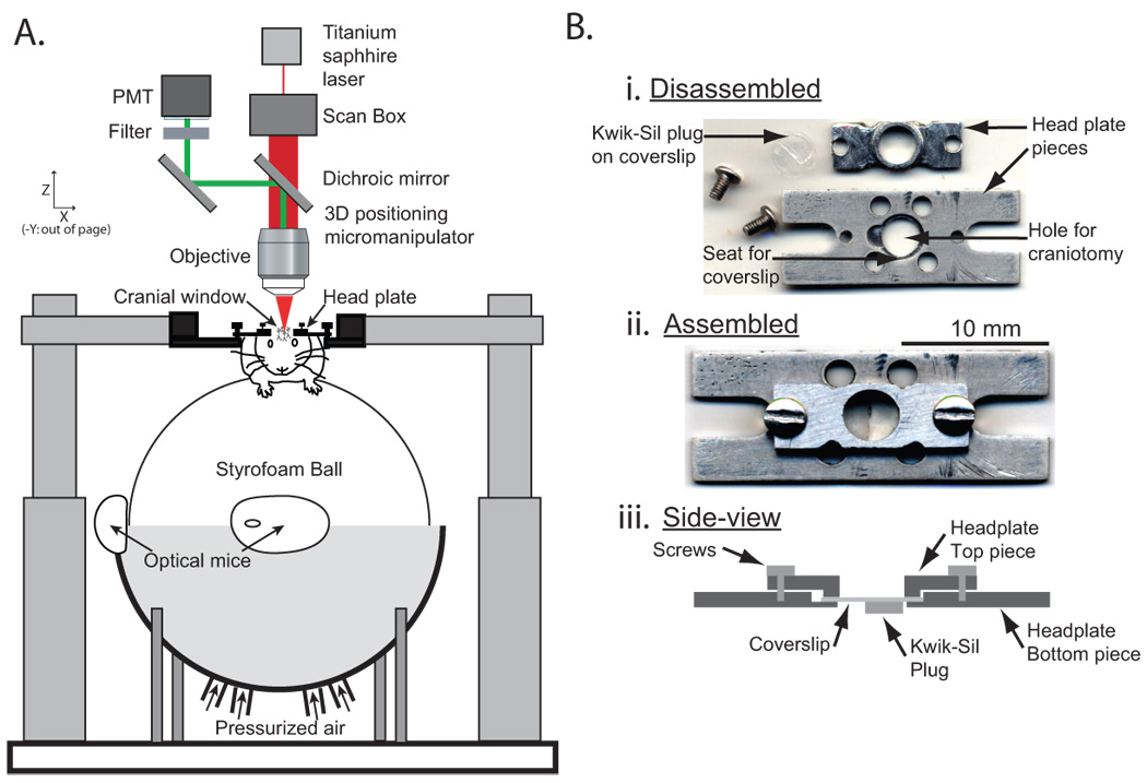
Awake mouse two-photon microscopy experimental apparatus. A) A two-photon microscope is used to image through the cranial window of an awake behaving mouse that is able to maneuver on an air-supported free-floating Styrofoam ball that acts as a spherical treadmill. Optical computer mice are used to record mouse locomotion by quantifying treadmill movement. B) Images of the disassembled (i) and assembled (top-view (ii) and side-view (iii)) head-plate used for cranial window imaging and mouse head restraint.

Adapting the mice to the head-restrained treadmill consisted of three sessions totaling ~1 hour (See methods). By the end of the third session, mice walked, ran and rested on the treadmill and showed no signs of struggling against the head restraint; in addition, most animals displayed grooming behavior (see online Supplemental Movie 1). Running activity was quantified (n=7 mice) in terms of mean distance run per hour (236+/−72 m), time spent running (34+/−8%), and speed while running (0.13+/−0.003 m/s). These values were within the range seen during conventional exercise wheel running for isolated caged mice with free wheel access (Turner et al., 2005).

Two-photon imaging in mobile mice

We implanted custom designed head plates and cranial windows in adult Thy1.2 YFP mice (Feng et al., 2000) and 5–7 week old adolescent wild type (WT) mice. The head plate design consisted of a two-piece, 1 gram titanium assembly (Figure 1B). The larger piece, containing a ~4 mm diameter hole with a recessed seat for a cover slip to sit in, was permanently affixed to the skull with the hole centered over the brain region to be imaged; the second smaller piece could be clamped with screws onto the first piece to rigidly hold a cover slip in place. The void in the craniotomy between the dura surface and the cover slip was filled with a pre-molded plug of Kwik-Sil (Figure 1B). The uniform thickness of the plug was chosen so that it applied slight pressure to the surface of the dura when the clamping plate was installed; when in place, the plug pushed the brain surface ~100–200 µm below the bottom edge of the skull. The dura was allowed to dry until tacky before the plug was implanted; this resulted in greater contact friction between the dura and plug and reduced brain motion.

After spherical treadmill training and head plate installation, the brain area within the craniotomy could be routinely imaged by TPM in awake mice. To characterize our imaging technique, image sequences of cortical neurons expressing YFP in adult mice and cortical astrocytes highlighted with the dye Sulforhodamine 101 (SR101) in younger WT adolescent mice were collected during resting, walking and running. Image sequences, shown in Figures 2A,C (time-series of YFP and SR101 in online Supplemental Movie 2 and Supplemental Movie 3, respectively), showed little frame to frame distortion during the resting state. During running, there were small movement-related lateral displacements of ~3–5 µm for adult YFP and ~2–3 µm for adolescent WT mice (see shifts relative to cross-hairs in Figures 2A, C). In addition, there was very little out of plane (Z direction) brain motion: small scale structures typically remained in focus during the entire imaging sequence. Although functional imaging experiments could be performed with this unprocessed data (see Supplemental Figure 1), residual lateral shifts could be corrected in order to both quantify brain motions and further reduce image distortions.

Figure 2.

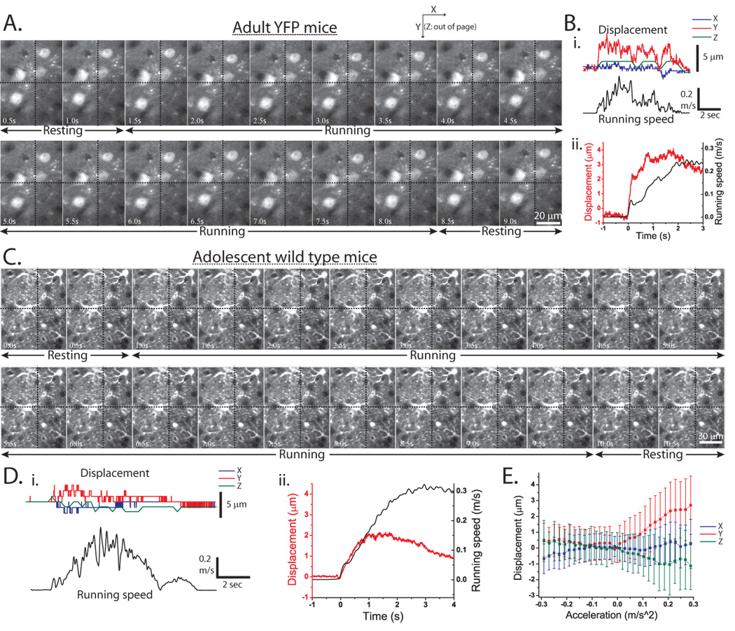
Image sequences and quantification of brain motion caused by mouse movements. A,C) Frames from a two-photon time-series (unprocessed data, no motion correction) of YFP expressing cortical neurons in adult YFP (A, ~200 µm deep) and SR101 labeled cortical astrocytes in adolescent WT (C, ~200 µm deep) mice during periods of resting and running. The three components (X,Y and Z) of brain motion (displacement) were quantified and coplotted with running speed for YFP (Bi) and WT (Di) mice. Note that individual astrocytic processes can be followed in all frames of C. Larger amplitude brain motion can be seen in YFP mice in a running onset triggered average of Y-displacement (Bii) compared to the smaller amplitude brain motion seen in a running triggered y-displacement average for younger WT mice (Dii). E) A plot of brain motion versus running acceleration for WT mice. Positive mouse running accelerations lead to the largest brain displacements, while little displacement is seen during deceleration or constant running velocity.

Motion correction

Our strategy to quantify in focal plane brain motion was to correct frames back to a reference image selected from the resting state using an offline line-by-line algorithm (Figure 3) based on a HMM (Rabiner, 1989). As illustrated in Figure 3A, relative motion of the brain with respect to the microscope during the raster scanned progression of the focused beam across the sample replaces an expected line in the image with a line of pixels from the sample at an X- and Y-shifted location. The appropriate correction is to remap the recorded line by placing it at the corresponding X and Y shifted location in a reconstructed image. The HMM model uses a maximum likelihood method to determine which X- and Y- shifted position (displacements) of the image is the most probable, by finding the most probable sequence of brain movement offsets for the successive lines acquired in the time-series (Figure 3Di). The probability of a given sequence of offsets is a function of two components, summed over all time points in the sequence: 1. The fit of the line scanned at a given time point compared to the reference image at the offset given, 2. The probability of the offset transitioning from the offset given at the previous time point, to the current offset. The fit was based upon Poisson statistics of photon counting (Figure 3Diii) and the probability of a transition in offset was modeled as a spatially invariant exponential relation, whose space constant was determined by expectation maximization (Figure 3Dii) (see methods for more details). Tests on simulated image sequences produced by distorting a real image using a known sequence of movements (Figure 3B) directly demonstrate the ability of the algorithm to predict the true displacement of the sample (Figure 3C) and produce a spatially undistorted image (Figure 3Biii). The results of motion correction on real time-series data can be seen in Supplemental Movie 2 and Supplemental Movie 3.

Figure 3.

Motion Correction using a Hidden Markov Model. A) A simplified demonstration of the corruption created by a sample moving during frame acquisition by laser scanning microscopy. i) The first half of the frame is acquired with the sample held fixed at one position. After the green line is scanned, the sample makes a sudden movement. ii) The second half of the frame is acquired with the sample displaced. iii) A reference image of the sample as it would have been acquired with no displacements. iv) An image as it would have been acquired if the sample had undergone the displacement as indicated between i and ii. Lines between images indicate the relative Y position of line scans. B) Simulation of laser scanning microscopy of a sample undergoing continuous motion displacement. Blue lines between sample (i) and simulated data (ii) indicate mean Y position of each line scan. Partial reconstruction (iii) of the sample is possible by estimating the relative position of each line to the standard raster scanning pattern. Red lines between simulated data and reconstruction indicate the prediction of a HMM of the Y position of each line scan. There are sections of sample over which the beam did not pass, and so blank lines are an unavoidable result of brain motion causing non-uniform spatial sampling C) Displacements of the sample during the simulated frame acquisition. Actual displacements are indicated in red and black. Displacements predicted by the algorithm are shown in blue and green and are slightly vertically offset for clarity. D) i) Two hypothetical examples of sequences of offsets considered in the HMM model. Transitions between offsets are indicated with arrows colored with respect to the exponential model illustrated in ii. The circles at each offset position have been colored with respect to the fit of the line to the sample at that offset, as illustrated in iii. Although the fit at 4a is the most probable offset for line 4, the path through 4b is more probable because it has smaller incremental offsets. ii) Illustration of the exponential model of the probability of a transition in offset from one line to the next. Probabilities shown here are for a space constant λ=0.5, which produced the overall most probable prediction shown in C. iii) Relative fit of line 40 to the sample over a range of offsets.

Quantifying brain motion

X and Y displacements calculated by the motion correction algorithm were used as a metric for quantifying in plane brain motion. Out of plane motion (Z-direction) was determined by comparing a region of each frame in the time-series to a Z-series image stack obtained above and below the time-series acquisition plane to find the plane of maximal correlation. A typical example and quantification of brain motion induced by movement in adult YFP (Figure 2Bi) and adolescent WT (Figure 2Di) mice is shown in Figure 2 along with the pooled brain motion averaged across all YFP (n=3) (Figure 2Bii) and all adolescent WT mice (n=7) (Figure 2Dii,E). In general, the average out of plane (Z) motion was on the order of the axial point spread function radius (~2 µm (Sato et al., 2007)) and much less than the in plane motion for both classes of mice. The quantitative results of the motion analysis are consistent with the qualitative observations of quite limited brain motion evident by visual inspection of the image sequences: maximum in plane brain motion seen in the younger WT mice (Figure 2D) was ~2–3 µm, while in adult YFP mice it was greater (~3–5 µm) but still relatively modest. In adolescent WT mice the displacements were well correlated with positive acceleration of running (Figure 2Dii,E). In both classes, medial-lateral (x axis) in plane motion was found to be smaller than rostral-caudal (y axis) in plane motion. One possible explanation for this difference is the symmetry of the forces on the brain in the medial-lateral direction compared to the asymmetry in the rostral-caudal direction, with skull on one side and spinal cord exerting force, on the other (Britt and Rossi, 1982). Though frame to frame out-of-plane motion was typically low (~1 µm) slow drifts were often observed over the course of 4–5 minute recordings; these changes were relatively small (0.6+/−0.5 µm/min) and rarely inhibited acquisition or analysis of functional or structural data.

Relative brain and skull motion was compared by imaging fluorescent neurons in the cortex and intrinsic fluorescence from the skull. We found similar motion of both structures in young WT mice (in plane standard deviation of y-motion of 0.9+/−0.8 µm for brain and 0.7+/−0.6 µm for skull, p=0.85), but statistically less skull compared to brain motion in older YFP mice (1.7+/−0.3 µm for brain and 0.6+/−0.3 µm for skull, p=0.008). This indicates that the brain motion observed while imaging older YFP mice likely stem from the brain moving inside the more stable skull with respect to the microscope, while for younger WT mice, either the skull/brain unit or independent but comparable skull and brain motion contribute to the observed displacements during imaging.

Imaging behaviorally correlated neural activity

The usefulness of the spherical treadmill microscope system for functional imaging was tested by imaging experiments following the loading of large populations of neurons in Hind Limb Sensory Cortex (S1HL) (identified stereotactically, see Methods) with the green calcium sensitive dye Calcium Green-1-AM using multicell bolus loading (Stosiek et al., 2003). The red fluorescent dye SR101 was simultaneously injected in order to label astrocytes (Nimmerjahn et al., 2004) and provide a static, non-cell-activity dependent channel on which to apply the motion correction algorithm. Injections were performed immediately following implantation of the head plate.

A typical calcium sensitive dye recording is illustrated in Figure 4. Imaging was performed in layer 2/3, which contained many fluorescently labeled neurons and astrocytes (Figure 4Ai). An image time series (see Supplemental Movie 4) associated with this region was collected (0.256 sec/frame) after the animal awoke from anesthesia and during voluntary running and resting behavior along with stimulated running induced by air puff stimuli to the contralateral trunk and limbs. The fluorescence over time for the neuropil and numbered neuronal soma regions of interest (ROIs) indicated in Figure 4Aii is plotted in Figure 4B along with the running speed, stimulus timing and brain motion. This time series was motion corrected as described above (see Supplemental Figure 1 for a comparison of the unprocessed and corrected fluorescence traces). Nearly every neuron showed transient fluorescence increases, corresponding to increased free calcium ion concentration, during this time series. The transients of 4 of the neurons almost exactly mimic the time-course of running speed (Neurons 1, 2, 3 and 4 in Figure 4B): increased fluorescence during periods of running and a constant baseline level with reduced frequency of transients during periods of resting. In addition, many neurons (i.e. 17, 26, 27 and 28) show more sparse, but still significant, fluorescence transients that are not visibly linked to mouse running. An expanded view of 4 neurons is shown in Figure 4C. The correlation of fluorescence changes to behavior was quantified by computing the cross-correlation coefficient (C) between the fluorescence and running traces (Figure 4D). A wide range of correlations was observed: a significant fraction of the neurons showed strong running correlation (neurons 1–11, C>0.5), while others showed some (neurons 12–19, 0.5>C>0.3) or little (neurons 20–34, 0.3>C>0) correlation. The running related activity of neurons from these different correlation groups can also be seen in the form of running onset triggered fluorescence averages (Figure 4E). Interestingly, neuron 10 showed a ~1 second onset delayed response compared to running onset. As with many of the neurons, the neuropil fluorescence transients were also strongly running correlated (C of 0.6); however, the neuropil transients were many times smaller than the typical neuronal transients, ~2–5% vs. ~15–30% ΔF/F respectively. In addition to neuron-running correlations, neuron-neuron correlations were also computed (Figure 4F). In general, neurons highly, moderately, or weakly correlated with running were also highly, moderately or weakly correlated with each other, respectively. In a few specific cases, this generality did not hold; for example, while neurons 4 and 10 are strongly running correlated, their mutual fluorescence activity correlation was only moderately correlated (C of 0.4) and while neurons 31 and 32 are weakly running correlated, their activity was correlated with a C of 0.46.

Figure 4.

Imaging neural population activity in sensory cortex of awake behaving mice. Ai) False color time-projection image of the 5 minute long time series (~150 µm deep); neurons were loaded with Calcium Green-AM (green channel) and were negative for the astrocytic marker SR101 (red channel). B) Fluorescence traces for the neuropil and 34 neurons outlined in Aii obtained after the time series was motion corrected. Running speed, air puff stimulus and brain displacements are also shown. Red segments indicate >3σ positive going fluorescence transients with <5% false positive error rate (Figure 6E). C) An expanded view of the fluorescence activity of 4 neurons. D) Correlation coefficients of neuron fluorescence versus running speed. The neurons were numbered throughout this figure in descending correlation coefficient order. E) Running onset triggered average of fluorescence for 7 neurons with varying amounts of running correlation. F) Neuron-Neuron fluorescence activity correlation coefficients.

It was feasible to record image time series, such as the one shown in Figure 4, for hours. Recordings with similar signal-to-noise (S/N), brain motion, neural activity and staining were obtained in all mice (n=7 mice, 13+/−4 time series per mouse, 34+/−20 neurons per time series) (see Supplemental Movie 5 and Supplemental Movie 6, Supplemental Figure 4 and Supplemental Figure 5). Time-series movies simultaneously tracking the activity of >100 neurons were possible (Supplementary Movie 6 and Supplementary Figure 5). Running correlated neuronal and neuropil activity was observed in every mouse (on average, 16+/−16% and 53+/−38% of neurons and neuropil regions respectively with C >0.5, 31+/−15% and 27+/−23% with 0.5> C >0.3 and 53+/−28% and 19+/−20% with 0.3> C >0).

In order to show that basic properties of calcium transients we measured were similar to those observed in anesthetized preparations (Kerr et al., 2005), we examined the fast temporal dynamics using high frame rate time-series and line-scan acquisitions. An image time-series acquired at 64ms/frame in sensory cortex during air puff stimulation is shown in Figure 5A,B. Isolated transients show a fast rise (within one frame) with exponential decay. Transients are of varying amplitude, consistent with a difference in the number of action potentials (Kerr et al., 2005). The effect of summation can be clearly seen in examples where the two events are separated in time (Figure 5B neuron 2 and E neuron 2, trial 3, arrowheads). In general, the fast onset times, amplitude, duration and exponential decay dynamics of these transients are similar to action potential generated transients seen in anesthetized animals (Kerr et al., 2005). Figure 5C,D demonstrates line-scan recordings (2 ms/line) from 4 individual layer 2/3 neurons of the sensory cortex during air puff stimulation. These stimuli evoked calcium transients in 1 out of the 4 neurons. The responses have a rapid onset but demonstrate a more complex waveform. Interestingly, the time-course of the transients in the responding neuron varied significantly from trial to trial (Figure 5E). This effect could be due to positional and postural differences of the mouse with respect to the fixed air stimulus (see Methods), differences in the evoked running behavior of the mouse (Figure 5E right column) or possibly a variable response due to differences in background activity of the network (Arieli et al., 1996). The summation of many fast transients is the likely origin of the longer running correlated transients seen in Figure 4 (i.e. neurons 1–4).

Figure 5.

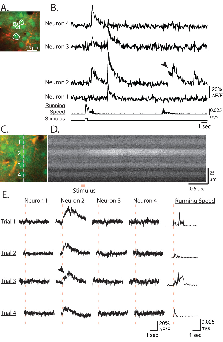
Line-scan and fast transient recordings in sensory cortex of awake mice. A) Image of neurons loaded with Calcium Green-AM (green channel) and astrocytes with SR101 (red channel). B) Fluorescence traces of the neurons shown in A from a time series recorded at 64ms/frame. C) Image of neurons loaded with Calcium Green-AM (green channel) and astrocytes with SR101 (red channel). The gray line represents the line-scanning position. D) Intensity versus time line-scan image (Trial 1) of the Calcium Green channel from the position shown in C during which an air puff stimulus was applied to the mouse. E) 4 trials of line-scan recorded fluorescence traces for the 4 neurons labeled in C. Traces are aligned to the stimulus timing (red dashed line). Mouse running speed is shown in the last column. Motion correction was not applied to the line scan recordings. Note the fast increases at the onset and the slower exponential offset decay of the fluorescence transients in all traces as well as the summation of transients in B) neuron 2 and E) neuron 2, trial 3 (arrowheads).

One possible concern when examining cell activity dependent fluorescence traces in awake behaving animals is brain motion induced fluorescence changes giving false signatures for cell activity. Even after in plane motion correction, motion causing cells to move in and out of the focal plane can still remain. To evaluate the magnitude of this problem in young WT mice, we used our Z-series image stacks to estimate the fluorescence change that would occur if a cell moved up or down with respect to the imaging plane. Across the population of cells used in the generation of Figure 6, the average change in fluorescence was 2 +/− 4% for a 2 µm up or down movement, which represent the typical maximal Z motion. Further confidence in this analysis can be provided by consideration of the ratio of positive to negative transients. Because the many tens to hundreds of cells are distributed randomly in the Z-direction on the scale of our ~2 µm thick focal plane (no preferred position of the soma with respect to the imaging plane), out of plane motion would be expected to cause an equal number of positive going (cells moving into the plane and increasing the signal) and negative going (cells moving out of the plane and decreasing the signal) false fluorescence transients. In fact, these effects are exactly what we observe for the brain motion induced small fluorescence transients seen in adult YFP mice: both in their size (<~5%) and in the near equal number of positive and negative going events (Supplemental Figure 3).

Figure 6.

Estimation of error rates for detecting cell activity related calcium transients. A–D) Histograms of positive (black) and negative (gray) going fluorescence transients of varying durations and amplitudes (in units of baseline σ). E) Quantification of error rates for detecting cell activity obtained from the ratio of the number of negative to positive events for given event amplitudes and durations. F) Negative (gray) and positive (black) event triggered average of mouse running speed. Note the sharp increase in running speed at time 0 sec (event onset) indicating a correlation between negative going fluorescence transients and the onset of running and a causal relationship between brain motion and negative going events.

In contrast to the non-cell activity dependent fluorescence of YFP, cell activity induces a transient increase in Calcium Green fluorescence. Therefore, if a majority of the observed signals in Calcium Green labeled neurons are positive going (unipolar) then they are mostly activity dependent fluorescence transients from active cells, but any deviation from unipolarity implies the existence of motion induced fluorescence changes. This effect can be quantified by calculating the ratio of negative to positive going transients, making it possible to estimate a false positive error rate for cell activity dependent increases in fluorescence. In Figure 6, we have calculated this ratio for events of varying duration and varying S/N (n=7 mice, 26 time-series at 128×128 resolution). In general, shorter, smaller S/N events are far more error prone than longer, larger S/N signals. For example, 8000 positive and 4000 negative going fluorescence signals of 0.5 sec (2 samples) duration and amplitude 2 times the fluorescence baseline standard deviation (2σ) were detected (Figure 6A). Assuming all negative going fluorescence signals are caused by brain motion (Figure 6F) and assuming an equal number of positive and negative going motion induced fluorescence signals, one can expect an error rate of ~50% due to brain motion when observing such short and small signals (Figure 6E). However, this error rate decreases dramatically for longer and higher S/N events: 4σ amplitude, 1.5 sec duration positive signals are only ~2% error prone, i.e. for every 100 positive transients of this S/N and duration assumed to be caused by neural activity only 2 would be expected to represent a false signal due to brain motion. Using these results, we highlighted the transients in Figure 4B in red that have an error rate of <5%. Of course, brain motion is not the only source of error in our system. Other sources, such as electronics or photon shot noise, also contribute and become more apparent with lower S/N; therefore our error rate estimation provides an upper bound on the percent of signals that could be associated with brain motion; it could actually be significantly less.

Using the above definition for activity dependent fluorescence signals, we found that an average of 77+/−15% of neurons in each mouse (n=7) showed at least 1 calcium transient/minute (defined as a >3σ transient with a 5% or lower error rate (Figure 6E)), while 23% of neurons displayed less than 1 transient/minute. The mean activity rate averaged across all neurons was 2.6+/−1.0 transients/minute.

Bolus loading also allowed for the recording of calcium dynamics from astrocytes that were loaded with Calcium Green-AM and identified with their specific labeling by SR101. We observed a wide variety of astrocytic calcium dynamics ranging from waves of activity spreading from astrocyte to astrocyte to synchronized periodic “bursting” activity seen across many astrocytes in the same region. As with neurons, some astrocytic activity was correlated with running behavior. An example of this is seen in a recording (0.256 sec/frame) from layer 2/3 S1HL cortex (Figure 7). The fluorescence over time of 9 astrocytic structures (soma, processes and endfeet around capillaries) is plotted (Figure 7B) along with the neuropil signal, mouse running speed, air puff stimulus and brain motion. Long duration activity can be seen in many of the structures and some of these events are correlated with running (i.e. astrocytes 1, 2 and 3). The activity was different than that for neurons and the relationship between fluorescence and running behavior is not precise: though some events in specific structures are correlated with running, other events are not. Fluorescence versus running speed correlations (Figure 7C) revealed a strong running correlation for astrocyte 1 (C >0.5), some correlation for astrocytes 2–5 (0.5> C >0.3) and little correlation for astrocytes 6–9 (0.3>C>0). The running related activity of astrocytes from these different correlation groups can also be seen in the form of running onset triggered fluorescent averages (Figure 7D); here it is clear that the onset of running correlated astrocyte activity of many of the structures is delayed by ~1–2 seconds from the onset of running. When examined across all mice (n=7, 13+/−4 time series per mouse, 4+/−3 astrocytes per time series), 11+/−12% of astrocytes showed strong (C >0.5), 29+/−16% showed some (0.5> C >0.3), and 60+/−23% showed little (0.3> C >0) running correlated activity, while 6+/−6% of astrocytic structures showed no activity during the ~3 minutes of recording.

Figure 7.

Imaging astrocytic population activity in sensory cortex of awake behaving mice. Ai) False color projection-image of the 3 minute long time series (~250 µm deep); astrocytes and neurons were loaded with Calcium Green-AM (green channel) but SR101 labeled only astrocytes (red channel). B) Fluorescence traces for the neuropil and 9 astrocytic structures outlined in Aii obtained after the time series was motion corrected. Running speed, air puff stimulus and brain displacements are also shown. C) Correlation coefficients of astrocytic structure fluorescence versus running speed. The structures were numbered throughout this figure in descending correlation coefficient order. D) Running onset triggered average of fluorescence for 5 structures with varying amounts of running correlation.

Discussion

We have developed a technique to image neural structure and function on the cellular scale in awake-behaving mice. Our method is based on a spherical treadmill that allows mice to walk and run, with no overt signs of stress, while head restrained below the objective of an upright two-photon microscope. We designed this apparatus, the head plates, and the components of the cranial window to minimize brain motion. The motion was found to be predominantly in the focal plane with maximum displacements of ~2–5µm. The relatively modest motion between brain and microscope facilitated functional imaging using calcium indicators in awake mice. This adds a new capability to in vivo TPM of the mammalian brain.

Because of the in plane confinement of motion, residual motion artifacts could be corrected using an HMM algorithm designed specifically for laser scanning microscopy. The algorithm was most useful for quantifying brain motion and, while its use was not essential when examining calcium transients from cell bodies in large populations, it aided in stabilizing cell displacements within a region of interest in order to reduce the number of brain motion related fluorescence transients (Supplemental Figure 1).

Imaging calcium dynamics in S1HL cortex demonstrated the ability to optically monitor behaviorally correlated activity from neuronal populations. The observed activity in many neurons was consistent with the S1HL cortical region that we targeted stereotactically, though some bordering sensory cortical regions could also show similar activity. Previous studies have provided evidence that somatosensory processing in mice is dependent on behavioral state (Crochet and Petersen, 2006; Ferezou et al., 2006). We found a similar dependence of neuronal response to air-puff stimulated (presumably startled mouse state) versus non air-puff stimulated (non-startled state) running which was most evident when averaged over large populations (Supplemental Figure 2A). Although this effect could be seen in some specific neurons, it was greatly variable on a single neuron basis (Supplemental Figure 2B).

In contrast to the 16% of neurons with activity patterns showing strong correlation with running (C>0.5), we found that 53% of the neuropil regions sampled showed strong running correlation. Interestingly, the neuropil transients that we measured in awake mice were smaller in amplitude than the neuronal transients (~3% versus ~20% ΔF/F) and also many times smaller than neuropil signals previously measured in anesthetized rats (Kerr et al., 2005). While the previous work in rats found a correlation of the neuropil signal with electrocorticogram recorded up/down states, the smaller amplitude transients that we measured may be explained by the reduced elecrophysiological prominence of these up/down transitions in the awake state (Destexhe et al., 2007).

We found a relatively small silent fraction (~23%) of neurons in the awake mouse sensory cortex. It is tempting to make the assumption that all of the activity seen in the ~77% of active neurons is action potential related in order to compare to extracellular recording studies that find activity from a far smaller percentage of neurons (Buzsaki, 2004; Shoham et al., 2006). Our methods should be suitable to further explore the fraction of silent neurons in the awake brain; however, since calcium transients can also accompany non-spike related events, such a comparison will require further work. In cortical neurons of anesthetized rats simultaneous calcium dynamics imaging (under similar imaging and dye loading conditions to ours) and cell-attached recordings related calcium transient amplitude to the number of underlying spikes, with single action potential evoked transients of ~10% ΔF/F (Kerr et al., 2005). Although some uncertainties remain with respect to the correspondence between our calcium transients and spiking activity, assuming our single cell baseline noise level of ~2% (4 and 8 Hz frame rates) we conclude that single action potential induced calcium transients are likely observable under our conditions in awake mice.

It was possible to follow the activity of populations of astrocytes, as well as both neurons and astrocytes simultaneously. The calcium dynamics of astrocytes were qualitatively similar to that seen in anesthetized animals, waves or synchrony that were often correlated over hundreds of microns (Nimmerjahn et al., 2004; Wang et al., 2006). We also found behaviorally correlated astrocytic activity with a delayed onset.

Comparison to other methods

Compared to our method, the main advantage of miniature head mounted microscopes is their ability to examine brain activity in a less restricted environment with more natural stimuli and motion cues. Our head restrained approach, however, may provide advantages of accessibility, the low cost of converting existing two-photon microscopes and facilitating electrode recordings. In addition, the possibilities of artificial environments, which are required by our method, may offer greater experimental control over stimuli in certain situations.

Currently, extracellular electrodes are the most common method to record single unit neural activity in behaving rodents. Extracellular techniques provide far greater temporal resolution compared to TPM, but provide a much sparser sampling of neural activity. Though inserting large arrays of electrodes can increase the cell number and spatial information (Buzsaki, 2004), the electrodes are typically spaced hundreds of microns apart and therefore reveal little information about the network micro-circuitry. Furthermore, obtaining sub-cellular activity information is difficult with extracellular recordings; TPM, however, is well suited for this application (Helmchen et al., 1999; Svoboda et al., 1997). Lastly, TPM is capable of taking advantage of a greater array of genetic manipulations possible in the mouse by, for example, recording the activity of genetically identified cell types (Wilson et al., 2007) that are indistinguishable to electrodes.

Technical outlook and applications

Our current implementation will allow for neural population activity studies on the single cell level to take place in a variety of brain regions during simple behaviors. In order to access a wider array of behavioral paradigms common in rodent research, such as navigation, sensory and motor learning tasks, we are currently designing a virtual reality system that connects the recorded treadmill movements to changing visual, olfactory and somatosensory cues provided by devices in proximity to the mouse (Holscher et al., 2005; Kleinfeld and Griesbeck, 2005). To facilitate learning paradigms, a long term (chronic) preparation is desired to repeatedly monitor cell activity over long periods of time. Although we attempted some chronic versions of the preparation presented here, we found the results of bolus loading in these experiments to be only marginally successful, perhaps due to problems associated with repeated pressure and disturbances to the brain (Xu et al., 2007).

Dynamic stabilization devices capable of compensating for animal movements (Fee, 2000) should be applicable to TPM by actively repositioning the focal spot in response to measured brain motion. Even without such a device, the low brain motion and success of our motion correction algorithm should make imaging dendritic activity during behavior possible. The recordings from the astrocytic processes in Figure 7A,B (i.e. structure 1) shows the practicality of dendritic imaging. Dye loading through either intracellular electrode (Helmchen et al., 1999; Svoboda et al., 1997), electroporation techniques (Nagayama et al., 2007; Nevian and Helmchen, 2007) or genetic approaches (Heim et al., 2007; Tallini et al., 2006) will provide improved dendritic labeling compared to the bolus loading performed here. Although our experiments were performed with the microscope objective vertically oriented, the microscope design we employed (W. Denk, MPI, Heidelberg) has the ability to rotate the objective from the vertical. This will allow imaging from more lateral brain regions while maintaining the mouse in a normal orientation.

Exciting applications of our methodology may come in combination with next generation imaging and genetic techniques. For example, deeper brain structures can be accessed using GRIN lenses (Jung et al., 2004; Levene et al., 2004). Individual neurons can be stimulated or silenced using genetically encodable light activated channels (Boyden et al., 2005; Zhang et al., 2007) and a large number of exogenous and genetically encodable contrast agents are becoming available to record changes in intracellular sodium concentration (Rose et al., 1999), cAMP (Dunn et al., 2006), membrane potential (Dombeck et al., 2005; Kuhn et al., 2004; Siegel and Isacoff, 1997), and Ras activation (Yasuda et al., 2006). Simultaneously imaging many cells throughout a 3-dimensional volume has recently been achieved (Gobel et al., 2007) and faster recording rates should be possible (Saggau, 2006). In the future, linking single cell resolution population activity with electron microscopy scale network connectivity maps (Denk and Horstmann, 2004) could help provide an extensive understanding of the neural basis for behavior.

Materials and Methods

Spherical treadmill and microscope design

Imaging was performed with a custom upright multiphoton microscope similar in design to the movable objective microscope (MOM) (Sutter Instruments; W. Denk, personal communication). A 40x, 0.8 NA objective (Olympus) was used in all experiments. The illumination source was a Ti:Sapphire laser (Mira 900, Coherent, ~100-fs pulses at 80 MHz) and the following wavelengths and emission filters were employed: YFP: ~900 nm excitation light, 680sp (Semrock, Rochester, NY) emission filter; Calcium Green and SR101: ~890 nm excitation light, 680sp (Semrock) emission filter, 535/50 (Calcium Green) green transmission and red 18° reflection filter, 610/75 (SR101) emission filter (Chroma, Rockingham, VT). ScanImage 2.0 (Pologruto et al., 2003) was used for microscope control and image acquisition. Images were acquired at 2 ms/line with frame rates of 4 (128×128 pixels), 8 (64×64) or 16 (32×32) Hz for calcium sensitive dye imaging, or 2 (256×256) or 4 (128×128) Hz for YFP imaging. Cell fluorescence traces from line-scans (2 ms/line) were smoothed over 5 time points.

A large (8 inch diameter) Styrofoam ball (Floracraft, Ludington, MI) was levitated under the microscope objective using a thin cushion of air between the ball and a custom made casting containing air jets. The casting was formed by Epoxy (BC 7069 Epoxy, Bcc Products, Franklin, IN) lining the lower ~75% of the inside of a large 8.25 inch diameter hemispherical steel ladle (McMaster-Carr, Robbinsville, NJ). The air cushion was produced by 8 symmetrical 0.25 inch diameter holes through the casting that were pressurized with air at ~50 psi. We calculate that the tangential force produced by the mouse to stop or start ball rotation is comparable to forces needed to stop or start free running, so the inertia of the ball should provide a realistic reaction force.

Two computer mice (MX-1000, Logitech, Fremont, CA) positioned 90° apart along the ball equator recorded ball motion. Event counts (700 counts/inch) per 5 ms was computer monitored using custom software (Labview); the two orthogonal displacements from each mouse were output in real time as proportional analog voltages using a D/A converter. A stimulus to the mouse’s flank (contralateral to the imaged brain hemisphere) was supplied by a ~0.5 second, ~20 psi air pulse (Pressure System IIe, Toohey Co.) through a 1 mm diameter tube. The distance and angle of the tube with respect to the mouse provided sensory stimulation of a large portion of the animal (trunk region, limbs and tail), but was not constant from trial to trial due to the shifting position of the animal. A Digidata acquisition system (1322A, Molecular Devices, Sunnyvale, CA) and PClamp software (Clampex 8.2, Molecular Devices) was used to simultaneously record the movements of the ball, the timing of the air stimulus and the command voltage for the slow imaging galvanometer in order to synchronize the animal’s running behavior with time-series movies.

Animals, training and surgery

All experiments were performed in compliance with the Guide for the Care and Use of Laboratory Animals (http://www.nap.edu/readingroom/books/labrats/). Specific protocols were approved by the Princeton University Institutional Animal Care and Use Committee. Male B6CBAF1 (5–7 weeks, used for dye injections) or female Thy 1.2 YFP-H(~16 months, no dye injections) mice were trained in pairs through the second of three training sessions. During the first session, mice were handled, with the room lights on, by a trainer wearing gloves for ~10 minutes or until the mice routinely ran from hand to hand. The mice were then transferred to the ball and allowed to move freely for ~10 minutes with the room lights on while the handler rotated the ball to keep the mice centered near the vertex. The second training session consisted of again allowing the mice to move freely on the ball for ~10–15 minutes, again with the room lights on.

Following the first two training sessions, mice were anesthetized with isoflurane, and a ~1.75 mm radius half disk (full disk center position: −1.35 caudal, 0.5 lateral) craniotomy was made over one brain hemisphere and the skull over the remaining half of the disk was thinned slightly to allow for the needed approach angle for the injection pipettes (B6CBAF1 mice). The craniotomy was flanked by 4 screws (TX000-1-1/2 self tapping screws, Small Parts Inc., Miami Lakes, FL) tapped and glued (Loctite) into the skull. The bottom piece of the metal head plate assembly was affixed to the skull via dental acrylic molded around the screws, and Kwik-Cast (World Precision Instruments) was added around the craniotomy between the plate and the skull to ensure a water-tight seal. Care was taken to avoid any glue and acrylic contact with the dura surface. Uniform thickness Kwik-Sil (World Precision Instruments, Sarasota, FL) plugs (half of a ~3.5mm diameter disk) were molded onto #1 thickness, 5mm diameter coverslips (Warner Instruments, Hamden, CT) using a custom made mold and were cut to fit the exact dimensions of the craniotomy. After dye injection (B6CBAF1 mice), the coverslip/plug combination was inserted into the seat of the bottom piece of the head plate and held rigidly in place with the top piece.

Following surgery, the third training session began by head restraining the mice on the ball in complete darkness for ~15–20 minutes. Typically it would take 5–10 minutes for the mouse to learn to balance and then begin to walk or run. Imaging commenced no more than ~1 hour, and ended ~2–3 hours, after waking from anesthesia.

Calcium indicator dye loading

A 10 mM stock of Calcium Green-1 AM in DMSO+20% pluronic (made fresh before each experiment) was diluted 10 fold into (in mM): 150 NaCl, 2.5 KCl, 10 HEPES, ~0.04 SR101, (pH=7.4). Filled 2–4 MΩ pipettes (P-2000 puller, Sutter Instruments) were beveled (BV-10, Sutter, Novato, CA) to facilitate penetration of the dura. Pipettes were advanced (MP285, Sutter) through the craniotomy at ~30° with respect to the brain surface and dye injection (0.5–0.8 psi, ~4–5 minutes) was made at a depth of ~200 µm below the cortical surface. Injections targeting the S1HL cortical region were made within the following stereotaxic coordinate range: −0.9+/−0.4 mm caudal and 1.5+/−0.5 mm lateral to Bregma (Paxinos et al., 2001)

Z-motion estimation

Z motion was estimated by comparing each frame in a time-series (before in plane motion correction) to a Z series image stack from the same region. Z series were acquired in 1 µm steps around the plane of interest. The peak value of the 2 dimensional cross-correlation was calculated for each slice in the stack normalized by subtracting the mean and dividing by the standard deviation across each Z slice. The slice with the maximal peak correlation was taken as the Z position.

Motion correction with a Hidden Markov Model

We corrected laser scanning time series on a line by line basis using an HMM, in which the hidden states are the set of possible displacements of the sample relative to the optical axis δ_x ∈ {0,±1,±2,…±Δ}, δ_y ∈ {0,±1,±2,…±Δ} where Δ is the maximum offset considered. The HMM model has two basic components. First, from the observed data the probability that line l was produced while the sample was in a displacement state (δ_x, δ_y) was calculated; we call this ${\pi }_l^{{\delta }^x,{\delta }^y}$ below (Figure 3Diii). Second, a set of transition probabilities was defined to represent a simple model of the temporal dynamics of the displacement of the sample (Figure 3Dii); we call this $T\left({\delta }_x^{l-1},{\delta }_y^{l-1}\right)\to \left({\delta }_x^l,{\delta }_y^l\right)$ below. The most likely path through the hidden states was calculated (Figure 3Di) (Rabiner, 1989).

To motivate our derivation of π and T, it is useful to formulize how laser scanning data is acquired. Let R(x, y) be the mean pixel intensity image of the sample. If the beam is at $X_i^l,Y_i^l$, for the ith pixel (i ∈ {1,2,3,…N}) of scan line l, then a pixel is acquired $(I_i^l)$ that is $R(X_i^l,Y_i^l)$ sampled with Poisson noise. Without motion, $X_i^l=i\text{and}{Y}_i^l=l\text{mod}N$as this is the beam’s raster scanning pattern. However we seek ${\delta }_x^l,{\delta }_y^l$ that corrects for the brain motion such that $X{\text{'}}_i^l=X_i^l+{\delta }_x^l,Y{\text{'}}_i^l=Y_i^l+{\delta }_y^l$ is the actual location of the beam, approximated such that the relative displacement is the same for all pixels in the same scan line.

Using the Bayesian approach of an HMM, $({\delta }_x^l,{\delta }_y^l)$ can be estimated by maximizing the probability of a displacement given the pixels acquired in that line, a reference image, and the displacements at a previous lines.

$$\mathrm{P}({\delta }_x^l,{\delta }_y^l|I_i^l,\mathrm{R})=\mathrm{P}(I_i^l|R(X{\text{'}}_i^l,Y{\text{'}}_i^l))\mathrm{P}({\delta }_x^l,{\delta }_y^l|{\delta }_x^{l-1},{\delta }_y^{l-1})={\pi }_l^{{\delta }^x,{\delta }^y}T\left({\delta }_x^{l-1},{\delta }_y^{l-1}\right)\to \left({\delta }_x^l,{\delta }_y^l\right)$$

For the first term, the probability of acquiring a pixel value can be calculated, given a displacement pair and R as

$${\pi }_{l,i}^{{\delta }^x,{\delta }^y}=\frac{{\left(\gamma R\right)}^{\gamma I}{e}^{-\gamma R}}{\left(\gamma I\right)!}$$

where γ is a calibration factor relating pixel intensity to photon number. Ultimately we are interested in maximizing with respect to $({\delta }_x^l,{\delta }_y^l)$, and thus all terms that contain only γ and $I_i^l$ can be eliminated through normalization. Expressing P as a log probability gives

$$\text{ln}\left({\pi }_{l,i}^{{\delta }^x,{\delta }^y}\right)\propto \gamma \left(I\text{ln}(R)-R\right)$$

The log probability of a given line is thus

$$\text{ln}\left({\pi }_l^{{\delta }^x,{\delta }^y}\right)=\mathrm{\sum }_{i=0}^{N-1}\text{ln}\left({\pi }_{l,i}^{{\delta }^x,{\delta }^y}\right)$$

For the second term, as the movement of the sample should be smooth T was modeled as

$$T\left({\delta }_x^{l-1},{\delta }_y^{l-1}\right)\to \left({\delta }_x^l,{\delta }_y^l\right)=\frac{1}{2\pi {\lambda }^2}{e}^{-r/\lambda }$$

where

$$r=\sqrt{{\left({\delta }_x^l-{\delta }_x^{l-1}\right)}^2+{\left({\delta }_y^l-{\delta }_y^{l-1}\right)}^2}$$

Maximizing $\mathrm{P}({\delta }_x^l,{\delta }_y^l|I_i^l,\mathrm{R})$ is a standard problem of a HMM, solved with the Vertirbi algorithm.

γ was estimated by looking at the relationship between the mean and variance of pixel intensities $\left({\sigma }_x=\sqrt{\overline{x}/\gamma }\right)$ during periods when the mouse was resting and verified through calibration control experiments. λ was chosen through expectation maximization by calculating the most likely path, and the probability of that path for a discrete set of λ values and choosing the value that produced the overall most probable path. The maximal λ was determined to within 20%. R was estimated by finding a reference image that was the frame with the minimum mean squared difference compared with its following frame. In order to assure that all these values are defined, we only considered lines where Y_l ∈ {1+Δ…N − Δ} and portions of the lines where i ∈ {1+Δ…N − Δ}. T was chosen to be a minimal model that was peaked at no movement, yet did not overly constrict larger movements of the sample. Thus, this algorithm represents a parameter free motion correction framework for laser scanning microscopy.

All movies were split into 30 second segments for this analysis in order to minimize the effects of any slow Z shifts, dye bleaching or other slow changes to image morphology. Reference frames between 30 second segments were aligned via maximal 2 dimensional cross correlation in order to create a contiguous time-series.

The simulated motion of the beam for Figure 3Bii was created by summing, on a pixel by pixel basis, the beam position during a raster scanning pattern $({\stackrel{\rightharpoonup }{S}}_i^l=(X_i^l,Y_i^l))$ with the output of a stochastically driven time series $({\stackrel{\rightharpoonup }{\varphi }}_t)$

$$\begin{array}{l}\stackrel{\rightharpoonup }{S}{\text{'}}_i^l={\stackrel{\rightharpoonup }{S}}_i^l+{\stackrel{\rightharpoonup }{\varphi }}_t\\ {\stackrel{\rightharpoonup }{\varphi }}_{t+1}=(1-\frac{1}{\tau }){\stackrel{\rightharpoonup }{\varphi }}_t+\frac{1}{\tau }(\stackrel{\rightharpoonup }{\zeta }+{\stackrel{\rightharpoonup }{D}}_t)\end{array}$$

Here t is time expressed in pixels (t=lN+i), τ is 500 pixels, and $\stackrel{\rightharpoonup }{\zeta }$ is a normally distributed random variable with σ_x = 4 and σ_y =40, and ${\stackrel{\rightharpoonup }{D}}_i$ is a step function which transitions from (0,0) to (10,-3) at line 20 (t=2560). Poisson noise was added on a pixel by pixel basis to simulate differences expected from photon counting statistics. A larger image was used as the sample to avoid ambiguities at the edges.

The time needed to correct a time-series scales linearly with the total number of lines scanned, the number of possible X, Y offset pairs. 15 minutes were required to correct the time-series from Figure 4 (1200 frames, 128×128 pixels, 5 X offsets, 5 Y offsets, 2.16 GHz processor speed, Matlab version 7.0).

Data analysis

Analysis was performed using Origin (version 7), ImageJ (1.37v), and custom scripts written in MatLab (version 7). Data are presented as mean+/−standard deviation (σ). The ROIs (rectangular or polygonal areas) were manually defined on the time projection image of the time-series to closely approximate the outline of the structure of interest. Astrocytes were identified by uptake of SR101. Although the identification of all non-SR101 labeled cells as neurons likely holds for the majority cells, we note that this population may also contain other cell types (microglia, non-SR101 labeled astrocyes, etc.). Fractional changes in fluorescence for a given frame were calculated on a pixel by pixel basis relative to the mean. The values for pixels present in the ROI after motion correction were averaged. Slow time scale changes in the fluorescence time series were removed by examining the distribution of fluorescence in a +/−15 second interval around each sample time point and subtracting the 8% percentile value. This method reliably subtracted slow changes without significantly filtering longer events that had distinct onsets and offsets. Cell-Cell correlations (Figure 4F) were calculated as the Pearson's correlation coefficient of the fluorescence traces after baseline subtraction.

For event detection in each cell, the baseline and σ were calculated from manually selected regions of the fluorescence time series that did not contain large transients. Fluorescence transients were then identified (Figure 6) as events that started when fluorescence deviated 2σ from the corrected baseline, and ended when it returned to within 0.5σ of baseline. The event duration was defined as the time period between start and end. The amplitude of the event, in units of σ, was defined as the peak fluorescence during the event duration.

Velocity components of ball motion were calculated by separately integrating the counts received at 5 ms intervals from the orthogonal motion sensors of each computer mouse, then interpolating the integrated position using a cubic spline fit with a regular 1 ms temporal interval and differentiating the position using the backward difference method. Speed was calculated as the Euclidean norm of 3 perpendicular components of ball velocity. Acceleration of the ball was estimated by fitting the speed trace with a series of line segments of length 1.5 seconds, spaced at regular 750 ms intervals. Acceleration was taken as the slope of these segments, given at the midpoint.

References

- Arieli A, Sterkin A, Grinvald A, Aertsen A. Dynamics of ongoing activity: explanation of the large variability in evoked cortical responses. Science. 1996;273:1868–1871. doi: 10.1126/science.273.5283.1868. [DOI] [PubMed] [Google Scholar]
- Berg-Johnsen J, Langmoen IA. The effect of isoflurane on excitatory synaptic transmission in the rat hippocampus. Acta Anaesthesiol Scand. 1992;36:350–355. doi: 10.1111/j.1399-6576.1992.tb03480.x. [DOI] [PubMed] [Google Scholar]
- Boyden ES, Zhang F, Bamberg E, Nagel G, Deisseroth K. Millisecond-timescale, genetically targeted optical control of neural activity. Nat Neurosci. 2005;8:1263–1268. doi: 10.1038/nn1525. [DOI] [PubMed] [Google Scholar]
- Britt RH, Rossi GT. Quantitative analysis of methods for reducing physiological brain pulsations. J Neurosci Methods. 1982;6:219–229. doi: 10.1016/0165-0270(82)90085-1. [DOI] [PubMed] [Google Scholar]
- Buzsaki G. Large-scale recording of neuronal ensembles. Nat Neurosci. 2004;7:446–451. doi: 10.1038/nn1233. [DOI] [PubMed] [Google Scholar]
- Crochet S, Petersen CC. Correlating whisker behavior with membrane potential in barrel cortex of awake mice. Nat Neurosci. 2006;9:608–610. doi: 10.1038/nn1690. [DOI] [PubMed] [Google Scholar]
- Dahmen HJ. A Simple Apparatus to Investigate the Orientation of Walking Insects. Experientia. 1980;36:685–687. [Google Scholar]
- Denk W, Horstmann H. Serial block-face scanning electron microscopy to reconstruct three-dimensional tissue nanostructure. PLoS Biol. 2004;2:e329. doi: 10.1371/journal.pbio.0020329. [DOI] [PMC free article] [PubMed] [Google Scholar]
- Denk W, Strickler JH, Webb WW. Two-Photon Laser Scanning Fluorescence Microscopy. Science. 1990;248:73–76. doi: 10.1126/science.2321027. [DOI] [PubMed] [Google Scholar]
- Denk W, Svoboda K. Photon upmanship: why multiphoton imaging is more than a gimmick. Neuron. 1997;18:351–357. doi: 10.1016/s0896-6273(00)81237-4. [DOI] [PubMed] [Google Scholar]
- Destexhe A, Hughes SW, Rudolph M, Crunelli V. Are corticothalamic 'up' states fragments of wakefulness? Trends Neurosci. 2007 doi: 10.1016/j.tins.2007.04.006. [DOI] [PMC free article] [PubMed] [Google Scholar]
- Dombeck DA, Sacconi L, Blanchard-Desce M, Webb WW. Optical recording of fast neuronal membrane potential transients in acute mammalian brain slices by second-harmonic generation microscopy. J Neurophysiol. 2005;94:3628–3636. doi: 10.1152/jn.00416.2005. [DOI] [PubMed] [Google Scholar]
- Dunn TA, Wang CT, Colicos MA, Zaccolo M, DiPilato LM, Zhang J, Tsien RY, Feller MB. Imaging of cAMP levels and protein kinase A activity reveals that retinal waves drive oscillations in second-messenger cascades. J Neurosci. 2006;26:12807–12815. doi: 10.1523/JNEUROSCI.3238-06.2006. [DOI] [PMC free article] [PubMed] [Google Scholar]
- Fee MS. Active stabilization of electrodes for intracellular recording in awake behaving animals. Neuron. 2000;27:461–468. doi: 10.1016/s0896-6273(00)00057-x. [DOI] [PubMed] [Google Scholar]
- Feng G, Mellor RH, Bernstein M, Keller-Peck C, Nguyen QT, Wallace M, Nerbonne JM, Lichtman JW, Sanes JR. Imaging neuronal subsets in transgenic mice expressing multiple spectral variants of GFP. Neuron. 2000;28:41–51. doi: 10.1016/s0896-6273(00)00084-2. [DOI] [PubMed] [Google Scholar]
- Ferezou I, Bolea S, Petersen CC. Visualizing the cortical representation of whisker touch: voltage-sensitive dye imaging in freely moving mice. Neuron. 2006;50:617–629. doi: 10.1016/j.neuron.2006.03.043. [DOI] [PubMed] [Google Scholar]
- Flusberg BA, Jung JC, Cocker ED, Anderson EP, Schnitzer MJ. In vivo brain imaging using a portable 3.9 gram two-photon fluorescence microendoscope. Opt Lett. 2005;30:2272–2274. doi: 10.1364/ol.30.002272. [DOI] [PubMed] [Google Scholar]
- Gobel W, Kampa BM, Helmchen F. Imaging cellular network dynamics in three dimensions using fast 3D laser scanning. Nat Methods. 2007;4:73–79. doi: 10.1038/nmeth989. [DOI] [PubMed] [Google Scholar]
- Heim N, Garaschuk O, Friedrich MW, Mank M, Milos RI, Kovalchuk Y, Konnerth A, Griesbeck O. Improved calcium imaging in transgenic mice expressing a troponin C-based biosensor. Nat Methods. 2007;4:127–129. doi: 10.1038/nmeth1009. [DOI] [PubMed] [Google Scholar]
- Helmchen F, Fee MS, Tank DW, Denk W. A miniature head-mounted two-photon microscope. high-resolution brain imaging in freely moving animals. Neuron. 2001;31:903–912. doi: 10.1016/s0896-6273(01)00421-4. [DOI] [PubMed] [Google Scholar]
- Helmchen F, Svoboda K, Denk W, Tank DW. In vivo dendritic calcium dynamics in deep-layer cortical pyramidal neurons. Nat Neurosci. 1999;2:989–996. doi: 10.1038/14788. [DOI] [PubMed] [Google Scholar]
- Holscher C, Schnee A, Dahmen H, Setia L, Mallot HA. Rats are able to navigate in virtual environments. J Exp Biol. 2005;208:561–569. doi: 10.1242/jeb.01371. [DOI] [PubMed] [Google Scholar]
- Holtmaat A, Wilbrecht L, Knott GW, Welker E, Svoboda K. Experience-dependent and cell-type-specific spine growth in the neocortex. Nature. 2006;441:979–983. doi: 10.1038/nature04783. [DOI] [PubMed] [Google Scholar]
- Holtmaat AJ, Trachtenberg JT, Wilbrecht L, Shepherd GM, Zhang X, Knott GW, Svoboda K. Transient and persistent dendritic spines in the neocortex in vivo. Neuron. 2005;45:279–291. doi: 10.1016/j.neuron.2005.01.003. [DOI] [PubMed] [Google Scholar]
- Jung JC, Mehta AD, Aksay E, Stepnoski R, Schnitzer MJ. In vivo mammalian brain imaging using one- and two-photon fluorescence microendoscopy. J Neurophysiol. 2004;92:3121–3133. doi: 10.1152/jn.00234.2004. [DOI] [PMC free article] [PubMed] [Google Scholar]
- Kerr JN, Greenberg D, Helmchen F. Imaging input and output of neocortical networks in vivo. Proc Natl Acad Sci U S A. 2005;102:14063–14068. doi: 10.1073/pnas.0506029102. [DOI] [PMC free article] [PubMed] [Google Scholar]
- Khabbaz AN, Tank DW. Recording head direction cells in head fixed mice. Paper presented at: Society for Neuroscience (San Diego, Ca Program No. 667.8).2004. [Google Scholar]
- Kleinfeld D, Griesbeck O. From art to engineering? The rise of in vivo mammalian electrophysiology via genetically targeted labeling and nonlinear imaging. PLoS Biol. 2005;3:e355. doi: 10.1371/journal.pbio.0030355. [DOI] [PMC free article] [PubMed] [Google Scholar]
- Kuhn B, Fromherz P, Denk W. High sensitivity of Stark-shift voltage-sensing dyes by one- or two-photon excitation near the red spectral edge. Biophys J. 2004;87:631–639. doi: 10.1529/biophysj.104.040477. [DOI] [PMC free article] [PubMed] [Google Scholar]
- Levene MJ, Dombeck DA, Kasischke KA, Molloy RP, Webb WW. In vivo multiphoton microscopy of deep brain tissue. J Neurophysiol. 2004;91:1908–1912. doi: 10.1152/jn.01007.2003. [DOI] [PubMed] [Google Scholar]
- Major G, Tank D. Persistent neural activity: prevalence and mechanisms. Curr Opin Neurobiol. 2004;14:675–684. doi: 10.1016/j.conb.2004.10.017. [DOI] [PubMed] [Google Scholar]
- Mason AC, Oshinsky ML, Hoy RR. Hyperacute directional hearing in a microscale auditory system. Nature. 2001;410:686–690. doi: 10.1038/35070564. [DOI] [PubMed] [Google Scholar]
- Nagayama S, Zeng S, Xiong W, Fletcher ML, Masurkar AV, Davis DJ, Pieribone VA, Chen WR. In vivo simultaneous tracing and ca(2+) imaging of local neuronal circuits. Neuron. 2007;53:789–803. doi: 10.1016/j.neuron.2007.02.018. [DOI] [PMC free article] [PubMed] [Google Scholar]
- Nevian T, Helmchen F. Calcium indicator loading of neurons using single-cell electroporation. Pflugers Arch. 2007 doi: 10.1007/s00424-007-0234-2. [DOI] [PubMed] [Google Scholar]
- Nimmerjahn A, Kirchhoff F, Kerr JN, Helmchen F. Sulforhodamine 101 as a specific marker of astroglia in the neocortex in vivo. Nat Methods. 2004;1:31–37. doi: 10.1038/nmeth706. [DOI] [PubMed] [Google Scholar]
- Ohki K, Chung S, Ch'ng YH, Kara P, Reid RC. Functional imaging with cellular resolution reveals precise micro-architecture in visual cortex. Nature. 2005;433:597–603. doi: 10.1038/nature03274. [DOI] [PubMed] [Google Scholar]
- Paxinos G, Franklin KBJ, Franklin KBJ. The mouse brain in stereotaxic coordinates. San Diego: Academic Press; 2001. [Google Scholar]
- Pologruto TA, Sabatini BL, Svoboda K. ScanImage: flexible software for operating laser scanning microscopes. Biomed Eng Online. 2003;2:13. doi: 10.1186/1475-925X-2-13. [DOI] [PMC free article] [PubMed] [Google Scholar]
- Rabiner LR. A Tutorial on Hidden Markov-Models and Selected Applications in Speech Recognition; Proceedings of the Ieee; 1989. pp. 257–286. [Google Scholar]
- Rose CR, Kovalchuk Y, Eilers J, Konnerth A. Two-photon Na+ imaging in spines and fine dendrites of central neurons. Pflugers Arch. 1999;439:201–207. doi: 10.1007/s004249900123. [DOI] [PubMed] [Google Scholar]
- Saggau P. New methods and uses for fast optical scanning. Curr Opin Neurobiol. 2006;16:543–550. doi: 10.1016/j.conb.2006.08.011. [DOI] [PubMed] [Google Scholar]
- Sato TR, Gray NW, Mainen ZF, Svoboda K. The Functional Microarchitecture of the Mouse Barrel Cortex. PLoS Biol. 2007;5:e189. doi: 10.1371/journal.pbio.0050189. [DOI] [PMC free article] [PubMed] [Google Scholar]
- Shoham S, O'Connor DH, Segev R. How silent is the brain: is there a "dark matter" problem in neuroscience? J Comp Physiol A Neuroethol Sens Neural Behav Physiol. 2006;192:777–784. doi: 10.1007/s00359-006-0117-6. [DOI] [PubMed] [Google Scholar]
- Siegel MS, Isacoff EY. A genetically encoded optical probe of membrane voltage. Neuron. 1997;19:735–741. doi: 10.1016/s0896-6273(00)80955-1. [DOI] [PubMed] [Google Scholar]
- Stevenson PA, Dyakonova V, Rillich J, Schildberger K. Octopamine and experience-dependent modulation of aggression in crickets. J Neurosci. 2005;25:1431–1441. doi: 10.1523/JNEUROSCI.4258-04.2005. [DOI] [PMC free article] [PubMed] [Google Scholar]
- Stosiek C, Garaschuk O, Holthoff K, Konnerth A. In vivo two-photon calcium imaging of neuronal networks. Proc Natl Acad Sci U S A. 2003;100:7319–7324. doi: 10.1073/pnas.1232232100. [DOI] [PMC free article] [PubMed] [Google Scholar]
- Svoboda K, Denk W, Kleinfeld D, Tank DW. In vivo dendritic calcium dynamics in neocortical pyramidal neurons. Nature. 1997;385:161–165. doi: 10.1038/385161a0. [DOI] [PubMed] [Google Scholar]
- Tallini YN, Ohkura M, Choi BR, Ji G, Imoto K, Doran R, Lee J, Plan P, Wilson J, Xin HB, et al. Imaging cellular signals in the heart in vivo: Cardiac expression of the high-signal Ca2+ indicator GCaMP2. Proc Natl Acad Sci U S A. 2006;103:4753–4758. doi: 10.1073/pnas.0509378103. [DOI] [PMC free article] [PubMed] [Google Scholar]
- Turner MJ, Kleeberger SR, Lightfoot JT. Influence of genetic background on daily running-wheel activity differs with aging. Physiol Genomics. 2005;22:76–85. doi: 10.1152/physiolgenomics.00243.2004. [DOI] [PubMed] [Google Scholar]
- Wang X, Lou N, Xu Q, Tian GF, Peng WG, Han X, Kang J, Takano T, Nedergaard M. Astrocytic Ca2+ signaling evoked by sensory stimulation in vivo. Nat Neurosci. 2006;9:816–823. doi: 10.1038/nn1703. [DOI] [PubMed] [Google Scholar]
- Wilson JM, Dombeck DA, Diaz-Rios M, Harris-Warrick RM, Brownstone RM. Two-Photon Calcium Imaging of Network Activity in XFP-Expressing Neurons in the Mouse. J Neurophysiol. 2007;97:3118–3125. doi: 10.1152/jn.01207.2006. [DOI] [PubMed] [Google Scholar]
- Xu HT, Pan F, Yang G, Gan WB. Choice of cranial window type for in vivo imaging affects dendritic spine turnover in the cortex. Nat Neurosci. 2007;10:549–551. doi: 10.1038/nn1883. [DOI] [PubMed] [Google Scholar]
- Yasuda R, Harvey CD, Zhong H, Sobczyk A, van Aelst L, Svoboda K. Supersensitive Ras activation in dendrites and spines revealed by two-photon fluorescence lifetime imaging. Nat Neurosci. 2006;9:283–291. doi: 10.1038/nn1635. [DOI] [PubMed] [Google Scholar]
- Zhang F, Wang LP, Brauner M, Liewald JF, Kay K, Watzke N, Wood PG, Bamberg E, Nagel G, Gottschalk A, Deisseroth K. Multimodal fast optical interrogation of neural circuitry. Nature. 2007;446:633–639. doi: 10.1038/nature05744. [DOI] [PubMed] [Google Scholar]
Associated Data
This section collects any data citations, data availability statements, or supplementary materials included in this article.