Discovering gapped binding sites of yeast transcription factors

Abstract

A gapped transcription factor-binding site (TFBS) contains one or more highly degenerate positions. Discovering gapped motifs is difficult, because allowing highly degenerate positions in a motif greatly enlarges the search space and complicates the discovery process. Here, we propose a method for discovering TFBSs, especially gapped motifs. We use ChIP-chip data to judge the binding strength of a TF to a putative target promoter and use orthologous sequences from related species to judge the degree of evolutionary conservation of a predicted TFBS. Candidate motifs are constructed by growing compact motif blocks and by concatenating two candidate blocks, allowing 0–15 degenerate positions in between. The resultant patterns are statistically evaluated for their ability to distinguish between target and nontarget genes. Then, a position-based ranking procedure is proposed to enhance the signals of true motifs by collecting position concurrences. Empirical tests on 32 known yeast TFBSs show that the method is highly accurate in identifying gapped motifs, outperforming current methods, and it also works well on ungapped motifs. Predictions on additional 54 TFs successfully discover 11 gapped and 38 ungapped motifs supported by literature. Our method achieves high sensitivity and specificity for predicting experimentally verified TFBSs.

Identification of transcription factor (TF)- binding motifs and their genomic locations is a baseline of understanding gene regulation (1, 2). A TF-binding site (TFBS) is usually 5–15 bp long and may contain a number of highly degenerate positions (known as wildcards in pattern recognition). For example, the generally accepted motifs for yeast TFs ABF1 and GAL4 are RTCAYTnnnnACG and CGGnnnnnnnnnnnCCG [supporting information (SI) Fig. 4], respectively, where “n” denotes any of the four nucleotides, i.e., a wildcard. A motif that contains one or more highly degenerate positions is called a “gapped” motif.

Many computational methods have been proposed to discover TFBSs (3–7), most of which involve the identification of overrepresented subsequences. These methods compare a set of DNA sequences that putatively contain binding sites for a particular TF with either a set of sequences that are not bound by the TF or a general background set. A search is then conducted for motifs that are overrepresented in the positive set, which should correspond to the TF-binding motif. Several algorithms, including RSAT, BioProspector, BIPAD, SeSiMCMC, SPACER, and SPACE (8–13), were especially designed for discovering gapped motifs. BioProspector allows gaps with varied lengths in a TFBS, whereas SPACE considers more than two subunits in a motif.

In recent years, various types of data in addition to genomic sequences have been used to identify TFBSs, including ChIP-chip data (14–18), microarray gene expression data (18–23), and evolutionary conservation of motif sequences (18, 24–27). These studies demonstrate that refining the list of potential target genes consistently improves the prediction accuracy of computational methods. In principle, even more powerful data mining and machine learning techniques can be developed to integrate different types of data and provide more accurate predictions of true TF-binding sites. In particular, more robust methods of finding gapped motifs may help to unravel the true regulatory structure of promoters. Toward this end, we propose a method that uses both position- and conservation-based ranking to merge information from intermediate motif patterns into gapped or ungapped motifs. Here, a position stands for a location on the promoter sequence of a potential target gene.

Central to our method is a ranking scheme that favors candidate motifs that are evolutionarily conserved, have positions that are repeatedly matched by frequently observed patterns, and are found in promoters that are bound by the TF with a high probability in ChIP-chip experiments. A segment in a promoter sequence is said to be matched by a pattern (e.g., consensus ACnCGT) if it can be aligned with the consensus without any mismatches (except wildcards), insertions, or deletions. A position in a sequence may be matched by several similar patterns. For example, the segment ACGCGT can be simultaneously matched by patterns AnGCGT, ACnCGT, ACGnGT, and so on. Our ranking scheme favors patterns that match popular positions in input sequences, positions that are matched many times by similar patterns. Instead of merging overlapped similar motifs, our method uses position concurrence as a source of signal intensity on the true binding site. The idea behind this ranking scheme is that a true motif might evolve into different forms during evolution. Note further that accounting for the TF-binding strength from ChIP-chip data has been shown to improve the reliability of inferred motifs (16). So, our method weights the contribution of each putative promoter sequence according to the probability in the ChIP-chip data that a TF binds to that promoter.

The Method

Outline of the Method.

Fig. 1 shows the flow chart of the proposed method. For TF α, ChIP-chip data are used to select a positive set (denoted by G^α) of promoter regions bound by TF α and a negative (control) set (denoted by G^−α) of unbound promoter regions (18). G^α is used in two mining steps to identify overrepresented subsequences, whereas G^−α is used to perform pattern filtering and ranking. The first mining step uses a prefix-scanning procedure for growing compact motif blocks; a compact block is a motif or part of a motif that admits at most one wildcard. Patterns that are found in G^α with a proportion larger than a predefined value (25% by default) are included in the pattern list. At the end of the first step, long enough patterns (containing at least six nonwildcards) are taken as candidate motifs. Short patterns (blocks of 3 or 4 bp) are filtered, and the remaining patterns are used in the second mining step, where each possible pair of short motif blocks are concatenated, allowing a number of successive wildcards in between the two blocks. After that, we sort the collected patterns, including the ungapped and gapped ones, based on the positions they bind, their degrees of conservation across related species, and their preferential occurrences in the promoters of the positive set relative to the negative set. Finally, patterns with high scores are merged into clusters according to their similarity in the derived position frequency matrices (PFMs).

Fig. 1.

A flow chart of the proposed method.

Growing Compact Blocks.

A compact block is a motif or part of a motif that admits at most only one wildcard. We require a motif block to have at least three nonwildcards, e.g., CGG, AnCG, or AnCGCGT. Growing motif blocks involves a procedure named bounded-prefix-growth, which takes a pattern and its projected database as inputs and tries to extend the pattern by appending one more nonwildcard to its suffix at a time. For details about the procedure of bounded-prefix-growth and the definition of projected databases, see ref. 28. The major advantage of using pattern growth (data-driven approaches) over examining all possible k-mer motifs (pattern-driven approaches) is that the search space can be effectively reduced. Another advantage is that it is not required to set the maximum length of a motif in advance. Fig. 2 provides an example with five input sequences of how a pattern tree is grown from scratch. The sequences that match the pattern are called the supporting sequences of a pattern. It is possible that a pattern matches a sequence at more than one position. Here, we define the Hit/Seq ratio of a pattern as the average number of occurrences of a pattern among its supporting sequences. As explained below in Block Filtering, Hit/Seq is helpful in screening out noisy compact blocks.

Fig. 2.

An illustration of growing a pattern tree using the bounded-prefix-growth procedure. A node in the pattern tree denotes a pattern candidate, accompanied by its complete projected database. The projected database is the collection of sequences with a match to the qualified sequence suffix pattern in the forward or reverse complement DNA sequence. The support for a pattern is defined as the ratio of distinct sequences (S1, S2, and so on), each with at least one match to the pattern over the total number of sequences in the original database. A pattern may match a sequence at more than one position. These sequences are denoted as S1.1, S1.2, and S1.3 in the projected database.

Block Filtering.

Before proceeding to the second mining step, a derived compact block is filtered out if the Hit/Seq ratio is larger than 15, a setting that was chosen from several trial runs on a validation set to be explained later (SI Table 4). A large Hit/Seq ratio implies that the compact blocks are frequently repeated in a single promoter region. Including such short repeats in the step of growing gapped motifs would result in a large number of pseudo motifs. Although these false-positive patterns can be removed by the proposed position-ranking scheme and the evolutionary conservation test, their existence greatly slows down the mining progress. In addition to the Hit/Seq ratio, we also use an upper threshold for f_−α (the proportion of sequences with a pattern P in G^−α) to eliminate repetitive elements present across different promoter sequences. A pattern is retained only if it satisfies:

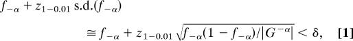where s.d. represents the standard deviation, |G^−α| is the size (number of sequences) of G^−α, z_1–0.01 is the z score at the 0.01 critical value from the standard normal distribution using the asymptotical normal approximation, and δ is set to be 0.16 on the basis of the experience in our previous study (18).

Growing Gapped Motifs.

The maximum number of consecutive wildcards between two blocks needs to be set before growing gapped motifs, the second step in the mining process. We set this value to 15. For example, CGGnnnnAnCG satisfies this criterion. Growing gapped motifs is similar to growing compact motifs, but the pattern components considered here are compact blocks, instead of a single character (nucleotide). In this study, only two blocks are used to form a pattern, although this approach could be extended to include more blocks. Although initially compact blocks with only three nonwildcards (e.g., ACC or AnCC) are considered when growing gapped motifs, true gapped motifs may contain a longer compact block on one or both ends; e.g., a gapped motif might be CCnTAnnnnnnATnGG. Such longer motif blocks are constructed by merging similar patterns hitting the same positions, as explained below in the paragraph Pattern Ranking.

Pattern Ranking.

An identified pattern is filtered out before ranking if the Hit/Seq ratio is >2, which is considered as a reasonable upper bound for selecting reliable patterns. After that, both the ungapped and gapped patterns are collected together and then ranked according to three criteria. Our first one is the preferential occurrence of a pattern in G^α relative to G^−α, denoted by S_d. Let |G^α| be the number of sequences in G^α, and |G^−α| be the number of sequences in G^−α. The proportions of sequences in G^α and G^−α that contain a pattern P are denoted as f_α and f_−α, respectively. The one-tailed two-sample proportion test can be performed as follows:

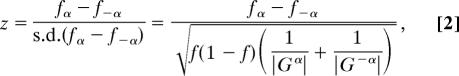where f= (|G^α|·f_α + |G^−α|·f_−α)/(|G^α| + |G^−α|). Patterns with a z score (i.e., S_d) smaller than z_1–0.01 are treated as nonsignificant and are removed before the ranking process.

The second criterion of the ranking scheme is the pattern position score, named S_p, which is derived from the popularity of positions that the pattern matches. First, a nucleotide in the promoter sequences in G^α gets one point if it is hit by a nonwildcard of a pattern. In this way, similar patterns increase their scores respectively via the number of the nucleotides they simultaneously hit. S_p is calculated by summing these nucleotide scores, normalized by the number of nonwildcard nucleotides involved. Thus, S_p is formulated as:

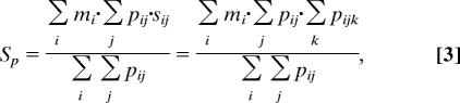where p_ij = 1 if sequence i matches the pattern and if nucleotide j of sequence i is aligned with a nonwildcard component of the pattern but p_ij = 0 if otherwise. In Eq. 3, s_ij represents the nucleotide score, defined as Σ_k p_ijk, where p_ijk = 1 if sequence i matches pattern k and if nucleotide j of sequence i is aligned with a nonwildcard component of pattern k but p_ijk = 0 if otherwise. Another term in Eq. 3 is m_i, called “sequence mask,” which is a vector of length = |G^α| and encodes the ideal matching situation in G^α. If a pattern is observed in l sequences of the positive set, the ideal situation is that it matches the top l promoter sequences with the strongest binding affinities measured by the P values in the ChIP-chip data. Therefore, we set m_i = 1 for i = 1, 2,…, l, and m_i = 0 for i = l + 1, l + 2,…, |G^α|. In other words, a pattern only accumulates its score from the frequently overlapping (popular) positions of reliable target sequences (i.e., with small P values). Further illustration of the position score and sequence mask is shown in Fig. 3. For each pattern, l is dynamically set by its support (the number of sequences it matches) in G^α. The proposed ranking scheme is similar to the idea used by the DRIM algorithm (16); however, DRIM determines a threshold to partition the input data into positive and negative samples, whereas our approach assumes that most of the input sequences are target genes of the TF of interest.

Fig. 3.

Illustration of position score accumulation and effect of sequence mask. On the promoter sequences (shown as horizontal lines), a symbol such as ▲, ■, or ● stands for a nucleotide match (a nonwildcard) in a pattern, and the numbers along with the sequences hit by motifs are nucleotide scores s_ij. In this example, motifs CCGnnnnnnCGG and AnCGnnnnnACG accumulate scores on the positions they overlap. The hit vector (A) denotes the true match pattern of a motif and the corresponding sequence mask (B) presents the ideal match pattern when the same number of matched sequences is considered. The number of “1” in the sequence mask (B) is equal to the number of matched sequences of a particular motif in G^α. The dot product of these two vectors, (A) and (B), is the final set of sequences from which the motif of interest can receive scores, which are shown in bold in (A) and (B).

The third criterion of the ranking scheme is the conservation score, S_c, which is the degree of evolutionary conservation among a set of orthologous sequences (excluding the species under study). For each pattern, the degree of conservation is assessed by the conservation of exact motif matches in S, where S is the set of orthologous sequences of genes in G^α that match the pattern. An alignment (ClustalW) of the promoter regions (500 base pairs, intergenic regions only) of the orthologues from Saccharomyces paradoxus, Saccharomyces kudriavzevii, Saccharomyces mikatae, and Saccharomyces bayanus is constructed for each gene that matches the pattern of interest. A match to an orthologue is defined as that at least one match of the motif is found within the 3 × w-bp region with respect to the hit positions in Saccharomyces cerevisiae, where w is the length of the pattern. For a gapped motif, the length includes the wildcards in between two compact blocks.

Finally, these three components are incorporated in the following equation to form the final pattern score:.

where a and b are the relative weights given to the position score and conservation score, and are empirically set to 1 and 2 (Table 1).

Table 1.

Performances of our method and some other motif finding methods in comparison to experimentally defined binding sites

TF	Our method										Other methods
	a = 1, b = 2		a = 1, b = 1		a = 0, b = 1		a = 1, b = 0		a = 0, b = 0		AlignACE		BioProspector		SPACER
	Sim.	Rank	Sim.	Rank	Sim.	Rank	Sim.	Rank	Sim.	Rank	Sim.	Rank	Sim.	Rank	Sim.	Rank
ABF1*	89.7	1	89.7	1	89.7	1	89.0	1	88.6	1	89.1	1	82.1	1	87.6	1
ACE2	90.8	1	90.8	1	90.8	1	68.6†	1	90.8	7	68.8†	4	52.0†	1	43.5†	1
BAS1	91.1	1	91.1	1	92.8	1	91.1	1	92.8	2	83.7	3	88.3	1	70.6	10
CBF1	80.6	1	79.2	1	79.2	1	84.8	1	85.5	1	81.6	1	83.9	1	81.2	1
CIN5_H2O2Lo	92.3	1	93.2	1	92.3	1	93.2	1	91.3	1	76.7	5	79.7	1	82.4	1
DIG1	93.5	1	93.5	1	93.2	1	93.5	1	93.2	3	82.4	5	89.6	1	75.7	5
FHL1*	85.2	1	85.2	1	76.5	1	82.5	1	81.9	1	88.0	1	91.3	1	88.3	1
FKH1	95.0	1	95.0	1	95.0	1	95.1	1	92.2	1	81.8	2	90.0	1	80.7	2
FKH2	91.6	1	91.6	1	91.6	1	89.8	1	89.8	1	70.8	4	88.6	1	82.8	1
GAL4_GAL*	83.3	1	83.3	1	78.1	1	70.6	1	70.8	1	78.6	1	70.0	7	81.1	1
HAP1*	72.2	1	72.2	1	72.2	1	72.2	1	72.2	1	64.0†	3	64.1†	10	76.6	7
HAP4	74.6	1	77.2	2	78.4	2	70.7	6	70.7	2	67.3†	4	76.6	5	54.0†	1
HIR1*	85.8	1	77.5	1	77.9	4	83.4	6	70.6	2	83.9	1	65.9†	8	54.9†	1
HIR2*	81.7	1	81.7	3	66.3†	10	71.0	2	68.2†	7	86.0	1	65.1†	7	86.3	1
MAC1_H2O2Hi	79.3	1	79.3	1	86.9	1	85.2	2	85.5	2	81.6	2	73.2	1	68.1†	1
MBP1	92.9	1	92.6	1	91.9	1	90.6	1	88.7	1	83.5	3	86.0	1	67.1†	3
MCM1*	79.7	1	78.0	1	78.9	1	77.0	1	77.8	1	75.1	1	76.2	1	70.9	1
MET31	71.0	1	71.0	1	70.6	2	63.8†	9	69.1†	8	71.8	4	60.7†	9	66.1†	5
MET32	76.2	3	76.6	2	72.4	3	70.3	7	70.3	10	64.3†	4	52.7†	9	57.3†	4
MET4	89.5	1	87.5	1	89.5	1	92.3	7	91.7	8	76.6	8	71.3	7	69.9†	5
MIG1	67.2†	9	68.0†	4	64.5†	4	61.9†	8	60.2†	1	67.8†	9	60.6†	3	51.5†	1
MIG2	79.3	1	79.3	2	79.3	3	79.3	2	58.6†	8	65.5†	5	54.7†	2	57.5†	8
MSN4_H2O2Hi	84.6	3	77.4	3	74.6	3	74.3	4	74.6	1	70.1	6	61.0†	8	66.3†	8
RAP1	79.6	1	74.3	1	78.8	1	73.1	1	82.4	1	83.6	1	81.6	1	80.2	1
REB1	88.7	1	88.7	1	88.7	1	88.7	1	92.8	1	90.2	1	92.2	1	92.5	1
RLM1*	87.6	1	87.6	2	87.6	6	87.6	2	67.7†	4	60.7†	3	58.2†	3	88.1	1
SMP1*	77.6	1	77.2	3	77.2	4	70.1	3	77.2	9	66.9†	10	58.1†	1	50.5†	1
STB1	81.8	1	75.8	2	79.7	1	75.8	3	71.3	1	80.1	2	74.7	1	79.2	1
STE12	86.2	1	86.6	1	86.8	1	86.4	1	87.4	1	85.3	3	85.5	1	73.0	1
SWI4	88.3	1	88.3	1	88.3	1	88.3	1	90.7	1	78.4	2	86.9	1	74.4	1
SWI5	83.3	1	83.3	1	85.4	5	85.4	4	69.8†	5	65.9†	4	52.8†	1	47.7†	1
TEC1	84.5	2	84.5	3	81.3	3	70.6	2	82.2	1	72.4	3	75.7	5	47.9†	1
Average	83.9	—	83.0		82.4		80.5		79.9		76.3		73.4		70.4
Top 1 pattern		28		22		20		16		17		9		16		14
Top 2–5 patterns		3		9		9		9		5		12		2		2
Top 6–10 patterns		0		0		1		4		4		2		2		2
The correct motif not in top 10		1		1		2		3		6		9		12		14
No. gapped motifs identified		9		9		8		9		7		6		4		7

In our method, weights a (for position score) and b (for conservation score) in Eq. 4 are set at different values. Sim., similarity of the predicted motif to the annotated PFM.

*TFs with gapped motifs.

^†Similarity scores (%)< 0.7 are considered failures.

The ranked patterns are grouped into motif clusters by an incremental clustering process. The list of ranked patterns is examined from the top, and a pattern starts to form a new cluster if it is not similar (<0.8) to any major form of the existing clusters. In each cluster, we consider the pattern with the best ranking (the highest S_pattern) as the major form and the others as the minor forms of the motif. For similarity calculation, consensuses are first transformed into PFMs based on the matched segments, and then similarity between pairs of PFMs is calculated (18, 29). The threshold 0.8 is chosen from the results of a validation set (see below). For each TF, we only consider the top 10 (top-10) motif clusters for further analysis, and for each motif cluster, four minor forms are merged with the major form to construct the final PFM. After the PFM is constructed, the scores in Eq. 4, S_d, S_p, and S_c, are adjusted accordingly to reflect the mergers of the major and minor consensus forms. In particular, the position score S_p is refined to consider only the rank property of input sequences, because the similar patterns are now merged into a single motif and their importance can be determined by the other two scores S_d and S_c. Finally, the top-10 motifs are reranked by Eq. 4 with new scores to generate the final top-10 motif list.

Performance Tests and Comparison with Other Methods

Performance Tests on Validation Data.

We first use 32 TFs with well studied motifs, collected in the MYBS database (30), as the validation set (Table 1); this set includes nine gapped motifs. For each TF, we collect a positive set of promoter sequences (G^α) with a P value <0.001 in the ChIP-chip data (29) and a negative set of promoter sequences (G^−α) with P value >0.9. The promoter sequences selected are defined as the 500-bp intergenic region upstream of the start codon ATG. For the TFs for which our method fails to recognize the correct motif as the top-1 motif when using the ChIP-chip data under the rich media condition, we investigate whether better performance can be achieved by using other available experimental conditions. If so, conditions other than rich media are used for that particular TF. There are four such TFs in the validation set: CIN5 (H2O2Lo), GAL4 (GAL), MAC1 (H2O2Hi), and MSN4 (H2O2Hi).

The mining result of our method is evaluated by looking for a motif similar to the annotated motif (listed in SI Table 5) among the top-10 patterns on the pattern list. To assess the sensitivity of our method to different parameter settings and to directly compare the performance of our method with other motif finding programs, we measure the similarity between pairs of PFMs (18, 29). When we report motif scores, a motif cluster with a better ranking is preferred as long as its match with the annotated PFM is greater than 0.7. Although scores <0.7 are considered failures, the highest similarity score found in the top-10 patterns is still reported with its rank for evaluation. The same rules are applied when examining the results of other programs.

For each of the nine gapped motifs in the validation set, the top-ranked motif identified by our method is similar (>0.77) to the annotated motif (Tables 1 and 2), except that for HAP1 the annotated gapped motif is most similar to the top-2 pattern, whereas the top-1 pattern has only the second half of the annotated motif (SI Table 5). Our predicted ungapped motifs are also consistent with the annotated PFMs (SI Table 5). Usually, the top-1 pattern has a pattern score two times larger or even higher than does the top-2 pattern, although in some cases the scores for the top two patterns are similar to each other. In SI Table 6, we show the scores of top-1 and -2 motifs, with the correct motif(s) bolded. Note that in 28 of the 32 cases, the top-1 pattern is the correct motif, although there is one case in which the top-2 pattern is also correct. In another case, the top-2 pattern is the correct motif and in other two cases the top-3 pattern is the correct motif. In only one case, our method failed to predict the correct motif within the top 10 patterns.

Table 2.

The gapped motifs found by our method vs. the annotated motifs

Note that the predicted motif of MCM1 is an ECB (a MCM1-containing complex) binding site, which has TT/AA in the flanking regions. Mcm1 binds in vivo to ECB elements throughout the cell cycle, and that binding is sensitive to carbon source changes (33).

We also evaluate the performance of our method to identify particular instances of true TFBSs from promoter sequences. We use 140 experimentally validated binding sites of 17 TFs collected from the Promoter Database of S. cerevisiae (SCPD) database (31), where 11 of the 17 TFs are from the validation set and 6 are from an additional set (see Prediction of Additional TF Motifs). For each TF, the top-1 merged PFM is used to predict binding sites. A binding-site prediction is made if the sequence of equal length to the used PFM has a similarity larger than a cutting threshold that requires ≥90% of sites matched by the consensus forms in the positive set to be predicted. A true positive requires at least a 50% overlap between the hit segment and a TF-binding site in SCPD. Table 3 reports the prediction performance. On average, the sensitivity and specificity are 69% and 74%, respectively, which suggests a favorable ability of our motifs in detecting potential binding sites when compared with the other programs investigated in (18). Note that some of the false positives predicted by the computational approaches might be true binding sites but lack experimental validation so far.

Table 3.

Accuracy of binding site prediction in comparison to annotated binding sites from the SCPD

TF	No. of sites in SCPD	Sensitivity, %	Specificity, %
ABF1	13	84.6	68.8
BAS1	9	55.6	100.0
GAL4	14	85.7	92.3
HAP1	4	50.0	50.0
HAP4	3	66.7	100.0
MAC1	5	20.0	25.0
MCM1	26	76.9	71.4
RAP1	11	100.0	64.7
REB1	12	75.0	81.8
STE12	7	71.4	71.4
SWI5	5	60.0	75.0
DAL82	2	50.0	25.0
GCN4	23	39.1	100.0
INO2	2	100.0	100.0
INO4	2	50.0	100.0
LEU3	1	100.0	50.0
UME6	1	100.0	100.0
Average		68.6	73.8

Effects of Position Scores and Conservation Scores on Performance.

Table 1 shows the results of our method on the validation set when parameters a and b in Eq. 4 are set at different values, which weight the influences of the position score and the conservation score, respectively, on the method. When a = 0 and b = 0, the patterns are selected simply according to their scores from the one-tailed two-sample proportion test. By setting a = 1, b = 0 or a = 0, b = 1, position scores or conservation score are included. Including the conservation score consistently improves the prediction of both gapped and ungapped motifs, whereas the position scoring scheme is particularly helpful for predicting gapped motifs. Several trial runs on the validation set suggest that a = 1, b = 2 performs slightly better than a = 1, b = 1 and a = 1, b = 3 (data not shown).

Comparison of Methods.

Table 1 shows a comparison of the performances of our method and three current programs, SPACER (June, 2006), AlignACE (May, 2004), and BioProspector (February, 2003) on the validation set. For the other programs, the default parameter settings are used, and for BioProspector, we do not consider gaps with varied lengths. We first compare the result of parameter setting a = 0 and b = 0 in Table 1 with the other programs. The motifs calculated by our method show an average similarity of 79.9% compared with 70.4–76.3% for the other methods. Of the 32 TFs considered, the most similar motif to the validation dataset is ranked top for 17 of our predictions, compared with only 9–14 for the other methods. By setting a = 1 and b = 2, the performance of our method is greatly improved because the similarity increased from 79.9% to 83.9%, and the correct top ranking predictions increase from 17 to 28. Thus, adding the two criteria of the score of the position matches (a = 1) and evolutionary conservation (b = 2), which are not used in the other methods compared, greatly improves the performance of our method.

Finally, we compare our study to two similar studies. The first is the DRIM (16) algorithm, which also uses a ranked list of potential target genes. In 8 of the 12 TFs found in both the predictions of DRIM and our validation set, our motifs are similar to the motifs found by DRIM (SI Table 7). For the other four TFs, our method is consistent with the literature on three TFs, whereas DRIM succeeds only on the remaining TF (MIG1). The second study is MacIsaac et al. (32), which used the improved versions of two conservation-based motif discovery algorithms, PhyloCon and Converge, to discover significant sequence motifs. The comparison is based on the 23 TFs found in both the TF list in Additional File 3 of MacIsaac et al. (32) and in our validation set; the 23 TFs include five gapped motifs. Our method discovers the correct motifs of 21 TFs, compared with the correct motifs of 20 TFs for both PhyloCon and Converge. Our method succeeds in predicting all five gapped motifs, whereas both PhyloCon and Converge succeed in predicting four gapped motifs.

Prediction of Additional TF Motifs.

We further select additional 54 TFs with experimentally annotated motifs (30), each of which has at least 15 target genes according to the ChIP-chip data (29). Eleven TFs (ARG81, ARO80, HAP3, HIR3, LEU3, NDD1, PPR1, PUT3, SIP4, STB4, and ZAP1) have been previously annotated as gapped motifs, whereas the others are ungapped motifs. Our method predicts seven gapped motifs as the top-1 pattern and the other four correct patterns are, respectively, ranked top 2 (NDD1), top 3 (PUT3), top 7 (HAP3), and top 8 (PPR1) (SI Table 8). For 30 of the 43 TFs with ungapped motifs, the top-1 pattern in our predictions is most similar to the known consensus, and eight TFs have a pattern similar to the annotated motif observed within the top-10 list.

For the five failed cases, several observations can be made. The literature-annotated motif for the NDT80-binding site is CRCAAA, but there is only one occurrence of this motif in the promoter regions of the 18 NDT80 target genes identified by the ChIP-chip experiments. This may be because NDT80 plays a central role in regulating the progression through meiosis and sporulation, whereas the available ChIP-chip experiment was conducted in rich media. Similarly, only 3 of 18 YAP3 targets contain the literature-annotated motif. Twenty-seven of 31 ADR1 target genes indeed contain occurrences of the literature defined binding motif (NGGRGK), but there are 4,566 gene promoters in the yeast genome with at least one hit for the motif. Therefore, the frequency of this motif in the positive set was not significantly higher than that in the negative set, and so it would have been discarded during the mining process. A similar problem of low-complexity motifs is found for ROX1 and for MIG1 in the validation dataset. The YAP5-binding motif provides another interesting situation: a majority of its target genes reside in the subtelomeric regions of 12 yeast chromosomes and lack orthologues in the other four species. These targets are likely duplicate genes with highly similar coding and promoter regions, making it difficult to pick out the correct motif from among these highly similar promoters.

We also applied our method to 46 TFs with unknown or crudely predicted motifs; each of these TFs has at least 15 target genes according to the ChIP-chip data (29). The results are given in SI Table 8.

Concluding Remarks

We have developed a method for discovering TFBSs, especially gapped motifs. Our method performs well when a high-quality set of potential target genes of the TF under study is available. It uses a hybrid ranking system that considers not only preferential occurrence of the motif in a set of target promoters but also the binding strength of a TF to a putative target promoter, the number of positions in the motif that are hit by similar motifs, and the degree of evolutionary conservation of a predicted TFBS. This system leads to better performance than current methods. By using a validation dataset and different weighting schemes, we determine the relevant biological criteria to accurately evaluate and compile a large number of mined candidate motifs. Compared with previous studies, the derived motifs achieve high sensitivity and specificity for predicting experimentally verified TFBSs. Our study demonstrates that hybrid data mining systems that integrate various data sources are powerful for dealing with complex biological problems.

References

- 1.Pilpel Y, Sudarsanam P, Church GM. Nat Genet. 2001;29:153–159. doi: 10.1038/ng724. [DOI] [PubMed] [Google Scholar]
- 2.Lee TI, Rinaldi NJ, Robert F, Odom DT, Bar-Joseph Z, Gerber GK, Hannett NM, Harbison CT, Thompson CM, Simon I, et al. Science. 2002;298:799–804. doi: 10.1126/science.1075090. [DOI] [PubMed] [Google Scholar]
- 3.Bulyk ML. Genome Biol. 2003;5:201. doi: 10.1186/gb-2003-5-1-201. [DOI] [PMC free article] [PubMed] [Google Scholar]
- 4.Wasserman WW, Sandelin A. Nat Rev Genet. 2004;5:276–287. doi: 10.1038/nrg1315. [DOI] [PubMed] [Google Scholar]
- 5.Hu J, Li B, Kihara D. Nucleic Acids Res. 2005;33:4899–4913. doi: 10.1093/nar/gki791. [DOI] [PMC free article] [PubMed] [Google Scholar]
- 6.Stormo GD. Bioinformatics. 2000;16:16–23. doi: 10.1093/bioinformatics/16.1.16. [DOI] [PubMed] [Google Scholar]
- 7.Tompa M, Li N, Bailey TL, Church GM, De Moor B, Eskin E, Favorov AV, Frith MC, Fu Y, Kent WJ, et al. Nat Biotechnol. 2005;23:137–144. doi: 10.1038/nbt1053. [DOI] [PubMed] [Google Scholar]
- 8.van Helden J, Rios AF, Collado-Vides J. Nucleic Acids Res. 2000;28:1808–1818. doi: 10.1093/nar/28.8.1808. [DOI] [PMC free article] [PubMed] [Google Scholar]
- 9.Liu X, Brutlag DL, Liu JS. Pac Symp Biocomput. 2001:127–138. [PubMed] [Google Scholar]
- 10.Bi C, Rogan PK. Nucleic Acids Res. 2004;32:4979–4991. doi: 10.1093/nar/gkh825. [DOI] [PMC free article] [PubMed] [Google Scholar]
- 11.Favorov AV, Gelfand MS, Gerasimova AV, Ravcheev DA, Mironov AA, Makeev VJ. Bioinformatics. 2005;21:2240–2245. doi: 10.1093/bioinformatics/bti336. [DOI] [PubMed] [Google Scholar]
- 12.Chakravarty A, Carlson JM, Khetani RS, DeZiel CE, Gross RH. Bioinformatics. 2007;23:1029–1031. doi: 10.1093/bioinformatics/btm041. [DOI] [PubMed] [Google Scholar]
- 13.Wijaya E, Rajaraman K, Yiu SM, Sung WK. Bioinformatics. 2007;23:1476–1485. doi: 10.1093/bioinformatics/btm118. [DOI] [PubMed] [Google Scholar]
- 14.Smith AD, Sumazin P, Das D, Zhang MQ. Bioinformatics 21 Suppl. 2005;1:i403–412. doi: 10.1093/bioinformatics/bti1043. [DOI] [PubMed] [Google Scholar]
- 15.Hong P, Liu XS, Zhou Q, Lu X, Liu JS, Wong WH. Bioinformatics. 2005;21:2636–2643. doi: 10.1093/bioinformatics/bti402. [DOI] [PubMed] [Google Scholar]
- 16.Eden E, Lipson D, Yogev S, Yakhini Z. PLoS Comput Biol. 2007;3:e39. doi: 10.1371/journal.pcbi.0030039. [DOI] [PMC free article] [PubMed] [Google Scholar]
- 17.Liu XS, Brutlag DL, Liu JS. Nat Biotechnol. 2002;20:835–839. doi: 10.1038/nbt717. [DOI] [PubMed] [Google Scholar]
- 18.Tsai HK, Huang GTW, Chou MY, Lu HHS, Li WH. Bioinformatics. 2006;22:1675–1681. doi: 10.1093/bioinformatics/btl160. [DOI] [PubMed] [Google Scholar]
- 19.Bannai H, Inenaga S, Shinohara A, Takeda M, Miyano S. J Bioinform Comput Biol. 2004;2:273–288. doi: 10.1142/s0219720004000612. [DOI] [PubMed] [Google Scholar]
- 20.Sinha S, Tompa M. Proc Int Conf Intell Syst Mol Biol. 2000;8:344–354. [PubMed] [Google Scholar]
- 21.Bussemaker HJ, Li H, Siggia ED. Nat Genet. 2001;27:167–171. doi: 10.1038/84792. [DOI] [PubMed] [Google Scholar]
- 22.Jensen LJ, Knudsen S. Bioinformatics. 2000;16:326–333. doi: 10.1093/bioinformatics/16.4.326. [DOI] [PubMed] [Google Scholar]
- 23.Roth FP, Hughes JD, Estep PW, Church GM. Nat Biotechnol. 1998;16:939–945. doi: 10.1038/nbt1098-939. [DOI] [PubMed] [Google Scholar]
- 24.Doniger SW, Huh J, Fay JC. Genome Res. 2005;15:701–709. doi: 10.1101/gr.3578205. [DOI] [PMC free article] [PubMed] [Google Scholar]
- 25.Elemento O, Tavazoie S. Genome Biol. 2005;6:R18. doi: 10.1186/gb-2005-6-2-r18. [DOI] [PMC free article] [PubMed] [Google Scholar]
- 26.Emberly E, Rajewsky N, Siggia ED. BMC Bioinformatics. 2003;4:57. doi: 10.1186/1471-2105-4-57. [DOI] [PMC free article] [PubMed] [Google Scholar]
- 27.Kellis M, Patterson N, Endrizzi M, Birren B, Lander ES. Nature. 2003;423:241–254. doi: 10.1038/nature01644. [DOI] [PubMed] [Google Scholar]
- 28.Hsu CM, Chen CY, Hsu CC, Liu BJ. Lecture Notes in Computer Science. 2006;3918:530–539. [Google Scholar]
- 29.Harbison CT, Gordon DB, Lee TI, Rinaldi NJ, Macisaac KD, Danford TW, Hannett NM, Tagne JB, Reynolds DB, Yoo J, et al. Nature. 2004;431:99–104. doi: 10.1038/nature02800. [DOI] [PMC free article] [PubMed] [Google Scholar]
- 30.Tsai HK, Chou MY, Shih CH, Huang GTW, Chang TH, Li WH. Nucleic Acids Res Vol. 2007;35:W221–W226. doi: 10.1093/nar/gkm379. [DOI] [PMC free article] [PubMed] [Google Scholar]
- 31.Zhu J, Zhang MQ. Bioinformatics. 1999;15:607–611. doi: 10.1093/bioinformatics/15.7.607. [DOI] [PubMed] [Google Scholar]
- 32.MacIsaac KD, Wang T, Gordon DB, Gifford DK, Stormo GD, Fraenkel E. BMC Bioinformatics. 2006;7:113. doi: 10.1186/1471-2105-7-113. [DOI] [PMC free article] [PubMed] [Google Scholar]
- 33.Mai B, Miles S, Breeden LL. Mol Cell Biol. 2002;22:430–441. doi: 10.1128/MCB.22.2.430-441.2002. [DOI] [PMC free article] [PubMed] [Google Scholar]
Associated Data
This section collects any data citations, data availability statements, or supplementary materials included in this article.