Bayesian learning of visual chunks by human observers

Abstract

Efficient and versatile processing of any hierarchically structured information requires a learning mechanism that combines lower-level features into higher-level chunks. We investigated this chunking mechanism in humans with a visual pattern-learning paradigm. We developed an ideal learner based on Bayesian model comparison that extracts and stores only those chunks of information that are minimally sufficient to encode a set of visual scenes. Our ideal Bayesian chunk learner not only reproduced the results of a large set of previous empirical findings in the domain of human pattern learning but also made a key prediction that we confirmed experimentally. In accordance with Bayesian learning but contrary to associative learning, human performance was well above chance when pair-wise statistics in the exemplars contained no relevant information. Thus, humans extract chunks from complex visual patterns by generating accurate yet economical representations and not by encoding the full correlational structure of the input.

One of the most perplexing problems facing a human learner, in domains as diverse as natural language acquisition or visual object recognition, is representing in memory the rich and hierarchically structured information present in almost every aspect of our environment (1, 2). At the core of this problem lies the task of discovering how the building blocks of a hierarchy at one level, such as words or visual chunks, are constructed from lower-level features, such as syllables or line segments (3, 4). For example, in the domain of vision, many efficient object recognition systems, both natural (5) and artificial (6), use small visual fragments (chunks) to match the parts of an image. Successful recognition of objects in these systems depends crucially on determining which parts of the image match which chunks of the prespecified inventory. However, extracting chunks from the visual input for the construction of a proper inventory entails a fundamental challenge: in any single visual scene, there are multiple objects present, often without clear segregation because of partial occlusion, clutter, and noise, and so chunks cannot be identified just by relying on low-level grouping cues. Identical arguments have been made about the challenges inherent in identifying the “chunks of language,” words, from continuous speech streams in which low-level auditory grouping cues are known to be ambiguous with respect to word boundaries (7). Therefore, to resolve the ambiguity of chunks in any single scene, or sentence, an observer needs to learn about chunks across multiple visual scenes, or sentences, and to identify chunks as consistently reappearing fragments.

Classic studies of chunking in human long-term memory revealed a variety of explicit strategies, such as verbal cue formation with highly familiar facts in a given domain (8, 9), to reduce the amount of newly stored information. However, chunking at the level of perception requires an inventory that is learned implicitly by a mechanism that is available even to infants. Within the domain of implicit chunk learning, there is substantial controversy about whether chunk learning is based on abstract rule-based operations on lower-level features or relies on associative learning of their cooccurrence statistics (10, 11). Here, we show that such implicit chunk learning cannot be explained by simple correlation-based associative learning mechanisms; rather, its characteristics can be both qualitatively and quantitatively predicted by a Bayesian chunk learner (BCL). The BCL forms chunks in a statistically principled way, without any strong prior knowledge of the possible rules for their construction, thus bridging the gap between low-level statistics and abstract rules.

Past attempts to study the learning of statistics and rules have been conducted in domains such as artificial grammar learning (12, 13), serial reaction times (14, 15), word segmentation from fluent speech (16, 17), and pattern abstraction from strings of words (18, 19). In contrast, we focus on pattern learning from multielement visual scenes (Fig. 1), because a number of subtle structural manipulations that could tease apart competing models of implicit learning have recently been conducted with such stimuli using a well controlled paradigm (20–22). We exploit this paradigm by fitting past data to the BCL and then generating a key prediction from the BCL that we test empirically in a study of human performance.

Fig. 1.

Experimental design. Schematic of scene generation in the experiments. Shapes from the inventory (Left) were organized into combos (pairs in this example). The spatial arrangement of the shapes within each combo was fixed across all scenes. For each familiarization scene, combos were pseudorandomly selected from this inventory and placed in adjacent positions within a rectangular grid (Center). Scenes were presented once every 2 sec during familiarization. The test phase consisted of 2AFC trials in which each of two scenes (Right) depicted a subset of shapes from the familiarization scenes. One subset was a true combo from the inventory (or a part thereof, called an embedded combo) and the other subset consisted of shapes from two different combos (a mixture combo).

In our visual pattern-learning paradigm, we used “combos,” combinations of shapes, as the building blocks of a series of multielement familiarization scenes (see Fig. 1 and Methods). Just as any single natural scene is formed by multiple objects or other coherent chunks, with the same object or chunk being present in several scenes, there were multiple combos shown in each familiarization scene, with the same combo reappearing across multiple scenes. Importantly, neither the human participants nor the BCL was provided with any strong low-level grouping cues identifying combos or any information about the underlying structural rules by which the visual scenes were constructed from these combos. Thus, this paradigm left statistical contingencies among the recurring shapes in the familiarization scenes as the only available cues reliably identifying individual chunks; learning was unsupervised and based entirely on mere observation of exemplars.

When learning must proceed without supervision, as in our experimental paradigm, a natural objective is that the learner should develop a faithful internal model of the environment (23). A model of the environment in our task can be formalized as a probability distribution over all possible sets of visual scenes, and the faithfulness of a model is expressed by the probability it assigns to the particular set of scenes shown in the familiarization phase. In the case of chunk learning, each inventory of chunks specifies a different distribution over scenes

The probability this distribution assigns to the set of familiarization scenes is called the likelihood of the inventory. Intuitively, the likelihood of an inventory quantifies how easy or difficult it is to piece together all previously attested visual scenes from its constituent chunks (see Methods).

Crucially, more complex inventories of chunks can generate a larger variety of possible scenes. However, because the probabilities that an inventory assigns to sets of scenes in Eq. 1 must sum to exactly 1.0, the probability value assigned to each possible set of scenes will be smaller on average for more complex inventories. This self-normalizing effect is known as the “automatic Occam's razor” property of Bayesian model comparison (24). Because of the automatic Occam's razor effect, if an inventory is too complex, its likelihood will be small, because it distributed most of its probability mass over too many other sets of scenes. Similarly, if the inventory is too simple, its likelihood will be small again, because it cannot account for all of the details of the familiarization scenes. The likelihood will be high only for an inventory whose complexity is “just right” for the given set of familiarization scenes. Thus, according to Bayesian model comparison, the optimal inventory is the one complex enough to capture previous visual experience sufficiently well but that does not over-fit the input data, which would prevent generalization to novel scenes.

For the construction of the BCL, we formalized the notion of a “chunk” as a hidden (or latent) variable that captures essential information about the presence and location of a number of shapes in the familiarization scenes. The BCL assumes that if a chunk is present in a scene, the probability that the shapes contained in that chunk are present in a particular spatial configuration in the scene is increased. If the chunk is absent from the scene, then each of the shapes contained within it have a fractional chance of appearing “spontaneously,” independently of the other shapes. Thus, although only the shapes themselves can be observed directly, chunks can be inferred as suspicious coincidences of particular shape configurations (25). This allows for computing the probability of familiarization scenes for any particular inventory (Eq. 1). Finally, the BCL applies Bayesian model comparison to compare the viability of different inventories and to prefer the one with optimal complexity [see Methods and supporting information (SI) Appendix, SI Text, and SI Tables 1–3, for further details].

Learning about chunks is but one way of forming a model of the environment, so we compared the BCL to four alternative computational models to rule out the possibility that participants used some simpler but less-optimal learning strategy. These alternative models embody the most often invoked mechanisms by which humans could learn about visual scenes or auditory sequences (26). The first two were sophisticated counting mechanisms, at the level of both individual shape frequencies and cooccurrence frequencies of shapes (see SI Appendix, SI Text). These models are typical of approaches that treat human learning as storing the averaged sum of episodic memory traces. The third model computes conditional probabilities (cooccurrence frequencies normalized by individual shape frequencies) of all possible shape pairs (see SI Appendix, SI Text). It is the most widely accepted account of human performance in statistical learning experiments in visual and auditory domains (16, 17, 20). The fourth model, the associative learner (AL), is a statistically optimal implementation of widely recognized associative learning mechanisms (27, 28). It uses a probabilistic mechanism, much like the BCL, but it keeps track of all pair-wise correlations between shapes without an explicit notion of chunks (see Methods). Here, we focus on the comparison between the AL and the BCL, because the first three models failed to capture one or more key patterns of human performance in our visual pattern-learning paradigm. For a comparison of all five models, see SI Appendix, SI Text, SI Table 4, and SI Fig. 4.

Results

To determine whether human performance is best described by the AL or the BCL, we compared the behavior of these models to the results of previously published experiments of chunk formation by humans (20, 22). These experiments provided some well quantified results that were inexplicable from the perspective of the three simpler learning models and thus established an appropriate test bed for assessing any viable theory of chunk formation (Fig. 2). The first set of these experiments showed that humans automatically extract the true pair combos from the familiarization scenes under various conditions, even when the cooccurrence frequencies of shapes bear no information about the identities of chunks (Fig. 2 A and B). These results confirmed that humans could, in principle, learn higher-order visual chunks as a part of their internal inventory. Both the AL and the BCL models could reproduce these results.

Fig. 2.

Summary of experimental manipulations [inventories (Top) and test types (Middle)], and discrimination performance (Bottom) of human participants (gray bars with dark shading indicating standard error of the mean, SEM). The predictions of the AL (pink squares) and the BCL (red stars) are shown for a series of experiments from refs 20 and 22 using increasingly complex inventories. (Colors were not included in the actual shapes seen by participants.) For a stringent comparison, the parameters of the AL were adjusted independently for each experiment to obtain best fits, whereas the BCL used a single parameter optimization across all experiments. (A) Inventory containing six equal-frequency pairs. Human performance was above chance on the basic test of true pairs vs. mixture pairs. (B) Inventory containing six pairs of varying frequency. Human performance was above chance on the test of true rare pairs vs. frequency-balanced mixture pairs. (C) Inventory containing four equal-frequency triplets. Human performance was above chance on the basic test of true triplets vs. mixture triplets and at chance on the test of embedded pairs vs. mixture pairs. (D) Inventory containing two quadruples and two pairs, all with equal frequency. Human performance was above chance on the basic tests of true quadruples or pairs vs. mixture quadruples or pairs, and on the test of embedded triplets vs. mixture triplets, but it was at chance on the test of embedded pairs vs. mixture pairs. Both models captured the overall pattern of human performance in all these experiments.

In a second set of experiments, combos with more than two shapes (triplets or quadruples) were used to create larger coherent structures to test how humans learn hierarchically structured information (Fig. 2 C and D). Just as with pairs, humans readily distinguished between these more extensive combos and random combinations of shapes. However, they produced disparate results when comparing smaller part combos (pairs or triplets), embedded in one of the true combos, with mixture combos of the same size (composed of shapes belonging to different true combos). They did not distinguish between pairs embedded in true triplets (Fig. 2C) or quadruples (Fig. 2D) from mixture pairs but could still distinguish triplets embedded in true quadruplets from mixture triplets (Fig. 2D). These results provided evidence that humans might selectively encode particular chunks while neglecting some others, depending on the hierarchical relation between the chunks. Earlier theoretical accounts of learning, captured by the three simpler models, could predict only identical performance on all test types in these experiments (see SI Appendix, SI Text, and SI Fig. 4). In contrast, both the BCL and the AL reproduced all of these results by predicting chance performance with embedded pairs and a general trend for larger embedded combos to be increasingly better recognized (SI Appendix, SI Text, and SI Figs. 4–6).

Taken together, these experiments could rule out the three simpler models as viable accounts of human visual learning, but they were insufficient to distinguish between the AL and the BCL. Although the BCL provided a substantially better quantitative fit to these data than the AL (BCL: r = 0.88, P < 0.0002, AL: r = 0.74, P < 0.01, across n = 12 different tests; see also SI Appendix, SI Figs. 5A and 6), there was no strong qualitative difference between them in predicting human behavior in these experiments.

To be able to make a qualitative distinction between the BCL and the AL, we capitalized on a crucial prediction that the BCL made and that stood in stark contrast with that derived from conventionally accepted theories, which assume that learning proceeds by computing pair-wise associations between elements (AL). The BCL, but not the AL, should be able to extract the constituent chunks of visual scenes even if pair-wise statistics between shapes contain no relevant information about chunk identity. To test this prediction, we designed an experiment that contained two groups of four shapes in which both the first- and second-order statistics between shapes were made identical (Fig. 3A). However, the shapes in one of the groups were always shown as triplet combos, whereas the shapes in the other group were shown individually (and occasionally all four of them were presented together). Consistent with the BCL, humans successfully learned to distinguish between triplets constructed from the elements of the two groups, whereas the AL was not able to make this distinction (Fig. 3B; see also SI Appendix, SI Figs. 5 and 6). Specifically, although both the BCL and the AL recognized triplets from the first group of four against mixture triplets (Fig. 3B Left), the AL, but not the BCL, also falsely recognized triplets from the second group of four (Fig. 3B Center), and the BCL but not the AL distinguished between triplets from the two groups in a direct comparison (Fig. 3B Right). This double dissociation between the BCL and the AL was also reflected in their ability to predict human performance levels in the last experiment after fitting them to all previous data (BCL: r = 0.92, P < 0.006; AL: r = −0.23, P > 0.65, across the n = 4 new test conditions; see also SI Appendix, SI Figs. 5A and 6). Thus, not only does the BCL capture human performance qualitatively better than the AL, but also it does so with a parameter-free fit of the empirical data from our final experiment.

Fig. 3.

Correlation-balanced experiment contrasting the BCL and the AL. (A) The inventory of shapes and their rules of combination. The inventory consisted of two groups of four shapes (shaded boxes), and two pairs. Shapes in the first group of 4 were always shown as one of four triplets sharing the same four shapes; shapes in the other group of 4 were shown either as single shapes or sometimes as a quadruple. The numbers below each subset of combos indicates their ratio of presentation across the entire familiarization phase. Shapes in the two groups of 4 had the same occurrence frequencies (1/2) and within-group correlations (1/3). The familiarization scenes were composed and presented the same way as in all prior experiments. (B) The three tests used to assess human performance and the actual performance (gray bars with error bars indicating SEM) along with predictions of the AL (pink bars) and the BCL (red bars). One test contrasted true triplets from the first group of 4 with mixture triplets: human performance was above chance (P < 0.017) and was predicted by both models (Left). The second test contrasted triplets constructed from the shapes of the second group of 4 (“false” triplets) with mixture triplets: human performance was not above chance (P > 0.24), and only the BCL predicted this result (Center). The final test contrasted true with false triplets: human performance was above chance (P < 0.0001), and again only the BCL predicted this result (Right). Significance was assessed by two-tailed Student's t tests.

Discussion

The present series of computational analyses and empirical findings extend previous Bayesian ideal observer analyses (29, 30) that have provided valuable insights into sensory and perceptual processing, to the domain of learning at the level of perception. Earlier work has demonstrated that humans are adapted to the environmental statistics, and they draw near-optimal perceptual inferences when faced with internal or external sources of uncertainty (31–34). However, because the learning demands of these studies were limited, the optimality of the learning process itself in such perceptual domains has not previously been addressed. Our results suggest that human chunk learning is remarkably close to optimal, especially given that participants did not become consciously aware of the existence of the combos, let alone their identities.

Our results also have implications for the distinction between statistical and rule learning. Statistical learning has been characterized as focusing on transitional or conditional probabilities that can be used to extract segments and simple chunks from the input (26) but are insufficient for learning more complex structures. In contrast, rule learning has been postulated as a qualitatively different mechanism that can capture abstract structural properties of the input that are inaccessible to any statistical learning mechanism (10, 19). Although particular details of the BCL were clearly motivated by the specific visual pattern-learning experiments we used to test our theory or by mathematical tractability, we expect its two fundamental computational principles have domain-general significance: formulating chunks as hidden variables of the environment and using Bayesian model comparison to select from alternative inventories of chunks. Thus, our results raise the possibility that, for the formation of chunks even outside the domain of vision, rule learning is merely a higher-order example of extracting hidden variables (latent structures) from a complex set of inputs in a way close to being statistically optimal. As a result, the distinction between statistical and rule learning disappears when both are considered from the perspective of Bayesian model comparison.

Bayesian model comparison, entailing the automatic Occam's razor effect, and related statistical techniques have been applied with great success to understanding various forms of learning structured information, ranging from classical conditioning in animals (35) to high-level cognitive domains in humans, such as causal induction (36), semantic representations (37), and word learning (38). Despite substantial theoretical work exploring how networks of neurons can perform at least approximate Bayes-optimal inference (39), it is still an open issue how the nervous system performs such highly complex computations efficiently in a wide variety of domains and at a number of levels of information abstraction. Establishing a formal theory of chunk learning sets the stage for subsequent algorithms that implement an ideal learner in a neurally plausible manner.

Methods

Human Experiments.

Participants were familiarized with a series of scenes composed of 12 moderately complex filled black shapes on a white background (Fig. 1). The assignment of the 12 shapes to combos was randomized across participants to control for effects due to specific shape configurations. For the construction of each scene, two or three pseudorandomly chosen combos were placed within a 3 × 3 or 5 × 5 rectangular grid. To ensure there were no obvious spatial cues identifying the combos, the positions of the combos within the grid were randomized with the constraint that at least one shape in a combo had to occupy a grid location adjacent to one shape in another combo. Across the various experiments, these constraints generated a set of 144–212 possible scenes. These scenes were presented one at a time for 2 sec, with 1-sec pauses between them, and each participant was instructed to simply view the scenes without any explicit task.

In each two-alternative forced choice (2AFC) trial of the test phase, participants were presented with two partial scenes, with the shapes approximately centered in the grid, and they selected by key press (1 or 2) the test scene more familiar based on the scenes viewed during familiarization. The two test scenes of each trial were composed according to the rules described in Fig. 2 Middle. During familiarization, participants never saw a spatially separated combo by itself, thus correct responding in the test required generalization from what had been previously seen. The order of the two test scenes in a trial was counterbalanced for each participant's test phase, and the presentation order of the test trials was individually randomized. Each test display was presented for 2 sec with a 1-sec pause between them.

Undergraduates from the University of Rochester or Brandeis University, ranging in age from 18 to 25 years, served as the participants and were paid $10 per session. There were 20–32 participants in each of the experiments. All participants were naïve with respect to the purpose of the experiment and participated only in one experiment. After the test phase was completed, participants were debriefed to determine their awareness of the underlying chunks. There was no consistent evidence in their verbal reports that the participants became aware of the underlying structure, and their confidence did not correlate with their performance in the test trials. Familiarization and test scenes were presented on a 21-in Sony Trinitron 500PS monitor at 1,024 × 728 resolution from a 1-m viewing distance. The extent of the 5 × 5 grid was 11.4°, and the maximum size of each shape was 1.14°. Stimuli were controlled by a Macintosh G4 or iMac computer by using MATLAB (Mathworks, Cambridge, U.K.) and the Psychophysics Toolbox (40). Two-tailed Student's t tests were used for assessing significance (P < 0.05) in all experiments.

All human experiments were conducted in accordance to University of Rochester or Brandeis University rules. Informed consent was obtained from all participants after the nature and possible consequences of the studies were explained. Experimental data shown in Fig. 2 and SI Appendix, SI Fig. 4 have been published (20, 22).

BCL.

The BCL represents displayed scenes with two sets of variables: observed variables corresponding to the directly observable shapes (their presence or absence encoded by binary variables y_j, and their positions encoded by 2D vectors v_j) and hidden variables, or chunks, which are revealed to the observer only indirectly through their influences on the observed shapes (their presence or absence encoded by binary variables x_i and their positions encoded by 2D vectors u_i). An inventory of chunks (I) specifies the number of hidden variables and, for each hidden variable, the observed shapes it influences. For each inventory, additional parameters (θ) quantify the magnitude of these influences (see also SI Appendix, SI Text). The task of the BCL is to infer the probability of alternative inventories after seeing the familiarization scenes.

Statistical inference requires an explicit probabilistic model of how scenes are generated. According to the generative model used by the BCL, hidden variables (chunks) appear independently from each other in each scene:

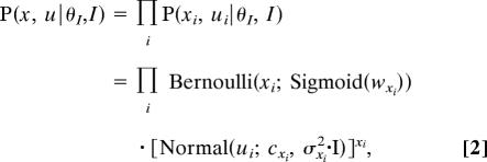where w_xi and c_xi parameterize the appearance probability x_i and preferred spatial position u_i of chunk i, and σ_xi² is its spatial variance around the preferred position, with I being the (2 × 2) identity matrix. (SI Appendix, SI Table 1 gives definitions of nonstandard function names used in equations throughout the text.)

Given a configuration of chunks, the appearances of shapes are independent:

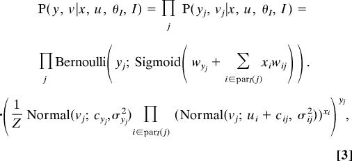where for each observed variable j, par_I(j) is the collection of hidden variables that influence it according to inventory I, matrix element w_ij quantifies the amount of influence that the presence of chunk x_i has on its presence y_j, matrix element c_ij is its preferred relative position from the center of mass of chunk u_i, w_yj and c_yj give its spontaneous appearance probability and absolute position in the absence of the chunks in par_I(j) (i.e., when its appearance is due to noise), σ_ij² and σ_yj² are the spatial variances around the respective preferred positions, and Z is an appropriate normalizing constant.

Because presented scenes specify only the appearances of the observed variables, the predictive probability of a scene is computed from Eq. 3 and by marginalizing over the values of hidden variables:

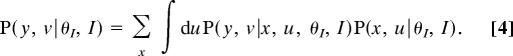Familiarization scenes, collectively constituting training data (D) for the learner, are assumed to be independent and identically distributed, thus the likelihood of an inventory with its parameters is obtained by a product of the individual predictive probabilities:

where y^(t), v^(t) are the appearances of shapes in scene t.

The marginal likelihood of an inventory (Eq. 1), which is the source of the automatic Occam's Razor effect (24), is calculated by integrating out the parameters from the parameter-dependent likelihood (Eq. 5) using a prior over parameters (see SI Appendix, SI Text and SI Table 2):

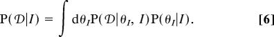According to Bayes' rule, this marginal likelihood is combined with a prior distribution over inventories (see SI Appendix, SI Text and SI Table 2) to yield a posterior distribution over inventories:

Given the posterior distribution, the predictive probability of test scene T is calculated by using again Eq. 3 and marginalizing over the posterior distribution of inventories and parameters:

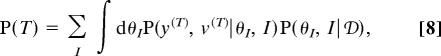where P(θ_I, I|𝒟) = P(𝒟|θ_I, I)P(θ_I|I)P(I)/P(𝒟). Because the integral implied by Eq. 8 is analytically intractable, it was approximated by a sum over samples from the joint posterior of parameters and inventories, P(θ_I, I|𝒟) (see SI Appendix, SI Text).

To provide test performances that were directly comparable to the results of the 2AFC test trials with humans, choice probability was computed as a softmax function of the log probability ratio of test scenes:

where β was the only parameter in the BCL that was used to fit simulation results to human data. (This also ensured that strictly 50% choice probability was predicted for comparisons of equally familiar scenes whose log probability ratio was zero.) It was fitted to data from Experiments 1–4 (Fig. 2), and the β value thus obtained was then used to predict experimental percent correct values (using again Eq. 9) in the correlation-balanced experiment (Fig. 3). SI Appendix, SI Fig. 5 shows the results of fitting and prediction. An earlier version of this model without a spatial component has been published (41).

AL.

The AL followed a logic very similar to that of the BCL, except that rather than assuming chunks (hidden variables) to explain dependencies between shapes, it directly learned all pair-wise statistics between them. Therefore, its task was to infer a distribution over these statistics, θ (see SI Appendix, SI Text and SI Table 3). For this, Eqs. 2–4 were substituted with the following single equation:

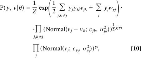where w_yj and w_jk = w_kj parameterize the occurrence and cooccurrence probabilities of shapes, just as in the Boltzmann machine (42), c_yj and c_jk = c_kj are the preferred positions and relative positions of shapes, σ_yj² and σ_jk² = σ_kj² are the spatial variances around these preferred positions, and Z is the partition function ensuring that the distribution is properly normalized.

Again, β was the only parameter that was specifically tuned to fit experimental data. For Figs. 2 and 3, parameter β (see Eq. 9) was fitted for each experiment individually, except for the baseline and frequency-balanced experiments (Fig. 2 A and B) that were fitted together (so that there were at least two data points to be fitted in each case). To facilitate a direct comparison with the capacity of the BCL for matching human performance (SI Appendix, SI Fig. 5), SI Appendix, SI Fig. 6 shows the results of fitting β with the same procedure as that used for the BCL (see also SI Appendix, SI Text).

References

- 1.Harris ZS. Structural Linguistics. Chicago: Univ of Chicago Press; 1951. [Google Scholar]
- 2.Peissig JJ, Tarr MJ. Visual object recognition: do we know more now than we did 20 years ago? Annu Rev Psychol. 2007;58:75–96. doi: 10.1146/annurev.psych.58.102904.190114. [DOI] [PubMed] [Google Scholar]
- 3.Chomsky N, Halle M. The Sound Pattern of English. Cambridge, MA: MIT Press; 1968. [Google Scholar]
- 4.Riesenhuber M, Poggio T. Hierarchical models of object recognition in cortex. Nat Neurosci. 1999;2:1019–1025. doi: 10.1038/14819. [DOI] [PubMed] [Google Scholar]
- 5.Ullman S, Vidal-Naquet M, Sali E. Visual features of intermediate complexity and their use in classification. Nat Neurosci. 2002;5:682–687. doi: 10.1038/nn870. [DOI] [PubMed] [Google Scholar]
- 6.Sudderth EB, Torralba A, Freeman WT, Willsky AS. In: Advances in Neural Information Processing Systems 18. Weiss Y, Schölkopf B, Platt J, editors. Cambridge, MA: MIT Press; 2006. pp. 1297–1304. [Google Scholar]
- 7.Christiansen MH, Allen J, Seidenberg MS. Learning to segment speech using multiple cues: a connectionist model. Lang Cognit Proc. 1998;13:221–268. [Google Scholar]
- 8.Halford GS, Cowan N, Andrews G. Separating cognitive capacity from knowledge: a new hypothesis. Trends Cognit Sci. 2007;11:236–242. doi: 10.1016/j.tics.2007.04.001. [DOI] [PMC free article] [PubMed] [Google Scholar]
- 9.Miller GA. The magical number seven plus or minus two: some limits on our capacity for processing information. Psychol Rev. 1956;63:81–97. [PubMed] [Google Scholar]
- 10.Peña M, Bonatti LL, Nespor M, Mehler J. Signal-driven computations in speech processing. Science. 2002;298:604–607. doi: 10.1126/science.1072901. [DOI] [PubMed] [Google Scholar]
- 11.Seidenberg MS, MacDonald MC, Saffran JR. Neuroscience. Does grammar start where statistics stop? Science. 2002;298:553–554. doi: 10.1126/science.1078094. [DOI] [PubMed] [Google Scholar]
- 12.Reber AS. Implicit learning of artificial grammars. J Verb Learn Verb Behav. 1967;6:855–863. [Google Scholar]
- 13.Tunney RJ, Altmann GTM. The transfer effect in artificial grammar learning: reappraising the evidence on the transfer of sequential dependencies. J Exp Psych Learn Mem Cognit. 1999;25:1322–1333. [Google Scholar]
- 14.Cleeremans A, McClelland JL. Learning the structure of event sequences. J Exp Psychol Gen. 1991;120:235–253. doi: 10.1037//0096-3445.120.3.235. [DOI] [PubMed] [Google Scholar]
- 15.Shanks DR, Johnstone T. In: Handbook of Implicit Learning. Stadler MA, French PA, editors. Thousand Oaks, CA: Sage; 1998. pp. 533–572. [Google Scholar]
- 16.Newport EL, Aslin RN. Learning at a distance I. Statistical learning of nonadjacent dependencies. Cognit Psychol. 2004;48:127–162. doi: 10.1016/s0010-0285(03)00128-2. [DOI] [PubMed] [Google Scholar]
- 17.Saffran JR, Newport EL, Aslin RN. Word Segmentation: the role of distributional cues. J Mem Lang. 1996;35:606–621. [Google Scholar]
- 18.Gomez RL, Gerken LA. Artificial grammar learning by 1-year-olds leads to specific and abstract knowledge. Cognition. 1999;70:109–135. doi: 10.1016/s0010-0277(99)00003-7. [DOI] [PubMed] [Google Scholar]
- 19.Marcus GF, Vijayan S, Bandi Rao S, Vishton PM. Rule learning by seven-month-old infants. Science. 1999;283:77–80. doi: 10.1126/science.283.5398.77. [DOI] [PubMed] [Google Scholar]
- 20.Fiser J, Aslin RN. Unsupervised statistical learning of higher-order spatial structures from visual scenes. Psychol Sci. 2001;12:499–504. doi: 10.1111/1467-9280.00392. [DOI] [PubMed] [Google Scholar]
- 21.Fiser J, Aslin RN. Statistical learning of new visual feature combinations by infants. Proc Natl Acad Sci USA. 2002;99:15822–15826. doi: 10.1073/pnas.232472899. [DOI] [PMC free article] [PubMed] [Google Scholar]
- 22.Fiser J, Aslin RN. Statistical learning of higher-order temporal structure from visual shape sequences. J Exp Psychol Gen. 2005;134:521–537. doi: 10.1037//0278-7393.28.3.458. [DOI] [PubMed] [Google Scholar]
- 23.Dayan P, Abbott LF. Theoretical Neuroscience. Cambridge, MA: MIT Press; 2001. [Google Scholar]
- 24.MacKay DJC. Information Theory, Inference, and Learning Algorithms. Cambridge, UK: Cambridge Univ Press; 2003. [Google Scholar]
- 25.Barlow HB. Unsupervised learning. Neural Comp. 1989;1:295–311. [Google Scholar]
- 26.Perruchet P, Pacton S. Implicit learning and statistical learning: one phenomenon, two approaches. Trends Cognit Sci. 2006;10:233–238. doi: 10.1016/j.tics.2006.03.006. [DOI] [PubMed] [Google Scholar]
- 27.Gallistel CR. The Organization of Learning. Cambridge, MA: Bradford Books/MIT Press; 1990. [Google Scholar]
- 28.Hebb DO. The Organization of Behavior. New York: Wiley; 1949. [Google Scholar]
- 29.Kersten D, Mamassian P, Yuille A. Object perception as Bayesian inference. Annu Rev Psychol. 2004;55:271–304. doi: 10.1146/annurev.psych.55.090902.142005. [DOI] [PubMed] [Google Scholar]
- 30.Najemnik J, Geisler WS. Optimal eye movement strategies in visual search. Nature. 2005;434:387–391. doi: 10.1038/nature03390. [DOI] [PubMed] [Google Scholar]
- 31.Stocker AA, Simoncelli EP. Noise characteristics and prior expectations in human visual speed perception. Nat Neurosci. 2006;9:578–585. doi: 10.1038/nn1669. [DOI] [PubMed] [Google Scholar]
- 32.Ernst MO, Banks MS. Humans integrate visual and haptic information in a statistically optimal fashion. Nature. 2002;415:429–433. doi: 10.1038/415429a. [DOI] [PubMed] [Google Scholar]
- 33.Körding KP, Wolpert DM. Bayesian integration in sensorimotor learning. Nature. 2004;427:244–247. doi: 10.1038/nature02169. [DOI] [PubMed] [Google Scholar]
- 34.Weiss Y, Simoncelli EP, Adelson EH. Motion illusions as optimal percepts. Nat Neurosci. 2002;5:598–604. doi: 10.1038/nn0602-858. [DOI] [PubMed] [Google Scholar]
- 35.Courville AC, Daw ND, Touretzky DS. Bayesian theories of conditioning in a changing world. Trends Cognit Sci. 2006;10:294–300. doi: 10.1016/j.tics.2006.05.004. [DOI] [PubMed] [Google Scholar]
- 36.Griffiths TL, Tenenbaum JB. Structure and strength in causal induction. Cognit Psychol. 2005;51:334–384. doi: 10.1016/j.cogpsych.2005.05.004. [DOI] [PubMed] [Google Scholar]
- 37.Griffiths TL, Steyvers M, Tenenbaum JB. Topics in semantic representation. Psychol Rev. 2007;114:211–244. doi: 10.1037/0033-295X.114.2.211. [DOI] [PubMed] [Google Scholar]
- 38.Xu F, Tenenbaum JB. Word learning as Bayesian inference. Psychol Rev. 2007;114:245–272. doi: 10.1037/0033-295X.114.2.245. [DOI] [PubMed] [Google Scholar]
- 39.Pouget A, Dayan P, Zemel R. Information processing with population codes. Nat Rev Neurosci. 2000;1:125–132. doi: 10.1038/35039062. [DOI] [PubMed] [Google Scholar]
- 40.Brainard DH. The Psychophysics Toolbox. Spatial Vision. 1997;10:433–436. [PubMed] [Google Scholar]
- 41.Orbán G, Fiser J, Aslin RN, Lengyel M. In: Advances in Neural Information Processing Systems 18. Weiss Y, Schölkopf B, Platt J, editors. Cambridge, MA: MIT Press; 2006. pp. 1043–1050. [Google Scholar]
- 42.Hinton GE, Sejnowski TJ. In: Parallel Distributed Processing: Explorations in the Microstructure of Cognition. Rumelhart DE, McClelland JL, editors. Cambridge, MA: MIT Press; 1986. [Google Scholar]
Associated Data
This section collects any data citations, data availability statements, or supplementary materials included in this article.