Abstract
Variables measured in longitudinal studies of aging and longevity do not exhaust the list of all factors affecting health and mortality transitions. Unobserved factors generate hidden variability in susceptibility to diseases and death in populations and in age trajectories of longitudinally measured indices. Effects of such heterogeneity can be manifested not only in observed hazard rates but also in average trajectories of measured indices. Although effects of hidden heterogeneity on observed mortality rates are widely discussed, their role in forming age patterns of other aging-related characteristics (average trajectories of physiological state, stress resistance, etc.) is less clear. We propose a model of hidden heterogeneity to analyze its effects in longitudinal data. The approach takes the presence of hidden heterogeneity into account and incorporates several major concepts currently developing in aging research (allostatic load, aging-associated decline in adaptive capacity and stress-resistance, age-dependent physiological norms). Simulation experiments confirm identifiability of model’s parameters.
Keywords: Aging, Longevity, Quadratic hazard model, Heterogeneity, Variability, Unobserved covariates, Longitudinal studies, Framingham Heart Study
1. Introduction
Demographic studies show that hidden differences in susceptibility to death among individuals in a population substantially affect the shapes of the mortality rates at late ages (Vaupel et al., 1979; Vaupel and Yashin, 1985). Ignoring the presence of such heterogeneity (e.g., unobserved covariates) results in underestimating regression coefficients in the Cox’s proportional hazard model. Hidden variability in other longitudinal characteristics may lead to erroneous conclusions concerning biological regularities of aging-related processes. For example, the average age trajectories of physiological indices may be biased because of effects of mortality selection. For the same reason, the evaluated decline in average resistance to stress can look slower, or become not visible. Hidden heterogeneity may also affect average trajectories of allostatic load, forces of homeostatic regulation, ‘‘optimal’’ trajectories of physiological state, magnitudes of external disturbances, etc.
Many models of hidden heterogeneity in susceptibility to death used in demography and biostatistics are identifiable. It means that distribution of unobserved heterogeneity, regression coefficients and baseline hazard can be evaluated from the data (Elbers and Ridder, 1982). Models of longitudinal data include description of dynamic properties of basic variables and their connection to mortality. Therefore, they are more complicated than mortality models traditionally used to capture unobserved heterogeneity in the populations (e.g., frailty, random effects, or latent variable models). To our knowledge, there are no results concerning conditions of identifiability in models of heterogeneity for longitudinal data. However, the presence of such heterogeneity is a realistic scenario which cannot be simply ignored in statistical analyses of longitudinal data. Our simulation studies show that parameters of the heterogeneous quadratic hazard model (QHM) are identifiable in a wide range of respective parameters values.
An important class of models for analyses of longitudinal data uses a biologically motivated assumption on a quadratic form of the hazard rates. This assumption is also supported by the evidence from epidemiological studies which found the J- or U-shapes of hazards considered as functions of risk factors (Witteman et al., 1994). These models were developed and intensively used in the studies of longitudinal data (Woodbury and Manton, 1977; Yashin, 1985; Yashin et al., 1985; Yashin and Manton, 1997; Manton and Yashin, 2000). The advantageous feature of this approach is that it allows for incorporation of the new findings and ideas appearing in the course of research on aging.
In this paper we introduce the concepts of hidden heterogeneity (discrete frailty) into the QHM. The model (referred to as ‘‘QHM with heterogeneity’’ throughout the paper) allows us to bring together, interrelate, and jointly analyze several fundamental concepts used in different studies of aging-related changes in human organisms. These include the concepts of allostatic load (Seeman et al., 2001), adaptive capacity (homeostenosis) (Troncale, 1996; Lund et al., 2002) and resistance to stresses (Semenchenko et al., 2004), as well as age-dependent physiological norms (WHO, 2000; Chobanian et al., 2003; Westin and Heath, 2005). We performed simulation studies to check the estimation procedure and performance of the model. Application of the model to the Framingham Heart Study (FHS) data on body mass index (BMI) for females illustrates the approach.
2. Model of heterogeneity in longitudinal data
Let Yt (t is age) be a continuously changing vector of random covariates (e.g., physiological indices) and Z be a hidden heterogeneity variable. It is convenient to describe evolution of Yt in the form of stochastic differential equation with coefficients depending on Z:
| (1) |
Here Wt is a Wiener process independent of the vector of initial conditions Yt0 and the random variable Z. The strength of disturbances Wt is characterized by a matrix of diffusion coefficients B (Z, t). The vector-function f1 (Z, t) (having the same dimension as a vector Yt) has a meaning of age trajectory of physiological state of the organisms subject to allostasis (McEwen and Wingfield, 2003). The organisms are forced to follow this trajectory by the process of adaptive (homeostatic) regulation. The dependence of this function on Z indicates that mechanisms of allostatic adaptation may differ for groups of individuals characterized by different values of Z. The elements of the matrix a (Z, t) correspond to the rate of adaptive response for any deviation of physiological indices Yt from f1 (Z, t) for individuals having heterogeneity variable Z.
We illustrate our approach by considering the simplest case, when the random variable Z takes two possible values “0” and “1”, P (Z = 1) = p. The extension to the case with more heterogeneity groups is straightforward. We assume that the conditional distribution of Yt0 given Z is normal with the mean m (k, t0) = mk, 0 and the variance γ(k, t0) = γk, 0, k = 0, 1. Let the mortality rate conditional on Yt and Z be a sum of a baseline (μ0) and a quadratic hazard:
| (2) |
For individuals having the heterogeneity variable Z, the baseline hazard μ0 (Z, t) characterizes the residual mortality rate, which would remain if the vector of covariates Yt follows the optimal trajectory (coinciding with the vector-function f (Z, t)). The matrix Q (Z, t) is non-negative-definite and symmetric for both values of Z and for all t from the respective interval. The vector-function f (Z, t) is introduced to explicitly characterize age-related changes in the ‘‘optimal’’ physiological state corresponding to the minimum of a hazard rate at a given age and the value of heterogeneity variable Z. It has a meaning of the age-dependent physiological norm for all individuals having the heterogeneity variable Z. It may differ from f1 (Z, t) since the process of allostatic adaptation does not necessarily result in the optimal physiological state.
Such a description corresponds to the assumption that a population under study is a mixture of two subpopulations of individuals (numbered “1” and “0”) with initial proportions p and 1 − p, respectively. These subpopulations are characterized by different dynamics of continuously changing covariates and different mortality rates. Let be a random i + 1-dimensional vector of observations of the process Yt at ages t0, t1, t2,. . ., ti, ti ≤ t < T. Denote by the conditional probability that a living individual of age t, having a sequence of measurements , belongs to the subpopulation 1. The evolution of π(t) starts at age t0 and first continues at the interval t0 ≤ t < t1; t < T. Using the Bayes formula one can show that π (t) satisfies the nonlinear differential equation (Yashin, 1985)
| (3) |
with the initial condition π(t0) = p. Here , and μ̄ (1, t) and μ̄ (0, t) are as follows:
| (4) |
where m (k, t) and γ (k, t), k = 0, 1, are the mean and the variance of the conditional distribution P (Yt ≤ y| Z = k, T > t), which satisfy the following ordinary differential equations:
| (5) |
| (6) |
at the interval t0 ≤ t < t1, with initial values m (k, t0) = mk, 0; γ (k, t0) = γk, 0, k = 0, 1. Eqs. (4)–(6) are similar to those derived in Yashin and Manton (1997) in the absence of heterogeneity.
At the age t = t1, π (t) jumps because the observation Yt1 brings new information about the value of Z. Using the Bayes rule one can easily calculate the connection between π(t1) and π(t1−) = limt↑t1 π(t):
The value π(t1) serves as an initial condition for π (t) evolving in accordance with Eq. (3) at the next age interval: t1 ≤ t < t2; t < T, and so on. Thus, π (t) evolves in accordance with (3) at the age intervals ti ≤ t < ti + 1; t < T. The initial values at the beginning of each interval are given by
respectively, m(k, t) and γ (k, t), k = 0, 1, satisfy Eqs. (5) and (6) at the intervals ti ≤ t < ti + 1, with initial values m (k, ti) = Yti; γ (k, ti) = 0, k = 0, 1. When ti ≤ t = T,
| (9) |
Thus, if we introduce where Xt = I (T ≤ t), the trajectory of π̃ (t) at the interval ti ≤ t ≤ T can be represented in terms of stochastic differential equation with one jump:
| (10) |
Here . Note that π̃ (t) I (T > t) = π (t) I (T > t). The likelihood function of the data is the product of two terms:
| (11) |
and
| (12) |
where
| (13) |
and
Here N is the number of individuals, δj is the censoring indicator (δj = 1 if jth individual died at age Tj, δj = 0 otherwise), n (j) is the number of measurements of the process Yt for jth individual. The subscript j in πj (t), yj (ti), mj (k, t), γj (k, t) indicates that respective characteristics refer to jth individual. The symbol yj (ti) denotes the value of the random process Yt measured in individual j at time ti.
3. Results
3.1. Simulation study for QHM with heterogeneity
We performed a simulation study to check performance of the model in one-dimensional case. In computer simulations, we used a discrete-time version of the model (1)–(13). We assumed that the baseline mortality in (2) is the Gompertz hazard, μ0 (k, t) = aμ0(k)ebμ0(k) (t − tmin), where tmin = 28, k = 0, 1. The quadratic hazard terms, Q (k, t), are taken as linear functions of age, Q(k, t) = aQ(k) + bQ(k) (t − tmin). To simplify calculations and to reduce the number of parameters, we assumed that the function f1 (Z, t) coincides with the optimal age trajectory of a physiological index, f (Z, t), f1 (Z, t) = f (Z, t). The optimal age-trajectories and the age-related changes in the rate of adaptive regulation are taken as linear functions, f (k, t) = af (k) + bf (k) (t − tmin) and −a (k, t) = aY (k) − bY (k) (t − tmin), where bY (k) > 0, and the strength coefficient B (k, t) is assumed to be constant, B (k, t) = σ1 (k). The initial distribution of Yt0 is normal with the mean f (k, t0) and the variance . The initial proportion of individuals in the first subpopulation (Z = 1) is denoted by p. Parameters to be estimated in this model are am0 (k), bm0 (k), aQ (k), bQ (k), af (k), bf (k), aY (k), bY (k), σ0 (k), σ1 (k), for k = 0, 1, and p. Age at entry into the study was simulated as a discrete random variable uniformly distributed over the interval [28, 62]. The interval between observations of Yt equals 2 years. The number of observations (surveys) is 25. This structure resembles the FHS data (Dawber and Kannel, 1958). Parameter values were taken close to the estimates of QHM with heterogeneity applied to the FHS data on BMI for females (see Section 3.5). We simulated 100 data sets, 2800 individuals in each data set (which is approximately equal to the number of females in the FHS data), and estimated the discrete model for different data sets using the MATLAB’s optimization toolbox (Math Works Inc., 2004).
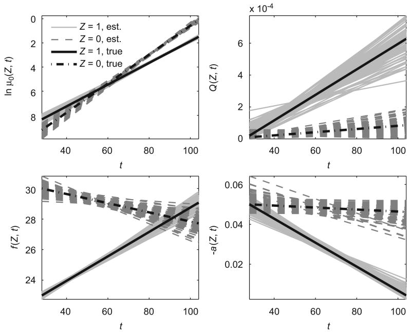
The results of this simulation study are shown in Table 1 and Fig. 1. Mean values, standard deviations and minimal and maximal values of the estimated parameters in 100 simulated data sets are presented in Table 1. Estimated trajectories of logarithms of baseline hazard, quadratic hazard terms, optimal age-trajectories of a physiological index, and age-related changes in the adaptive regulation in two subpopulations for 100 simulated data sets with hidden heterogeneity are shown in Fig. 1. Table 1 and Fig. 1 show that the estimation procedure correctly evaluates the parameters of the model and the means of all parameters are close to their true values. Thus, this procedure provides an adequate quality of estimates for a sample size comparable to that of the sex-specific FHS data and allows one to reveal hidden heterogeneity in such data.
Table 1.
Means, standard deviations (STD), minimal (MIN) and maximal (MAX) values of parameter estimates in 100 simulated data sets for QHM with heterogeneity
| aμ0 × 104 | bμ0 | aQ × 104 | bQ × 104 | aY | bY × 104 | σ0 | σ1 | af | bf | p | |
|---|---|---|---|---|---|---|---|---|---|---|---|
| Z = 1 | |||||||||||
| Mean | 2.41 | 0.090 | 0.29 | 0.077 | 0.049 | 5.81 | 3.00 | 0.90 | 22.99 | 0.080 | 0.70 |
| STD | 0.48 | 0.004 | 0.36 | 0.014 | 0.002 | 0.52 | 0.05 | 0.004 | 0.11 | 0.005 | 0.003 |
| MIN | 1.49 | 0.083 | 0.00 | 0.025 | 0.043 | 4.12 | 2.87 | 0.89 | 22.75 | 0.068 | 0.69 |
| MAX | 3.75 | 0.098 | 1.77 | 0.102 | 0.054 | 6.81 | 3.13 | 0.91 | 23.24 | 0.092 | 0.71 |
| True | 2.4 | 0.09 | 0.2 | 0.08 | 0.05 | 6.0 | 3.0 | 0.9 | 23.0 | 0.08 | 0.7 |
| Z = 0 | |||||||||||
| Mean | 0.96 | 0.121 | 0.14 | 0.009 | 0.051 | 0.75 | 5.39 | 1.60 | 29.98 | −0.029 | |
| STD | 0.29 | 0.006 | 0.16 | 0.007 | 0.003 | 0.87 | 0.14 | 0.01 | 0.31 | 0.010 | |
| MIN | 0.48 | 0.110 | 0.00 | −0.006 | 0.046 | 0.00 | 5.09 | 1.57 | 29.16 | −0.057 | |
| MAX | 1.76 | 0.134 | 0.58 | 0.024 | 0.064 | 3.57 | 5.86 | 1.63 | 30.82 | −0.006 | |
| True | 1.0 | 0.12 | 0.1 | 0.01 | 0.05 | 0.5 | 5.4 | 1.6 | 30.0 | −0.03 | |
| No Z | |||||||||||
| Mean | 2.79 | 0.092 | 0.001 | 0.032 | 0.035 | 1.07 | 4.56 | 1.15 | 25.24 | 0.040 | |
| STD | 0.41 | 0.003 | 0.007 | 0.004 | 0.002 | 0.58 | 0.07 | 0.005 | 0.13 | 0.005 | |
| MIN | 1.87 | 0.086 | 0.00 | 0.017 | 0.031 | 0.00 | 4.38 | 1.14 | 24.95 | 0.030 | |
| MAX | 4.05 | 0.099 | 0.07 | 0.043 | 0.041 | 2.73 | 4.80 | 1.16 | 25.53 | 0.049 | |
Values for QHM without heterogeneity (‘‘No Z’’) are given for comparison.
Fig. 1.
Estimated trajectories of logarithms of baseline hazard (ln μ0(Z, t)), quadratic hazard terms (Q(Z, t)), optimal values of a physiological index (f (Z, t)) and age-related changes in homeostatic capacity (−a(Z, t)) in two hypothetical subpopulations (‘‘Z = 1, est.’’ and ‘‘Z = 0, est.’’) for 100 simulated data sets with hidden heterogeneity evaluated by QHM with heterogeneity. Respective true trajectories in two subpopulations are denoted as ‘‘Z = 1, true’’ and ‘‘Z = 0, true’’.
3.2. Example: ignoring hidden heterogeneity induces inconsistency in estimates
To illustrate that ignoring hidden heterogeneity induces inconsistency in parameter estimates, we estimated simulated data sets with hidden heterogeneity (see Section 3.1) using the version of QHM without hidden heterogeneity. This model (referred to as ‘‘QHM without heterogeneity’’) is equivalent to equations (1)–(2) without dependence of Yt and μ on the heterogeneity variable Z:
| (14) |
| (15) |
where μ0(t), Q(t), f1(t), f (t), a(t), B(t), and Yt0 are equivalent to respective expressions described in the previous section but without dependence on Z. Details of the likelihood function and the estimation procedure for model Eqs. (14)–(15) can be found in Yashin et al. (2007).
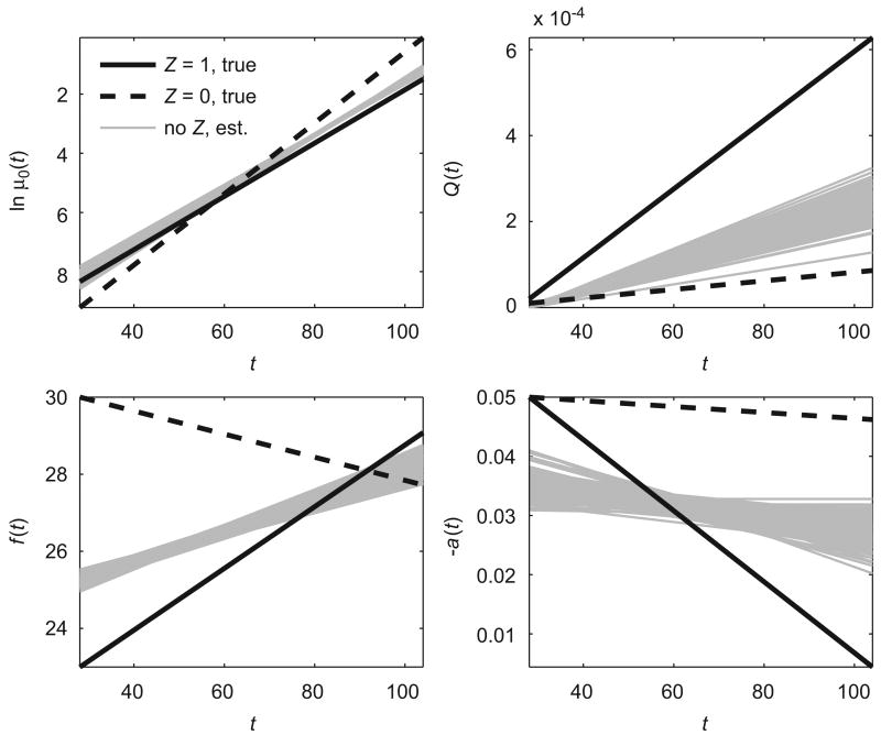
The results of this simulation study are shown in Table 1 (section ‘‘No Z’’) and Fig. 2. Table 1 illustrates that QHM without heterogeneity produces parameter estimates that deviate from respective values of parameters in two subpopulations. As a result, the population trajectories of the logarithm of the baseline hazard (ln μ0(t)), quadratic hazard terms (Q(t)), optimal age-trajectories of a physiological index (f (t)), and age-related changes in the adaptive regulation (a(t)) deviate from the true trajectories in two subpopulations (Fig. 2). Thus, ignoring hidden heterogeneity leads to incorrect estimates and wrong conclusions.
Fig. 2.
Estimated population trajectories of logarithm of baseline hazard (ln μ0(t)), quadratic hazard term (Q(t)), optimal values of a physiological index (f (t)) and age-related changes in homeostatic capacity (−a(t)) for QHM without heterogeneity (‘‘no Z, est.’’) evaluating 100 data sets simulated by QHM with heterogeneity. Respective true trajectories in two hypothetical subpopulations for QHM with heterogeneity are denoted as ‘‘Z = 1, true’’ and ‘‘Z = 0, true’’.
3.3. Example: estimates of hidden heterogeneity in data generated by a model with different structure
Simulation studies described above estimated data sets generated by QHM with heterogeneity. In real applications, however, the underlying model that generates the observed data is usually unknown. Hence, it is important to check whether the model (QHM with heterogeneity) can determine hidden heterogeneity in data generated by a model with different structure. To check this, we generated data using a model with different structure of the process Yt and mortality μ. Instead of a quadratic hazard, we used a Cox proportional hazard specification for μ:
| (16) |
In Eq. (2), we assumed a quadratic function for f1(Z, t)instead of a linear one used for QHM with heterogeneity (see Section 3.1), f1 = (Z, t) = af(Z) + bf(Z)(t − tmin) + cf(Z) (t − tmin)2 All other functions were taken equal to those described in Section 3.1.
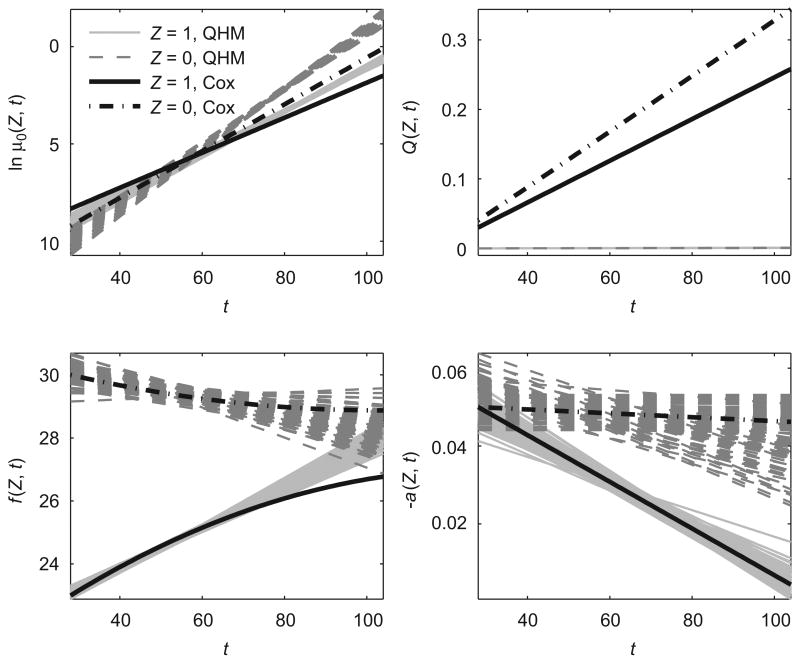
We generated 100 data sets using this model (referred to as “Cox model” throughout the text) and estimated these data sets using QHM with heterogeneity described in Section 3.1. The results are summarized in Table 2 and Fig. 3. The results indicate that, although QHM with heterogeneity fails to estimate the baseline hazard μ0(Z, t) and the function Q(Z, t) because of the difference in the structure of mortality μ in two models, it is able to determine hidden heterogeneity in data and it distinguishes trajectories of optimal values of a physiological index (f (Z, t)) and age-related changes in homeostatic capacity (−a)Z, t)) in two subpopulations. Initial proportions of individuals in these subpopulations (parameter p) are also estimated correctly.
Table 2.
Means, standard deviations (STD), minimal (MIN) and maximal (MAX) values of parameter estimates for QHM with heterogeneity evaluating 100 data sets simulated by Cox model
| aμ0 × 104 | bμ0 | aQ | bQ × 102 | aY | bY × 104 | σ0 | σ1 | af | bf | p | |
|---|---|---|---|---|---|---|---|---|---|---|---|
| Z = 1 | |||||||||||
| Mean | 1.16 | 0.111 | 0.00 | 0.001 | 0.050 | 5.90 | 3.00 | 0.90 | 23.10 | 0.064 | 0.70 |
| STD | 0.20 | 0.003 | 0.00 | 0.0001 | 0.003 | 0.61 | 0.05 | 0.004 | 0.10 | 0.004 | 0.004 |
| MIN | 0.78 | 0.102 | 0.00 | 0.0008 | 0.041 | 3.41 | 2.86 | 0.89 | 22.88 | 0.055 | 0.69 |
| MAX | 1.87 | 0.118 | 0.00 | 0.001 | 0.056 | 7.06 | 3.16 | 0.91 | 23.31 | 0.074 | 0.71 |
| True | 2.4 | 0.09 | 0.03 | 0.3 | 0.05 | 6.0 | 3.0 | 0.9 | 23.0 | 0.08 | 0.7 |
| Z = 0 | |||||||||||
| Mean | 0.49 | 0.150 | 0.00 | 0.001 | 0.052 | 1.27 | 5.39 | 1.60 | 30.02 | −0.024 | |
| STD | 0.14 | 0.006 | 0.00 | 0.0001 | 0.004 | 1.31 | 0.14 | 0.01 | 0.29 | 0.010 | |
| MIN | 0.22 | 0.135 | 0.00 | 0.001 | 0.044 | 0.00 | 5.03 | 1.58 | 29.15 | −0.048 | |
| MAX | 0.93 | 0.166 | 0.00 | 0.001 | 0.064 | 4.40 | 5.67 | 1.63 | 30.69 | 0.006 | |
| True | 1.0 | 0.12 | 0.04 | 0.4 | 0.05 | 0.5 | 5.4 | 1.6 | 30.0 | −0.03 | |
| No Z | |||||||||||
| Mean | 1.80 | 0.107 | 0.00 | 0.001 | 0.036 | 2.20 | 4.62 | 1.13 | 25.39 | 0.025 | |
| STD | 0.22 | 0.002 | 0.00 | 0.0001 | 0.003 | 0.74 | 0.06 | 0.01 | 0.12 | 0.004 | |
| MIN | 1.33 | 0.102 | 0.00 | 0.001 | 0.030 | 0.12 | 4.46 | 1.12 | 25.04 | 0.015 | |
| MAX | 2.38 | 0.113 | 0.00 | 0.001 | 0.044 | 4.40 | 4.79 | 1.15 | 25.69 | 0.037 | |
Values for QHM without heterogeneity (“No Z”) estimating these data are given for comparison.
Fig. 3.
Estimated trajectories of logarithms of baseline hazard (ln μ0(Z, t)), quadratic hazard terms (Q)Z, t)), optimal values of a physiological index (f (Z, t)) and age-related changes in homeostatic capacity (−a)Z, t)) in two hypothetical subpopulations for QHM with heterogeneity (“Z = 1, QHM” and “Z = 0, QHM”) evaluating 100 data sets simulated by Cox model. Respective true trajectories for Cox model are denoted as “Z = 1, Cox” and “Z = 0, Cox”.
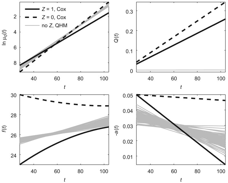
We also estimated these data using QHM without heterogeneity described in Section 3.2. The results are shown in Table 2 (section “No Z”) and Fig. 4. In this case, the population trajectories of optimal values of a physiological index (f (t)), and age-related changes in the adaptive regulation (a(t)) deviate from the true trajectories in two subpopulations (Fig. 4). Thus, the analysis of data generated by the model with different structure using the model with hidden heterogeneity improved the accuracy of calculations and conclusions.
Fig. 4.
Estimated population trajectories of logarithm of baseline hazard (ln μ0(t)), quadratic hazard term (Q(t)), optimal values of a physiological index (f (t)) and age-related changes in homeostatic capacity (−a(t)) for QHM without heterogeneity (“no Z, QHM”) evaluating 100 data sets with hidden heterogeneity simulated by Cox model. Respective true trajectories for Cox model are denoted as “Z = 1, Cox” and “Z = 0, Cox”.
3.4. Example: heterogeneity may mask the decline in stress resistance
Let us assume for simplicity that the optimal physiological state f (Z, t) does not depend on heterogeneity variable and let the conditional mortality rates for the two groups of individuals be μ(1, t, Yt) = μ1(t)(Yt −f (t))2 and μ(0, t, Yt) = μ0(t)(Yt − f (t))2. Then the mortality rate conditional on longitudinal data is
Here μ̃ (t) = μ1(t)π (t) + μ0(t)(1 − π( t)). It is clear that the rate of narrowing of the U-function of risk (which is associated with the slope of μ̃ (t)) may be lower than that in each of the two risk functions.
3.5. Application of QHM with heterogeneity to the FHS data on BMI for females
To illustrate how our approach works in applications to real data, we analyzed data on BMI for females in the FHS data using QHM with heterogeneity. The FHS cohort consists of 5209 respondents aged 28–62 years residing in Framingham, MA, between 1948 and 1952 (Dawber and Kannel, 1958). The FHS cohort is primarily white and has been followed for 50 years for the occurrence of CVD and death through surveillance of hospital admissions, death registries, and other available medical sources. Examination of participants, including an interview, a physical examination, and laboratory tests, has taken place biennially. In our analyses, we used data on BMI (which are available in all 25 exams) for 2872 females in the FHS.
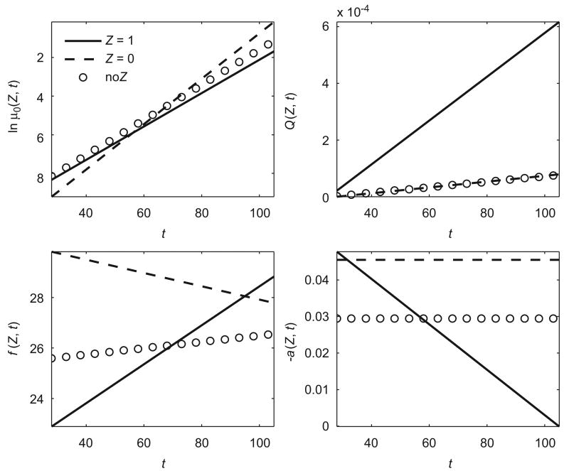
Fig. 5 illustrates the differences between mortality characteristics in two subpopulations (“Z = 1” and “Z = 0”). The first subpopulation (Z = 1) has a higher baseline mortality at younger ages and a lower baseline mortality at older ages than the second subpopulation (Z = 0) and two trajectories intersect at age about 55 years. The quadratic hazard term for the first subpopulation is higher and increases faster than that of the second subpopulation. Individuals in two subpopulations have different patterns of “optimal” trajectories of BMI (f (Z, t)), i.e., age-specific values of BMI with minimal mortality at respective ages. Individuals from the first subpopulation have an increasing pattern of “optimal” BMI starting from about 23 kg/m2 at age 28, whereas individuals from the second subpopulation have a decreasing pattern of “optimal” BMI starting from about 30 kg/m2 at age 28. Two subpopulations also have different patterns of age-related changes in the adaptive regulation (−a(Z, t)). In the first subpopulation, −a(Z, t) declines with age and in the second subpopulation it is almost constant. For comparison, Fig. 5 also shows respective population trajectories estimated by QHM without heterogeneity (“no Z”). It shows, in particular, that the population “optimal” age-trajectory of BMI deviates from the “optimal” trajectories in the subpopulations.
Fig. 5.
Estimated trajectories of logarithms of baseline hazard (ln μ0(Z, t)), quadratic hazard terms (Q(Z, t)), optimal values of a physiological index (f (Z, t)) and age-related changes in homeostatic capacity (−a(Z, t)) in two subpopulations (“Z = 1” and “Z = 0”) for QHM with heterogeneity applied to the FHS data on BMI for females. Population estimates of respective characteristics for QHM model without heterogeneity (“no Z”) are shown for comparison.
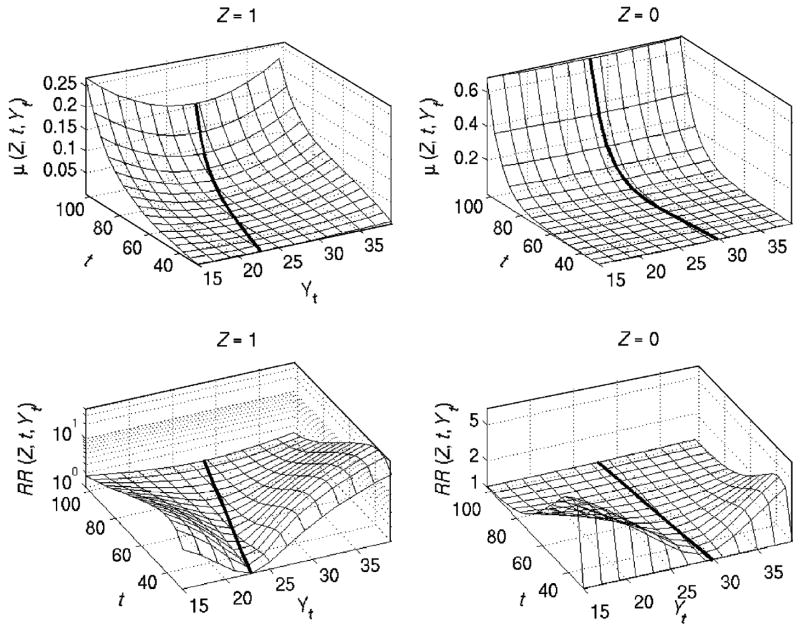
Fig. 6 displays mortality rates (μ( Z, t, Yt)) and relative risks of death (RR(Z, t, Yt)) over age (t) and values of BMI at age t (Yt) for two subpopulations. It shows that the mortality rate for the first subpopulation has a more pronounced quadratic pattern (due to higher trajectories of Q(Z, t)) and the respective U-shape of mortality risk is narrowing with age (due to the respective increase in Q(Z, t) with age). In the second subpopulation, the mortality rate does not exhibit a visible quadratic pattern. Thus, individuals from this subpopulation are less sensitive to changes in BMI with respect to mortality risks. The narrowing U-shape of risk indicates the aging-related decline in resistance to stress. This finding is in line with the results obtained in animal aging studies, which show a strong connection between the stress resistance and longevity, as well as the decline with age in resistance to many stresses (Semenchenko et al., 2004). Both subpopulations revealed similar behavior of the relative risk with increasing age. Contrary to the mortality risk, it decreases with age and manifests a widening U-shape. Such behavior may indicate the increasing role of senescence in the total mortality compared to selected risk factors in aging individuals.
Fig. 6.
Estimated mortality rates (μ( Z, t, Yt)) and relative risks of death (RR (Z, t, Yt), logarithmic scale) over age (t) and values of a physiological index at age t (Yt) in two subpopulations (“Z = 1” and “Z = 0”) for QHM with heterogeneity applied to the FHS data on BMI for females. Thick black lines denote optimal age-trajectories of BMI (f (Z, t)) in respective subpopulations.
4. Conclusions
The model proposed in this paper puts together different concepts capable of capturing fundamental features of aging-related changes including the notion of allostasis, a decline in adaptive capacity and in resistance to stresses, the aging-related physiological norms, and hidden heterogeneity in longitudinal data, and connects all these concepts to mortality (or incidence) rates. Such a model provides a possibility to develop comprehensive systemic methodology for analyses of available data on aging-related phenomena. Simulation studies showed that the estimation procedure provides an adequate quality of estimates for a moderate sample size comparable to that of the sex-specific FHS data.
Incorporation of a concept of hidden heterogeneity (discrete frailty) allows one to reveal differences in aging-related physiological parameters in individuals represented by distinct heterogeneity groups summarizing unobserved aging- and mortality-related factors (genetic and non-genetic). Individuals may differ in characteristics of allostatic load, forces of adaptive regulation, “optimal” trajectories of physiological state, magnitudes of external disturbances, etc. All such differences may be identified in the proposed model. A statistical analysis of such differences may be performed using the likelihood ratio test comparing the model with equal and non-equal trajectories in two subpopulations.
Ignoring hidden heterogeneity in aging-related characteristics may affect conclusions about regularities of respective processes. Differential selection can produce patterns of mortality or aging-related characteristics for the population as a whole that are qualitatively different from the patterns for respective subpopulations (Vaupel and Yashin, 1985). For example, if the difference between the “optimal” age-trajectories of a physiological index (f (Z, t)) in two subpopulations is ignored and the resulting observed age-trajectory in the entire population is taken as a universal “optimal” trajectory, then this “universal trajectory” will be not optimal for individuals from either of the two subpopulations. Therefore, if policy recommendations and health interventions are based on this “universal” trajectory aiming to keep an individual’s age-trajectory close to this “population” trajectory, then this will actually increase the individual’s chances of death due to increasing deviations from the true “optimal” trajectory in a respective subpopulation.
Note that although the conditional distribution of random continuously changing covariates among survivors is not Gaussian, the entire situation can be exactly described in terms of first two conditional moments of two Gaussian distributions and the conditional proportion of individuals in respective groups. The result can be easily extended to include more heterogeneity groups comprising the entire population. Another possible extension of the model is to include a concept of changing frailty. That is, instead of a frailty variable Z (which is fixed for the entire life span of an individual) one can use a hidden jumping process Zt representing changes in a (discrete) hidden heterogeneity state over time. Such a model can be useful in analyses of longitudinal data where health histories are unobserved or only partly observed. The estimation methods for such types of quadratic hazard models driven by a non-Markovian stochastic process need to be developed and validated in simulation studies for subsequent use in analyses of longitudinal data.
Acknowledgments
The Framingham Heart Study (FHS) is conducted and supported by the NHLBI in collaboration with the FHS Investigators. This manuscript was prepared using a limited access dataset obtained by the NHLBI and does not necessarily reflect the opinions or views of the FHS or the NHLBI. The work on this manuscript was supported by the NIH/NIA Grants 1R01 AG028259-01, 1RO1-AG-027019-01 and 5PO1-AG-008761-16.
References
- Chobanian AV, Bakris GL, Black HR, Cushman WC, Green LA, Izzo JL, Jr, Jones DW, Materson BJ, Oparil S, Wright JT, Jr, Roccella EJ. Joint National Committee on Prevention, Detection, Evaluation, and Treatment of High Blood Pressure. National Heart, Lung, and Blood Institute; National High Blood Pressure Education Program Coordinating Committee Seventh report of the Joint National Committee on Prevention, Detection, Evaluation, and Treatment of High Blood Pressure Hypertension. 2003;42(6):1206–1252. doi: 10.1161/01.HYP.0000107251.49515.c2. [DOI] [PubMed] [Google Scholar]
- Dawber TR, Kannel WB. An epidemiologic study of heart disease: the Framingham Study. Nutr Rev. 1958;16:1–4. doi: 10.1111/j.1753-4887.1958.tb00605.x. [DOI] [PubMed] [Google Scholar]
- Elbers C, Ridder G. True and spurious duration dependence: the identifiability of the proportional hazards model. Rev Econ Stud. 1982;49:403–409. [Google Scholar]
- Lund J, Tedesco P, Duke K, Wang J, Kim SK, Johnson TE. Transcriptional profile of aging in C. elegans. Curr Biol. 2002;12(18):1566–1573. doi: 10.1016/s0960-9822(02)01146-6. [DOI] [PubMed] [Google Scholar]
- Manton KG, Yashin AI. Odense Monograph on Population Aging No. 7. Odense University Press; Odense, Denmark: 2000. Mechanisms of Aging and Mortality: A Search for New Paradigms. [Google Scholar]
- Math Works Inc. (Eds.) User’s Guide. Version 3. The Math Works, Inc; Natick, MA: 2004. Optimization Toolbox for Use with MATLAB. [Google Scholar]
- McEwen BS, Wingfield JC. The concept of allostasis in biology and biomedicine. Horm Behav. 2003;43:2–15. doi: 10.1016/s0018-506x(02)00024-7. [DOI] [PubMed] [Google Scholar]
- Seeman TE, McEwen BS, Rowe JW, Singer BH. Allostatic load as a marker of cumulative biological risk: MacArthur Studies of Successful Aging. Proc Natl Acad Sci USA. 2001;98:4770–4775. doi: 10.1073/pnas.081072698. [DOI] [PMC free article] [PubMed] [Google Scholar]
- Semenchenko GV, Khazaeli AA, Curtsinger JW, Yashin AI. Stress resistance declines with age: analysis of data from a survival experiment with Drosophila melanogaster. Biogerontology. 2004;5:17–30. doi: 10.1023/b:bgen.0000017681.46326.9e. [DOI] [PubMed] [Google Scholar]
- Troncale JA. The aging process. Physiologic changes and pharmacologic implications. Postgrad Med. 1996;99(5):111–114. 120–122. [PubMed] [Google Scholar]
- Vaupel JW, Yashin AI. Heterogeneity’s ruses: some surprising effects of selection on population dynamics. Am Stat. 1985;39:176–185. [PubMed] [Google Scholar]
- Vaupel JW, Manton KG, Stallard E. The impact of heterogeneity in individual frailty on the dynamics of mortality. Demography. 1979;9:439–454. [PubMed] [Google Scholar]
- Westin S, Heath I. Thresholds for normal blood pressure and serum cholesterol. BMJ. 2005;330(7506):1461–1462. doi: 10.1136/bmj.330.7506.1461. [DOI] [PMC free article] [PubMed] [Google Scholar]
- WHO. Obesity: preventing and managing the global epidemic. Report of a WHO consultation. World Health Organ Tech Rep Ser. 2000;894(I–XII):1–253. [PubMed] [Google Scholar]
- Witteman JCM, Grobbee DE, Valkenburg HA, van Hemert AM, Stijnen Th, Burger H, Hofman A. J-shaped relation between change in diastolic blood pressure and aortic atherosclerosis. Lancet. 1994;343:504–507. doi: 10.1016/s0140-6736(94)91459-1. [DOI] [PubMed] [Google Scholar]
- Woodbury MA, Manton KG. A random-walk model of human mortality and aging. Theor Popul Biol. 1977;11:37–48. doi: 10.1016/0040-5809(77)90005-3. [DOI] [PubMed] [Google Scholar]
- Yashin AI. Dynamics in survival analysis: conditional Gaussian property vs. Cameron-Martin formula. In: Krylov NV, Lipster RSh, Novikov AA, editors. Statistics and Control of Stochastic Processes. Springer; New York: 1985. pp. 446–475. [Google Scholar]
- Yashin AI, Manton KG. Effects of unobserved and partially observed covariate processes on system failure: a review of models and estimation strategies. Statist Sci. 1997;12(1):20–34. [Google Scholar]
- Yashin AI, Manton KG, Vaupel JW. Mortality and aging in heterogeneous populations: a stochastic process model with observed and unobserved variables. Theor Popul Biol. 1985;27:159–175. doi: 10.1016/0040-5809(85)90008-5. [DOI] [PubMed] [Google Scholar]
- Yashin AI, Arbeev KG, Akushevich I, Kulminski A, Akushevich L, Ukraintseva SV. Stochastic model for analysis of longitudinal data on aging and mortality. Math Biosci. 2007 doi: 10.1016/j.mbs.2006.11.006. in press. [DOI] [PMC free article] [PubMed] [Google Scholar]


