A Simulation Model for Ultrasonic Temperature Imaging Using Change in Backscattered Energy

Abstract

Ultrasound backscattered from tissue has previously been shown theoretically and experimentally to change predictably with temperature in the hyperthermia range, i.e., 37 to 45°C, motivating use of the change in backscattered ultrasonic energy (CBE) for ultrasonic thermometry. Our earlier theoretical model predicts that CBE from an individual scatterer will be monotonic with temperature, with, e.g., positive change for lipid-based scatterers and negative for aqueous-based scatterers. Experimental results have previously confirmed the presence of these positive and negative changes in one-dimensional ultrasonic signals and in two-dimensional images acquired from in vitro bovine, porcine and turkey tissues. In order to investigate CBE for populations of scatterers, we have developed an ultrasonic image simulation model, including temperature dependence for individual scatterers based on predictions from our theoretical model. CBE computed from images simulated for populations of randomly distributed scatterers behaves similarly to experimental results, with monotonic variation for individual pixel measurements and for image regions. Effects on CBE of scatterer type and distribution, size of the image region, and signal-to-noise ratio have been examined. This model also provides the basis for future work regarding significant issues relevant to temperature imaging based on ultrasonic CBE such as effects of motion on CBE, limitations of motion-compensation techniques, and accuracy of temperature estimation, including tradeoffs between temperature accuracy and available spatial resolution.

Introduction

Many clinical trials have shown significant improvement in treatment of cancer by combining conventional chemotherapy and/or radiotherapy with thermal medicine in the hyperthermic (40-44°C) range (Falk and Issels 2001; Jones et al. 2005). Clinical use of hyperthermia treatments, however, is limited, and expansion is controversial (Moros et al. 2007). Much of the difficulty with treatment involves monitoring to assure an accurate thermal dose, performed currently with sparse, invasive thermocouple measurements. Treatment efficacy as well as quality assurance would be greatly improved with low-cost, non-invasive, three-dimensional thermometry, i.e., temperature imaging, if a volumetric resolution of at least 1 cm³ with temperature accuracy of 0.5°C can be achieved.

Ultrasound is preferred over other imaging modalities for its relative simplicity and low cost, and while many ultrasound-based methods have been investigated for monitoring hyperthermia treatment (Arthur et al. 2005a), accurate in vivo methods have yet to be perfected. Ultrasound-based methods exploit temperature-dependent variation in the speed of sound and in the attenuation coefficient. We have investigated methods based on the change in backscattered energy (CBE) that occurs with change in temperature (Straube and Arthur 1994; Arthur et al. 2003; 2005b).

Use of CBE as an ultrasonic thermometer was initiated because the temperature dependence of the speed of sound should, theoretically, produce temperature-dependent variation in the energy backscattered from a small scatterer (Straube and Arthur 1994). Following this prediction, we have measured the change in backscattered energy from various tissue types during experimental heating (Arthur et al. 2003; 2005b). In initial experiments using 1D signals and recent experiments using 2D images, changes in backscattered energy have been computed that are consistent with prediction over the hyperthermia range, with energy at a typical image pixel changing monotonically, either increasing or decreasing. These results are strongly encouraging for the use of CBE as a possible method for imaging temperature change during hyperthermia treatment.

The initial model for temperature dependence of CBE from a single scatterer guided previous work but is incomplete in describing typical clinical images, which are the result of a combination of echoes from many sub-wavelength scatterers. The primary objectives in the current work were to expand our theoretical CBE prediction from a single scatterer to an entire image representing multiple populations of multiple scatterer types. Towards that goal, we have developed methods for modeling and simulating images of multiple discrete, temperature-dependent, sub-wavelength scatterers. While many parameters could be investigated for their potential influence on CBE, we focused on understanding prior experimental observations and used these simulations to explore effects of region size, signal-to-noise ratio (SNR), and types and populations of included scatterers. An especially important contribution of this model is the ability to generate temperature-dependent CBE for a given tissue composition and then determine expected temperature accuracy and spatial resolution under varying conditions.

Temperature Dependence of CBE

Our approach to temperature imaging is based principally on the predicted change in backscattered energy for a single scatterer. The temperature dependence of backscattered power is simplified by normalizing with respect to a baseline value at a reference temperature, typically 37°C, allowing factors with little or no temperature dependence to be ignored. The change in backscattered energy as a function of temperature for a single scatterer can then be approximated as the ratio of the temperature-dependent backscatterer coefficients, η(T), at temperature T and the reference temperature, 37°C (Straube and Arthur 1994),

$$\frac{\eta (T)}{\eta (37)}=\frac{\left(\frac{{\rho }_{m}c{(T)}_m^2-{\rho }_{s}c{(T)}_s^2}{{\rho }_{s}c{(T)}_s^2}\right)+\frac{1}{3}{\left(\frac{{\rho }_s-3{\rho }_m}{2{\rho }_s+{\rho }_m}\right)}^2}{\left(\frac{{\rho }_{m}c{(37)}_m^2-{\rho }_{s}c{(37)}_s^2}{{\rho }_{s}c{(37)}_s^2}\right)+\frac{1}{3}{\left(\frac{{\rho }_s-3{\rho }_m}{2{\rho }_s+{\rho }_m}\right)}^2}$$ (1)

where ρ represents the mass density, c(T) is the temperature-dependent speed of sound, and subscripts m and s represent the scatterer and medium, respectively. This equation was written in terms of density and speed of sound to allow use of measurements of temperature dependence from the literature.

Temperature dependence of CBE was previously modeled for candidate scatterer types representing a range of expected variation for typical tissue components (Straube and Arthur 1994). Specifically, analyses were based on scattering from aqueous- and lipid-based scatterers in a liver-like medium. Values for the mass density and temperature-dependent speed of sound were taken from the literature and used to generate curves representing the temperature dependence of the backscatter coefficient. Polynomial fits for the temperature dependence of speed of sound were computed and used here to recreate those curves, shown in Figure 1. These curves represent a possible range of variation due to this effect. Note that this range includes both increasing and decreasing temperature dependence (positive and negative CBE) and that all curves are monotonic.

Figure 1.

Theoretical prediction of CBE for typical tissue components. Curves are shown for candidate sub-wavelength scatterer types, aqueous- and lipid-based scatterers in a liver-like medium, and are based on published values for density and temperature-dependent speed of sound, after Straube and Arthur (1994).

The predicted presence of both negative and positive CBE as seen in Figure 1 has been confirmed in multiple experiments. Our early results used 1D signals acquired from various tissue types, and were based on manual identification of strong echoes in the signals and subsequent measurement of their CBE (Arthur et al. 2003). Recently, we used a commercial imaging system (Terason 2000, Teratech Corp., Burlington, Massachusetts, USA) to acquire images during heating (Arthur et al. 2005b). Multiple regions in the radio-frequency (RF) images (courtesy of Teratech Corp.) were analyzed to assess CBE. Apparent motion in each region was estimated by computing the displacement that maximized the normalized cross-correlation. The RF images were compensated for the estimated motion then envelope-detected using the magnitude of complex-valued images generated via the Hilbert transform. Image values were squared to form the backscattered energy, and a 3×3 running average filter was applied to smooth the values. CBE was computed at each pixel as the ratio of backscattered energy at each temperature relative to the reference. Figure 2 shows typical envelope-detected images from a heating experiment at multiple temperatures, and Figure 3 shows images of CBE computed at each pixel over the same temperature range. Note that minimal variation is observed in the ultrasound images directly, but the computed CBE has distinct variation.

Figure 2.

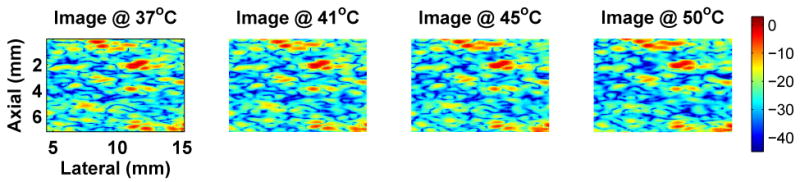
Typical variation of experimental images during heating. One image region is shown from an abattoir specimen of bovine lever for four temperatures in the heating range of 37 to 50°C. Color scale is in dB with dynamic range of approximately 43 dB. Compare to simulated B-mode images of Figure 5.

Figure 3.

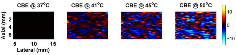
Typical CBE computed from experimental images during heating. These images of the CBE were computed directly from the backscattered energy images of Figure 2. Scale is in dB. Compare to CBE computed from simulated B-mode images in Figure 6.

In general, the CBE computed for each pixel increases or decreases monotonically but is noisy and highly variable. For each image region, CBE was characterized by the means of all negative- and positive-valued pixels in the CBE image. For example, results are plotted in Figure 4 for multiple regions from an in vitro experiment on a bovine liver specimen. Note that these curves are similar to those in Figure 1. Both increasing and decreasing pixels are present; the range of variation is similar; and the changes are generally monotonic.

Figure 4.

Average of positive and negative CBE computed for multiple regions in motion-compensated images of a bovine liver specimen, after Arthur et al. (2005).

Methods: Simulation of Images for Temperature-Dependent Scatterer Populations

The single-scatterer approach used previously in the theoretical model has guided our experimental methods to date. To extend that model to multiple scatterers and to the images that result from their echoes, we have developed methods for simulating images from populations of scatterers with temperature dependence modeled as in the previous single-scatterer work.

Linear Systems Model of Image Formation

Our physical model for image formation combines a linear model for the radio frequency (RF) image with a discrete-scatterer model for the tissue medium (Trobaugh and Arthur 2000). The linear model is commonly used; it can be derived directly from the wave equation and can be used to represent nearly all of the imaging systems in use today (Trobaugh 2000; Wright 1997; Jensen 1999; Macovski 1983). The imaging system is characterized by its point-spread function (PSF), h(r), in general a function over 3-D space, r. For the sake of simplicity, we assume in this work that the imaging system is spatially-invariant, permitting a convolution representation of image formation,

$$\left|i(\text{r},T)\right|=\left|h(\text{r})\ast q(\text{r},T)\right|\hspace{0.17em}$$ (2)

where i(r, T) is a complex representation of the temperature(T)-dependent RF image, modeled as the convolution of the PSF and reflectivity q(r, T), representing the temperature-dependent acoustic properties of the medium. The magnitude of the complex image i(r, T) gives the signal energy as conventionally displayed. In these simulations, the elevation dimension was not considered, and a 2-D PSF was used, approximated as a windowed sinusoid, e.g., h(r) = A(r)e^j2k₀z, where k₀ = ω₀/c represents the wavenumber corresponding to the center frequency, ω₀, of the transducer, and the window A(r) is a 2-D Gaussian function with widths appropriate for the lateral and axial resolution of the imaging system.

The tissue medium is represented acoustically as a collection of discrete scatterers,

$$q(\text{r},T)=\sum _{i=1}^N{q}_i(T)\delta (\text{r}-{\text{r}}_i)$$ (3)

where the ith scatterer has a temperature-dependent reflectivity, q_i(T), and a position, r_i. In general, the discrete representation simplifies analysis and permits a straightforward characterization of the tissue microstructure as a random distribution of points. For this work, scatterer positions are assumed to be random over the image region, and scatterer concentration, in scatterers per cm², determines a number of scatterers per unit area. Scatterer reflectivity was assumed to be proportional to the backscatter coefficient, with temperature dependence modeled as detailed in equation 1 and shown in Figure 1, depending on the scatterer type. Images representing multiple populations of scatterer types with varying temperature dependence can be simulated for those scatterers using equation 2. Details of the simulation parameters and methods are included in the next section.

Simulations

Simulated B-mode images were generated using a procedure detailed previously in a discrete-scatterer model for images of rough surfaces (Trobaugh and Arthur 2000; 2001). In the current work, collections of discrete scatterers were generated to represent lipid and aqueous populations based on associated scatterer concentrations for each. Each scatterer position was generated as a sample of a uniformly-distributed 2D random variable. Then for each temperature, reflectivity was adjusted for each scatterer according to the appropriate temperature dependence curve; the RF image was computed using the discrete scatterers and system PSF; a complex-valued representation of the RF image was computed using the Hilbert transform; envelope detection was then performed by taking the magnitude of the complex-valued image.

Simulations were guided by experimental images such as those in Figure 2, which were obtained with the Terason system using a 7MHz, 128-element, linear array transducer. The system PSF was modeled as in (Trobaugh and Arthur 2000; 2001), with a center frequency of 7.0 MHz and spatially-invariant Gaussian envelopes in the axial and lateral dimensions with a lateral beam width of 1 mm (full-width, half-maximum (FWHM)), and axial width of approximately 0.2 mm. PSF widths were chosen based on comparison with the measured PSF of the Terason system (via an image of a point-like target at approximately 4 cm, a typical depth of the target). Gaussian random noise was added to RF images at various levels to explore its contribution to CBE.

In our investigation, we used varying values for scatterer concentration for aqueous and lipid populations. All results were generated with a total concentration of 2000 scatterers/cm² with reflectivity for all scatterers equal to unity at 37°C. Baseline results were generated with lipid and aqueous scatterer populations with relative concentrations of 2:1 aqueous-to-lipid. These parameters were chosen as a baseline to match CBE approximately to experimental results.

Results

Simulation methods were used to explore effects of region size, SNR, and scatterer population on CBE. In Figure 5, a region from a simulated B-mode ultrasound image is shown at multiple temperatures between 37 and 50°C. These images can be compared to the experimental images of Figure 2. Note that the images vary subtly as temperature is increased, as in the experimental images. Figure 6 includes temperature-dependent CBE images computed from the simulated B-mode images. The nature and extent of variation is quite similar to that computed from experimental images as shown in Figure 3.

Figure 5.

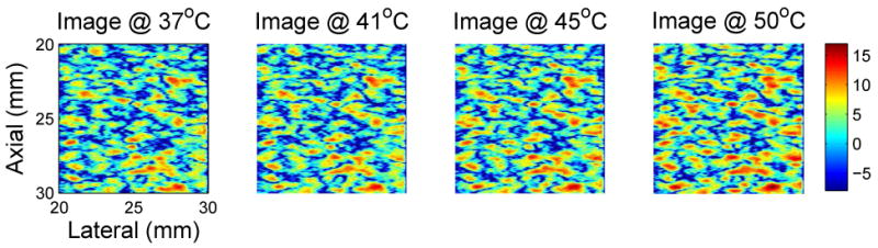
Typical simulated B-mode images generated over the 37 to 50°C temperature range for temperature-dependent scatterers. These images were generated using populations of lipid and aqueous scatterers with the lipid concentration twice that of the aqueous population. Region size is 1cm², and the SNR is approximately 19 dB. Images are log-compressed, with color scale in dB. Compare to experimental images of Figure 2.

Figure 6.

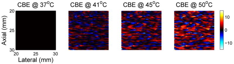
Typical images of CBE over the hyperthermia temperature range. CBE was computed from the simulated B-mode images shown in Figure 5, referenced to the image at 37°C. Color scale is in dB. Compare to experimental images of CBE in Figure 3.

As in our previous analysis of experimental images (Arthur et al. 2005b), CBE images were computed from envelope-detected B-mode images by squaring and averaging with a 3 × 3 moving average filter. CBE over an image region was characterized in three ways: average over those pixels with positive CBE; average over pixels with negative CBE; and the standard deviation of CBE over all pixels. Figure 7 shows typical results for these three CBE parameters for simulated B-mode images with a 2:1 ratio of aqueous to lipid scatterers and no additive noise. CBE is indeed monotonic and covers a range similar to that in previous experiments.

Figure 7.

CBE for 37 to 50°C computed from simulated B-mode images without additive noise.

The CBE curves shown in Figure 7 indicate similar excursions to those generated from experimental images, but the curves are much smoother than the experimental data. Figure 8 shows CBE curves generated from the same RF images as in Figure 7 when Gaussian noise was added to the image. Fluctuation along the curves is quite similar to that in the experimental CBE curves, and note also that the experimental curves often include a sharp increase (or decrease) at the first temperature step, e.g., the jump in CBE from 37.0 to 37.5°C, which is replicated in the simulation results when noise is added. This jump is always present in both experiment and simulation, with an extent that depends primarily on the SNR.

Figure 8.

CBE for 37 to 50°C computed from simulated B-mode images with additive noise.

The plots in the center of Figure 9 show results for 25 different simulations with the same scatterer concentrations and noise levels as in Figures 7 and 8. Note that curves are generally monotonic, with some fluctuation, and cover a similar range, but the individual curves vary substantially, more than 0.5 dB at 50°C. This variation presents a fundamental limitation on the repeatability of CBE measurements and, thus, the potential accuracy of temperature estimation. Determination of primary factors that influence this variation is critical to useful temperature imaging.

Figure 9.

CBE for multiple trials and with change in size of the region.

The three sets of plots in Figure 9 also show the impact of the image region size on CBE and its variation. The smallest region (0.5×0.5cm²) produces significant variation in curves for each of the CBE measures, representing over 1dB at 50°C. The large region, at 1×3cm², produces significantly less variation, ranging over less than 0.5 dB. This size is significant because it represents approximately the same image volume that would be represented for 1cm³ of tissue (based on measured elevation resolution, about 3mm, of our experimental imaging system, indicating roughly 3 independent measurements per centimeter), our goal for spatial resolution in a technique for temperature imaging.

Typical variation of these CBE curves can be quantified for a given region size, SNR, and scatterer population by generating multiple CBE results as in each part of Figure 9 and then computing the mean and standard deviation over all trials. Figure 10 shows the same results as Figure 9 but displayed in terms of the mean and standard deviation at each temperature. For each of the three region sizes, curves are plotted for the three CBE measures. In this case, the mean, or average, curve might be used as a calibration for estimating temperature from subsequent CBE measurements. The standard deviation signifies the expected variation for a given measure and region size, i.e., increasing the region size reduces variation in CBE measurements.

Figure 10.

CBE (mean ± std of 25 trials) for regions of varying size.

Figure 11 shows the same results as Figure 10 but organized by CBE measure. Region size does not change the character of each curve significantly. Its impact is noticed primarily in the standard deviation. In contrast, Figure 12 shows significant variation that can occur in the average CBE curves due to changes in the scatterer populations. Three configurations were included: (1) equal concentrations (1000 scatterers/cm²) of lipid and aqueous scatterers, (2) concentration for lipid scatterers half that of the aqueous, and (3) a population of scatterers with temperature dependence randomly distributed between the prediction for lipid and aqueous scatterers (concentration of 2000 scatterers/cm²). Note that the maximum of all three curves varies significantly depending on which scatterers are present.

Figure 11.

Variation (mean ± std of 25 trials) with region size of three possible CBE parameters.

Figure 12.

Variation (mean ± std of 25 trials) with tissue type of three possible CBE parameters. N_aq/N_lip denotes the ratio of aqueous to lipid scatterers assumed.

Figure 13 shows variation in the CBE curves when the additive noise level is varied to achieve variation in the SNR, measured as the ratio of root-mean-square (rms) signal and noise levels and expressed in decibels (dB). The initial CBE value (at 37.5°C in these figures) is clearly dependent on the SNR, as are the slope of the average CBE curve and the standard deviation over the 25 trials shown.

Figure 13.

Variation (mean ± std of 25 trials) with noise level of three possible CBE parameters.

Results are tabulated in Table 1 for CBE at 44°C, a typical target heating temperature for hyperthermia temperature. Potential accuracy of temperature estimation was estimated as twice the standard deviation (computed from 25 results and shown as the error bar in previous figures), to contain approximately 95% of the results assuming a normal distribution. Accuracy was converted from dB (standard deviation of the CBE measure) to °C based on the slope of the CBE curve (dB/°C)at 44°C.

Table 1.

Accuracy (95%) in °C for estimating temperature at 44°C in configurations tested with simulation, assuming normal distribution with computed standard deviation and slope (dCBE/dT) of CBE as function of temperature. N_aq/N_lip denotes the ratio of aqueous to lipid scatterers assumed. Values marked baseline were used while varying other parameters, e.g., simulations for varying region size employed a 2:1 aqueous-to-lipid ratio and SNR of 19dB.

	Mean + CBE	Mean - CBE	STD CBE
Scatterer Population	Accuracy (±°C)	Accuracy (±°C)	Accuracy (±°C)
Naq/Nlip = 2 (baseline)	0.716	1.385	0.971
Naq/Nlip = 1	0.897	1.649	1.116
Random f(T)	0.612	2.222	1.227
Signal-to-Noise Ratio
13.5dB	0.917	1.839	1.175
19dB (baseline)	0.716	1.385	0.971
33dB	0.907	1.144	0.768
Region Size (cm2)
.5×.5	1.485	2.291	1.817
1×1 (baseline)	0.716	1.385	0.971
1×3	0.488	0.768	0.583

As an example of temperature estimation, results are shown in Figure 14 for calibrating a tissue, estimating temperature, and characterizing results. These results are for the baseline configuration with twice as many aqueous as lipid scatterers, a 1×1cm² image region, and SNR in the middle of the reported range. The plots on the left show a calibration CBE curve, generated as the average curve for mean of the positive CBE (average over 25 trials and shown with standard deviation error bars). The middle plots show estimates of temperature for 25 trials, in which images were simulated as before but computed values of CBE were used to estimate temperature according to linear interpolation using the calibration curve. The plots on the right show the average and standard deviation of the estimates. On average, the estimates are accurate to within 0.1°C. For the estimates at 44°C two standard deviations represents approximately 0.72°C, equivalent to the accuracy prediction shown in Table 1. Note from the plots on the right that the accuracy depends on temperature, and is even better for temperatures under 44°C but worse at higher temperatures.

Figure 14.

Use of mean CBE curve (left, from simulated B-mode images) for calibration and estimation of temperature (center) from subsequent simulated B-mode images, resulting in estimate mean and standard deviation (right).

Discussion

A primary contribution of this simulation model is the ability to investigate the change in backscattered ultrasound energy associated with echoes resulting from multiple scatterers. These results for simulated echoes from multiple scatterers showed CBE consistent with experimental results. This confirmation of the experimental results strengthens our belief that the CBE measurements are based in physical changes rather than measurement artifact, and suggests that our theoretical model for the temperature dependence of an individual scatterer can be extended effectively to tissue media consisting of multiple scatterers of varying types.

Effects of region size, tissue composition, and SNR are difficult to isolate and characterize in experimental situations but are straightforward to separate with this simulation model. The results presented here show clearly the importance of considering region size and SNR in characterizing CBE as a function of temperature. Tissue composition was described in these simulations in a relatively simplistic way, but significant variation in the average CBE curve results even with these simple tissue models of randomly distributed lipid and aqueous scatterers. In using CBE to estimate temperature, e.g., based on the average CBE curve, such variation would result in significant error in temperature. This problem may be overcome by calibrating for a particular tissue type, e.g., muscle of the chest wall, if the acoustic structure of that tissue is consistent across specimens.

Our ultimate objective is to generate quantitative 3D images of temperature, with performance measured in terms of the achievable temperature accuracy for a given spatial resolution. Our stated temperature estimation specification has been to achieve 0.5°C accuracy over 1cm³ volumes. Table 1 quantifies the simulation results by the factor investigated and the CBE parameter explored. These results show clearly the critical importance of a large region for getting accuracy less than 0.5°C. As computed in this work, accuracy depends on the standard deviation and the slope of the CBE curve (the sensitivity of CBE to temperature increase). Accuracy is better, i.e., error is smaller, in situations with either a lower standard deviation or greater sensitivity. From this table, especially poor accuracy is expected for a small region size (due to high standard deviation), and, in most configurations, for the mean of negative CBE (due to low variation in this CBE curve).

The inclusion of additive Gaussian random noise in the simulations helped to explain much of the nature of experimental CBE curves generated previously, specifically the initial jump in CBE and the fluctuation along the curve. This behavior is due at least in part to the characterization of CBE as a ratio of two measurements. When the rms noise, i.e., its standard deviation, is a significant fraction of the rms signal, the computed ratio will vary greatly over multiple measurements. As the SNR increases, this variation decreases. This effect is evident in simulations at varying SNR, with the initial jump in CBE reduced with increasing SNR. Fluctuation along individual curves is also reduced with an increase in SNR. The standard deviation shown as error bars in Figure 13 only partly reflects this reduced fluctuation because shifts in the individual CBE curves also contribute to the overall variation. Similarly, changing noise level can have unexpected consequences; the mean of positive CBE curve improved for a moderate noise relative to lower and higher values. In this case, reducing the noise increases the slope but also increases the standard deviation. Note from Figure 13 that the noise-dependent variation in curve slope is least at 44°C, thus this result may occur only around this temperature.

The simulation model and these results have clarified the importance of some of the factors affecting temperature estimation using CBE. Other choices for tissue type could be explored, including other scatterer types and distributions of those scatterers. The uniform distribution used to date for the scatterers is computationally convenient but presumably different from the true acoustic properties of biological tissue and may have exaggerated the impact of tissue type and the resulting variation in CBE curves. We are currently producing histology samples for tissue in associated heating experiments to investigate relative concentrations of various scatterer types, which may be incorporated into our simulation model. While simulations have made some investigations easier, however, others such as robustness of CBE for a given tissue type may be more easily accomplished in experiments.

Use of CBE for temperature imaging to monitor hyperthermia treatment requires careful treatment of other factors such as tissue motion, heterogeneous heating, and perfusion. In experimental images, tissue motion, whether real or apparent, can have a significant effect on CBE. Methods for motion compensation have been developed and applied previously (Arthur et al. 2005b). Validation and refinement of those methods in this simulation environment will be important, where conditions can easily be controlled. With this ability, we can determine motion-related errors that would be expected in estimating temperature based on CBE. In vivo experiments and analysis conducted with mouse models confirm our basic CBE findings in the presence of perfusion. Experiments are planned to extend this work to humans and cases of heterogeneous heating.

Conclusions

Our model for simulating temperature dependence in backscattered ultrasound for varying populations of scatterers has been shown to produce ultrasound images, images of CBE, and mean CBE curves consistent with those obtained from images in experimental heating arrangements. This model provides the basis for examining significant issues relevant to temperature imaging based on ultrasonic CBE such as effects of image noise on measured CBE, effects of scatterer type and distribution on CBE, effects of motion on CBE and limitations of motion-compensation techniques, and accuracy of temperature estimation, including tradeoffs between temperature accuracy and available spatial resolution.

References

- Arthur R, Straube W, Starman J, Moros E. Noninvasive temperature estimation based on the energy of backscattered ultrasound. Medical Physics. 2003;30:1021–1029. doi: 10.1118/1.1570373. [DOI] [PubMed] [Google Scholar]
- Arthur R, Straube W, Trobaugh J, Moros E. Noninvasive estimation of hyperthermia temperatures with ultrasound. International Journal of Hyperthermia. 2005;21:589–600. doi: 10.1080/02656730500159103. [DOI] [PubMed] [Google Scholar]
- Arthur R, Trobaugh J, Straube W, Moros E. Temperature dependence of backscattered ultrasonic energy in motion-compensated images. IEEE Transactions on Ultrasonics, Ferroelectrics and Frequency Control. 2005;52:1644–1652. doi: 10.1109/tuffc.2005.1561620. [DOI] [PubMed] [Google Scholar]
- Falk M, Issels R. Hyperthermia in oncology. International Journal of Hyperthermia. 2001;17:1–18. doi: 10.1080/02656730150201552. [DOI] [PubMed] [Google Scholar]
- Jensen J. Technical report. Technical University of Denmark; 1999. Linear description of ultrasound imaging systems, notes for the international summer school on advanced ultrasound imaging, technical university of denmark july 5 to july 9, 1999. [Google Scholar]
- Jones E, Oleson J, Prosnitz L, Samulski T, Vujaskovic Z, Yu D, Sanders L, Dewhirst M. Randomized trial of hyperthermia and radiation for superficial tumors. Journal of Clinical Oncology. 2005;23:3079–3085. doi: 10.1200/JCO.2005.05.520. [DOI] [PubMed] [Google Scholar]
- Macovski A. Medical Imaging Systems. Prentice-Hall; 1983. [Google Scholar]
- Moros E, Corry P, Orton C. Point/counterpoint: Thermoradiotherapy is underutilized for the treatment of cancer. Medical Physics. 2007;34:1–4. doi: 10.1118/1.2404790. [DOI] [PubMed] [Google Scholar]
- Straube W, Arthur R. The temperature dependence of backscattered ultrasonic power normalized for use in hyperthermia. Utrasound in Medicine and Biology. 1994;20:915–922. doi: 10.1016/0301-5629(94)90051-5. [DOI] [PubMed] [Google Scholar]
- Trobaugh J. PhD thesis. Washington University; St. Louis: 2000. An Ultrasonic Image Model Incorporating Surface Shape and Microstructure and System Characteristics. [Google Scholar]
- Trobaugh J, Arthur R. A discrete-scatterer model for ultrasonic images of rough surfaces. IEEE Transactions on Ultrasonics, Ferroelectrics, and Frequency Control. 2000;47(6):1520–1529. doi: 10.1109/58.883541. [DOI] [PubMed] [Google Scholar]
- Trobaugh J, Arthur R. A physically-based, probabilistic model for ultrasonic images incorporating shape, microstructure and system characteristics. IEEE Transactions on Ultrasonics, Ferroelectrics, and Frequency Control. 2001;48(6):1594–1605. doi: 10.1109/58.971711. [DOI] [PubMed] [Google Scholar]
- Wright J. Image formation in diagnostic ultrasound. Short Course, IEEE International Ultrasonics Symposium. 1997 [Google Scholar]