Improved temporal coding of sinusoids in electric stimulation of the auditory nerve using desynchronizing pulse trains

Abstract

Rubinstein et al. [Hearing Res. 127, 108–118 (1999)] suggested that the representation of electric stimulus waveforms in the temporal discharge patterns of auditory-nerve fiber (ANF) might be improved by introducing an ongoing, high-rate, desynchronizing pulse train (DPT). To test this hypothesis, activity of ANFs was studied in acutely deafened, anesthetized cats in response to 10-min-long, 5-kpps electric pulse trains that were sinusoidally modulated for 400 ms every second. Two classes of responses to sinusoidal modulations of the DPT were observed. Fibers that only responded transiently to the unmodulated DPT showed hyper synchronization and narrow dynamic ranges to sinusoidal modulators, much as responses to electric sinusoids presented without a DPT. In contrast, fibers that exhibited sustained responses to the DPT were sensitive to modulation depths as low as 0.25% for a modulation frequency of 417 Hz. Over a 20-dB range of modulation depths, responses of these fibers resembled responses to tones in a healthy ear in both discharge rate and synchronization index. This range is much wider than the dynamic range typically found with electrical stimulation without a DPT, and comparable to the dynamic range for acoustic stimulation. These results suggest that a stimulation strategy that uses small signals superimposed upon a large DPT to encode sounds may evoke temporal discharge patterns in some ANFs that resemble responses to sound in a healthy ear.

I. Introduction

Speech and other sound stimuli contain information in both their slowly varying envelope and their rapidly varying fine-time structure (Rosen, 1992). Yet, many processing strategies used in today's cochlear implants only deliver envelope information and discard the temporal fine structure. For example, continuous interleaved sampling (CIS) strategies (Wilson et al., 1991) use an envelope detector in each frequency channel to derive waveforms used to modulate carrier pulse trains. These envelope detectors discard the information available in the fine-time structure. The SPEAK strategy used with Nucleus implants (Seligman and McDermott, 1995) also discards the fine structure in each stimulated channel.

Smith et al. (2002) evaluated the relative importance of envelope and fine-time structure information in auditory perception using acoustic stimuli called “auditory chimeras.” The chimeras are sounds which, in each frequency band, have the fine-time structure of one sound, and the envelope of another. Smith et al. found that, with four to eight frequency bands, speech comprehension is better using the envelope information than the information in the fine-time structure. However, for the same number of analysis channels, subjects performed melody identification and sound localization tasks better with the fine-time structure than with the envelope information. These results suggest that modifying cochlear implant processing strategies to include fine-time structure information might improve pitch perception. The fine structure may also be essential for taking full advantage of binaural cues delivered by bilateral implants.

Fine structure information might be delivered to cochlear implants in several ways. The simplest method, already used in some processing strategies, is to deliver an analog representation of the stimulus waveform in each frequency channel. Alternatively, the frequency of a periodic stimulus might be encoded by the rate of a pulse train. Although this method has the disadvantage that signals having different waveforms cannot be distinguished if they have the same fundamental frequency, it was used in early Nucleus processors to encode the fundamental frequency of voice (Tong et al., 1980). Finally, fine structure information might be introduced in a CIS strategy by increasing the cutoff frequency of the envelope detector, or even eliminating it altogether. The rate of the carrier pulse trains would also have to be increased so as to sample the resulting high-frequency modulation waveforms without aliasing.

Both single-unit studies in animals and evoked potential studies in implanted human subjects suggest that neither of the above strategies for delivering fine structure information would, by itself, produce temporal discharge patterns in the auditory nerve resembling those evoked by acoustic stimuli in a normal ear. Auditory-nerve fibers (ANF) encode the fine-time structure of acoustic stimuli in their temporal discharge patterns for frequencies up to 5 kHz (Rose et al., 1967; Johnson, 1980). For example, in response to a pure tone, neurons fire at random multiples of the stimulus period, in that there may be one, two or more cycles between successive spikes (Rose et al., 1967). The stimulus period is thus represented in the ensemble activity of a population of neurons by a stochastic form of Wever's volley principle, even when the stimulus period is shorter than the neural refractory period. This coding scheme is made possible by the ongoing stochastic release of neurotransmitter at inner-hair-cell synapses, and the modulation of this neurotransmitter release by the receptor potential which tracks each cycle of the stimulus waveform.

Because hair cells and their synapses are missing in deaf ears, temporal discharge patterns produced by electric stimulation are very different from normal acoustic responses. Suprathreshold responses to electric pulse trains or sinusoids with frequencies below 500–800 Hz behave nearly deterministically, typically showing one spike discharge on every stimulus cycle (Moxon, 1967; Hartmann et al., 1984, 1990; van den Honert and Stypulkowski, 1987; Parkins, 1989; Javel et al., 1987; Javel, 1990; Javel and Shepherd, 2000). Such entrainment also occurs for sinusoidally modulated electric pulse trains similar to stimuli produced by CIS processors (Litvak et al., 2001). Moreover, the temporal precision of discharges evoked by such low-frequency electric stimuli is much higher than with acoustic stimulation (Hartmann et al., 1984, 1990; Javel, 1990; Javel and Shepherd, 2000). For example, whereas spikes are distributed over most of one-half cycle in response to a pure tone, they only occupy a small fraction of the stimulus cycle for electric sinusoids, thereby inadequately representing the sinusoidal wave shape (Hartmann et al., 1984; van den Honert and Stypulkowski, 1987). In fact, temporal discharge patterns for electric sinusoidal, triangular and square waves of the same frequency are surprisingly similar considering that these stimuli have very different spectra (van den Honert and Stypulkowski, 1987; Parkins, 1989).

Further issues arise at higher frequencies (>500–800 Hz) where neural refractoriness prevents fibers from discharging on every cycle of the electric stimulus. With both sinusoidal and pulse train stimuli, refractoriness can cause history-dependent changes in response latency, resulting in a neuron discharging at two distinct phases within a stimulus cycle (Parkins, 1989; Javel, 1990; Javel and Shepherd, 2000). Such double-peaked period histograms are not observed for acoustic stimulation above 1000 Hz (Johnson, 1980). Interval histograms are also highly abnormal, demonstrating a tendency for spikes to occur at regular intervals, even for high-frequency (>1000 Hz) stimulation (Parkins, 1989; Dynes and Delgutte, 1992). In some cases, ANFs fire exactly on every other cycle or even at higher multiples of the stimulus period (Javel, 1990; Javel and Shepherd, 2000). This tendency is also apparent in measurements of electric compound action potentials (ECAPs) from cochlear implant users (Wilson et al., 1997). Specifically, in response to a 1-kpps electric pulse train, ECAPs alternate between strong and weak responses to each pulse for up to 100–200 ms after stimulus onset. This alternation suggests that, while most ANFs respond to the first pulse, they are in a refractory state during the second pulse and only respond again to the third pulse. If most fibers fire together on every other cycle, then the auditory nerve population represents half the stimulus frequency rather than the actual frequency. In summary, neural refractoriness, the narrow dynamic ranges, excessively high discharge rates, and exaggerated synchrony combine to make the temporal coding of electric stimuli highly unnatural compared to normal acoustic stimulation, particularly for frequencies above 500 Hz.

Rubinstein et al. (1999b) proposed that the temporal coding of stimulus waveforms in cochlear implants might be improved by introducing an ongoing, high-frequency, desynchronizing pulse train (DPT) in addition to the signal produced by the speech processor. The purpose of a DPT is to amplify noise in sodium channels so as to produce more stochastic responses similar to those of spontaneously active fibers. In a companion paper (Litvak et al., 2003b), we recorded ANF responses to a 10-min, 5-kpps DPT. We found that, after 1–2 min of continuous stimulation, the DPT produced activity that, in many fibers, resembled spontaneous activity in a healthy ear. Several types of responses to the DPT were identified. Some fibers (roughly 50%) only responded transiently to the DPT, while the others showed a sustained response throughout 10 min of DPT stimulation. For the sustained responders, the “pseudo-spontaneous” activity evoked by the DPT had broadly distributed interspike interval distributions and appeared to be uncorrelated from fiber to fiber. Some interval histograms (25%) had an exponential shape, as does normal spontaneous activity; however, the majority of sustained responses had nonexponential interval histograms, particularly if they discharged at very high rates.

In this paper, we directly test the hypothesis that a DPT improves the representation of the fine-time structure in the temporal discharge patterns of ANFs for sinusoidal stimuli. There are at least three ways in which a DPT could make responses to electric stimuli better resemble acoustic responses in a healthy ear. First, a DPT could desynchronize stimulus-evoked activity across-fibers. For higher-frequency (>500 Hz) stimuli, desynchronization may allow different neurons to discharge on different stimulus cycles, thereby allowing volley coding of frequency. By simultaneously recording from pairs of fibers, we showed that such desynchronization does in fact occur after a few seconds of DPT stimulation (Litvak et al., 2003b).

Second, a DPT may allow small electric signals to be encoded as modulation of ongoing DPT-evoked pseudo-spontaneous activity, much as normal acoustic responses of most ANFs are effectively modulations of ongoing spontaneous activity. Such modulations of random activity allow faithful transmission of the stimulus waveform in neural discharges by a process akin to stochastic resonance (Yu and Lewis, 1989; Collins et al., 1995; Wiesenfeld and Moss, 1995). If the stochastic nature of the responses could be restored by the DPT, then a similar mechanism may also improve the coding of the stimulus fine-time structure in electric stimulation.

Finally, computer simulations of auditory-nerve fibers suggest that a DPT may lower the threshold and increase the dynamic range to electric stimulation (Rubinstein et al., 1999a). The increased dynamic range is particularly significant when one considers complex stimuli such as vowels. These waveforms contain peaks of widely different heights in each period. A wide dynamic range might allow fibers to represent all of the waveform peaks in their temporal discharge patterns rather than just the largest peak.

Previous tests of the ideas underlying the DPT (Rubinstein et al., 1999b; Wilson et al., 1998) were based on electric compound auditory potential (ECAP) responses, which provide only indirect evidence of single-unit activity. In addition, these studies used short pulse trains (30 ms), which are a poor model of an ongoing DPT. We found that responses to a DPT only reach a near steady state after 1–2 min of DPT stimulation (Litvak et al., 2003b). In this paper, we directly test the hypotheses underlying the DPT by recording from single fibers from the auditory nerve of deafened cats. We focus on responses that occurred after adaptation to a DPT presented for 10 min. We compare temporal discharge patterns of ANFs for sinusoidal modulations of a DPT with normal acoustic responses to pure tones. We also test the hypothesis that the DPT increases the dynamic range by studying responses to sinusoidally modulated DPTs over a range of modulation depths.

Our scheme for encoding acoustic signals into electric waveforms differs somewhat from that used by Rubinstein et al. (1999b) in their original formulation of the DPT idea. In that paper, an analog electric sinusoid was directly superimposed upon a DPT; here we encode the sinusoid as a small modulation of a DPT. This coding scheme assumes that neural responses to a high-rate pulse train with low modulation depth are similar to those elicited by the superposition of a large, unmodulated DPT and a small, highly modulated pulse train as might be produced by a CIS processor (Fig. 1). This assumption is a mathematical identity if the same pulse train is used for both the DPT and the CIS carrier. It may hold more generally if the time constant of the neural membrane is large compared to the intervals between pulses. In this scheme, modulation depth is proportional to the amplitude of the sinusoidal stimulus for small modulations. The differences between the present scheme and the Rubinstein et al. (1999b) original strategy will be further considered in Sec. IV.

FIG. 1.

The stimuli used in our experiments are pulse trains with low modulation depths (right). These stimuli can be thought of as the superposition of a large, unmodulated DPT (bottom left) and a small, fully modulated pulse train (top left) similar to the signals produced by CIS processors.

II. Methods

The animal preparation, electrical stimulation, and recording methods are described in the companion paper (Litvak et al., 2003b). Briefly, cats were anesthetized with dial in urethane (75 mg/kg), then deafened by co-administration of kanamycin (subcutaneous, 300 mg/kg) and ethacrinic acid (intravenous, 25 mg/kg) (Xu et al., 1993). As described in detail in the companion paper (Litvak et al., 2003b), most of the animals had some residual hearing in the nonimplanted ear. To minimize the effect of residual hair cells in these preparations, we only report responses from neurons with no spontaneous activity in the absence of a DPT. Two intracochlear stimulating electrodes (400 mm Pt/Ir balls) were inserted into the cochlea through the round window. One electrode was inserted approximately 8 mm and was used as the stimulating electrode. The other electrode was inserted just inside the round window and served as the return electrode.

Standard techniques were used to expose the auditory nerve via a dorsal approach (Kiang et al., 1965). We recorded from single units in the auditory nerve using glass micropipettes filled with 3M KCl. For small modulation depths, most of the stimulus artifact could be removed online using a digital signal processor implementing a moving average filter whose length matched the 0.2-ms pulse period. Neural responses were also recorded digitally with a sampling rate of 20 kHz for off-line analysis. Methods used to remove the stimulus artifact from these records are described in Appendix A.

A. Stimuli

We conducted a neural population study by investigating responses to a single DPT level for each animal. To ensure that a large fraction of fibers would respond to the DPT, the DPT level was set at 8–10 dB above ECAP threshold, as described in detail in the companion paper (Litvak et al., 2003b).

We studied responses to small (modulation depth ≤15%) sinusoidal modulations of the DPT. Figure 3 (top) schematizes the envelope of the electric stimuli. The carrier was a 5-kpps train of biphasic pulses (cathodic/anodic, 25 μs per phase). In order to acquire responses to both the unmodulated DPT and modulations of the DPT for several modulation depths and frequencies, the stimulus was composed of alternating modulated (400 ms) and unmodulated (600 ms) segments.¹ Modulation depth and, in some cases, modulation frequency was changed on each successive segment. Modulation depth was varied from 0.5% to 15%, while modulation frequency was either 104, 417 or 833 Hz. The entire sequence of modulated and unmodulated segments had a 5–12-s period, and was repeated continuously for 10 min or until contact with the fiber was lost.

FIG. 3.

The top panel shows one cycle of the electric pulse train stimulus (5 kpps, 2.5 mA 0-p) to which a 417-Hz sinusoidal modulation was applied every second for 400 ms. Modulation depth ranged from 0.5% to 11%, and the entire sequence of modulations was repeated every 5 s for 10 min. The left panel of the middle row shows a period histogram (bin width 2.4 ms) locked to the 5-s modulation cycle for one auditory-nerve fiber. For comparison, the right two panels of the middle row show the response pattern of an ANF (CF=650 Hz) from a healthy ear to a 440-Hz pure tone at 5 and 45 dB above threshold. The bottom panels show the period histograms computed from responses during the electric modulations (left) and the acoustic pure tone (right). The gray line shows a sinusoidal waveform for comparison.

Modulation was applied such that the mean amplitude of the carrier pulses was the same during modulated and unmodulated segments. Specifically, during modulation, the envelope was defined as A · (1 + m · sin(2πf_mt)), where f_m is the modulation frequency, A is the amplitude of the unmodulated DPT, and m is the modulation depth. The modulation period was always an integer multiple of the 0.2-ms carrier period to avoid beating, and the modulation phase was chosen so that the peak of the modulation waveform always coincided with a carrier pulse.

B. Analysis

Responses collected during the unmodulated DPT segments were used to classify each fiber using the same scheme as in the companion paper (Litvak et al., 2003b). Some fibers exhibited only a transient response to the DPT, and adapted to near zero (<5 spikes/s) discharge rate after 100 s of DPT stimulation. We will refer to these fibers as “transient DPT responders.” Fibers that responded to the unmodulated segments over the entire stimulus duration will be referred to as “sustained responders.”

Litvak et al. (2003b) further used interval histograms to characterize the temporal discharge patterns of sustained responders. We found that, while some responses had nearly exponential interval histograms, others had strongly nonexponential interval histograms. The degree of “exponentiality” of the histogram was quantified using an Interval Histogram Exponential Shape Factor (IH-ExpSF) (Litvak et al., 2001). The IH-ExpSF is computed by first fitting the interval histogram with both a single exponential and, piecewise, by three exponentials. The root mean squared (rms) error of each fit to the data is then determined, and the IH-ExpSF defined as the ratio of the rms error for the piecewise fit to that for the single exponential fit. The IH-ExpSF for samples from a stationary Poisson process is approximately 1.

C. Stochastic threshold model

As a concise way of summarizing the data, we developed a simple functional model of responses of ANFs to modulations of a DPT (Fig. 2). The model takes as input the modulation waveform m(t). For a sinusoidal modulator, m(t) = m · sin(2πf_mt), where f_m is modulation frequency, and m is modulation depth. A spike is produced by the model whenever m(t) crosses a noisy threshold. The threshold is the sum of a deterministic term and a noise term. To account for the refractory properties of ANFs, the deterministic component of threshold θ_n(t) depends on the time since the preceding spike t_i according to Eq. (1), also used by Bruce et al. (1999):

FIG. 2.

Stochastic threshold model (STM) of ANF responses to modulations of a DPT. The model takes as input the modulation waveform m(t) and produces a spike whenever the input crosses a noisy threshold. The output of the model is a set of spike times {t_i}. The threshold is the sum of a Gaussian noise term n(t) and a deterministic term θ_n(t) which depends on the time since the previous spike. The only free parameters in the model are the resting threshold θ₀ and the noise amplitude σ.

$$\begin{array}{lll}{\theta }_n(t)& =& {\theta }_0\hspace{0.17em}·\hspace{0.17em}r(t)\hfill \\ & =& {\theta }_0\hspace{0.17em}·\hspace{0.17em}\{\begin{array}{l}\infty ,\hspace{0.17em}\hspace{0.17em}\hspace{0.17em}t-t_i<0.6\hspace{0.17em}\hspace{0.17em}\text{ms},\hfill \\ 1+0.97exp[-(t-t_i)/1.32\hspace{0.17em}\hspace{0.17em}\text{ms}],\hfill \\ \hspace{0.17em}\hspace{0.17em}\hspace{0.17em}\hspace{0.17em}\hspace{0.17em}t-t_i\ge 0.6\hspace{0.17em}\hspace{0.17em}\text{ms}.\hfill \end{array}\hfill \end{array}$$ (1)

The threshold recovery function r(t) was chosen to fit the absolute and relative refractory periods of electrically stimulated ANFs (Dynes, 1995). For the noise term, we used computer-generated zero-mean, white Gaussian noise with standard deviation σ. Because the model was simulated using 0.2-ms time steps, the noise bandwidth was effectively 2500 Hz. Because the noisy threshold is the critical element of the model, we refer to this model as the stochastic threshold model (STM).

We computed responses of the STM to sinusoidal modulators of different frequencies and modulation depths. The conditional probability that a model neuron fires at time t given that the last spike occurred at t_i is

$$p_f(t)=\Gamma \left(\frac{m}{\sigma }\hspace{0.17em}·\hspace{0.17em}sin(2\pi f_{m}t)-\frac{{\theta }_0}{\sigma }r(t-t_i)\right),$$ (2)

where Γ is the cumulative Gaussian distribution, and r(t) is the recovery function described by Eq. (1). For an unmodulated DPT (m = 0), the pseudo-spontaneous discharge rate (the discharge rate during the unmodulated DPT) is entirely determined by the threshold-to-noise ratio θ₀/σ. For nonzero values of m, the discharge rate depends on the ratio m/σ as well. These two ratios entirely determine the model response to sinusoids.

III. Results

A. Basic response characteristics

Our results are based on 68 responses recorded from 62 auditory-nerve fibers in five cats to sinusoidally modulated electric pulse trains. Each record included responses to a series of modulated segments with different modulation depths and, in some cases, different modulation frequencies. For 28 of these records, the fiber responded to the unmodulated DPT segments at a discharge rate above 5 spikes/s throughout the stimulus duration. For the other 40 records, the fiber stopped responding to the unmodulated DPT after 1–2 min of stimulation, although it still responded to some of the modulated segments. The percentage of transient responders in the present data sample is somewhat larger (59% vs 46%) than in the larger sample from ten cats described in the companion paper (Litvak et al., 2003b), and the difference is statistically significant (p = 0.0247, binomial exact test). We attribute this difference to a combination of biases in data collection (the silent responses of transient responders to unmodulated DPTs were sometimes discarded) and individual differences among animals (some animals had a high proportion of transient responses). In the following, we describe only the responses that occurred after 50 s of stimulation so that the data would reflect the effects of adaptation to the DPT.

Figure 3 shows the response of an auditory-nerve fiber to a DPT that was sinusoidally modulated at 417 Hz for 400 ms every second. Modulation depth was increased from 0.5% to 11% on each successive modulated segment. The entire 5-s cycle of five modulation depths was repeated for 10 min. During the unmodulated segments, the pseudo-spontaneous discharge rate was 48 spikes/s, and the interspike interval distribution was nearly exponential (IH – ExpSF = 0.99).

The left panel in the middle row shows the discharge rate as a function of time from the onset of the 5-s stimulus cycle. Average discharge rate grows monotonically with increasing modulation depth. For modulation depths between 0.5% and 5%, the discharge rate stays below 300 spikes/s, in the range appropriate for responses to tones in a healthy ear (Kiang et al., 1965; Liberman, 1978). At the largest modulation depth (11%), the discharge rate exceeds the rates seen in Liberman's data.

The right two panels in the middle row show the response patterns of a high spontaneous-rate fiber in a healthy ear to 440-Hz tone bursts at 5 and 45 dB above threshold (McKinney and Delgutte, 1999). Consistent with classic descriptions (Westerman and Smith, 1984), the discharge rate decreases rapidly during the first 10 ms of tone-burst stimulation, and this rapid adaptation is followed by slower adaptation with a time constant near 100 ms. In contrast, the responses to modulations of the DPT (left) show a form of slow adaptation, but no sign of rapid adaptation.

The bottom left panel in Fig. 3 shows period histograms locked to the modulator frequency computed from responses during the modulated DPT segments. The period histogram for a modulation depth of 0.5% is already almost fully modulated, indicating exquisite sensitivity to modulation. At this modulation depth, there is little or no increase in discharge rate over that evoked by the unmodulated DPT. Thus, synchrony to the stimulus is already large at a modulation depth that evokes no noticeable increase in average rate over the response to the unmodulated DPT. Similar behavior is found in responses of high-spontaneous ANFs to pure tones (Johnson, 1980).

As the modulation depth increases, responses become more precisely phase locked. For a modulation depth of 1%, the period histogram approaches a half-wave rectified sinusoid, suggesting that the modulator waveform is accurately represented in the temporal discharge patterns. For this modulation depth, the period histogram resembles those in response to a pure tone in a healthy ear (Fig. 3, bottom right). For modulation depths above 2.5%, however, the period histogram consists of a very sharp mode restricted to a small fraction of the stimulus cycle, and does not resemble the response to a pure tone at any level. These hyper-synchronized responses resemble responses to sinusoidal electric stimulation without a DPT (Hartmann et al., 1984; van den Honert and Stypulkowski, 1987).

B. Temporal discharge patterns for exponential fibers

Figure 4 shows period histograms computed from responses to 104, 417, and 833 Hz sinusoidal modulations of the DPT for another ANF. Modulation depth was varied from 0.5% to 10%. During the unmodulated segments, this fiber had a pseudo-spontaneous discharge rate of 54 spikes/s and an exponential interspike interval distribution.

FIG. 4.

Period histograms (bin width 0.2 ms) computed from the response of an auditory-nerve fiber to sinusoidally modulated pulse trains at three different frequencies (columns) and five modulation depths (rows). During the unmodulated segments of the DPT, this fiber had a pseudo-spontaneous discharge rate of 54 spikes/s, and its interval histogram had a nearly exponential shape (IH – ExpSF = 0.97). Numbers in each panel are the average discharge rate (in spikes/s) and the synchronization index to the modulation. The vertical axis is in spikes/s.

For all modulation frequencies, stimuli with modulation depths below 5% evoked average discharge rates below 300 spikes/s, in the range reported for ANFs in normal ears for pure-tone stimulation (Liberman, 1978). In addition, the synchronization index was always below 0.9, consistent with acoustic responses to pure tones. The nearly sinusoidal shape of the period histograms for modulation depths below 2.5% suggests that the modulation waveform is accurately represented for all three modulation frequencies.

At 10% modulation depth, the discharge rates in responses to 417- and 833-Hz modulators exceed those seen in a normal ear. At this high modulation depth, the period histogram for the 104-Hz modulator reveals multiple peaks for each cycle, and this is seen for 5% modulation as well. Unlike the “peak splitting” observed in responses of ANFs to low-frequency tones (Johnson, 1980; Kiang and Moxon, 1972) which always occurs on opposite phases, both peaks of the responses to the electric stimulus occur during the same half-cycle of the modulator. Similar double-peaked responses have been reported for sinusoidal electric stimulation without a DPT (Hartmann et al., 1984; van den Honert and Stypulkowski, 1987).

Interspike interval histograms were also examined to determine whether they resemble those evoked by pure tones in a healthy ear. Figure 5 shows the interval histograms that correspond to the period histograms in Fig. 4. Interval histograms for a 440-Hz pure tone in a normal ear are also shown for comparison. Phase locking to the stimulus can be seen in these histograms as the clustering of intervals around integer multiples of the stimulus period (dashed lines).

FIG. 5.

The first three columns show the interval histograms corresponding to the period histograms in Fig. 4. The numbers in each panel are the average discharge rates in spikes/s. Vertical dashed lines mark multiples of the stimulus period. The vertical axis represents the number of intervals per bin. For comparison, the rightmost column shows interval histograms of an ANF (CF = 650 Hz) from a healthy ear for a 440-Hz pure tone at 5 and 45 dB above threshold.

For modulation depths below 5%, interval histograms for the modulated DPT resemble acoustic responses in that they have exponential envelopes, and show several modes at multiples of the modulation period. One exception is the response to the 417-Hz modulator at 2.5% modulation depth, where the sharp interval mode at twice the stimulus period means that spikes occur on every other stimulus cycle. However, this response pattern is unusual for this modulation frequency and depth. Detailed examination of the interval histograms for modulation depths below 2.5% reveals an additional difference between DPT responses and normal responses to pure tones. Interval histograms for pure tone stimuli always show a mode at the tone's period for frequencies below 1000 Hz (Rose et al., 1967). In contrast, responses to the 417-Hz modulated electric pulse train show no mode at the modulation period; instead, the earliest mode occurs at twice the period. Such lack of a mode at the period has also been observed in response to both electric sinusoids and sinusoidally-modulated pulse trains presented without a DPT (van den Honert and Stypulkowski, 1987; Litvak et al., 2001).

For 10% modulation depth the interval histograms of responses to electric stimulation differ strongly from normal responses to tones. In response to the 104-Hz modulator, the fiber fired twice on each modulation cycle, so that the interval histogram had just two modes, one at 2.3 ms and the other one at 7.3 ms. The sum of these two mode locations equals the 9.6-ms modulation period. For 417-Hz modulation, the interval histogram had a single mode at the modulation period, meaning that a spike occurred exactly once per modulation cycle. Such entrainment is not seen in normal ANF responses to pure tones (Rose et al., 1967), but is common in electric responses without a DPT. For the 833-Hz modulator, the histogram showed a dominant mode at twice the modulation period, indicating that a spike occurred on nearly every other cycle. This distortion is particularly disturbing, because, if it occurs in many fibers, and these fibers fire in synchrony, then the response of the ANF population would represent a signal at half the actual modulation frequency. A tendency for spikes to occur at integer multiples of the stimulus period for frequencies above 500 Hz has also been observed for pulsatile electric stimulation without a DPT (Javel, 1990; Javel and Shepherd, 2000).

Responses of transient responders, a representative example of which is shown in Fig. 6, contrast sharply with those of sustained responders illustrated in Figs. 3–5. This fiber did respond to modulations of the DPT, even though, after adaptation, it showed no spike discharges to the unmodulated DPT (zero pseudo-spontaneous rate). However, the modulation depth necessary to evoke a significant response exceeded 5%, larger than that for any of the sustained responders. In addition, for the 104- and 417-Hz modulators, the synchronization index was invariably higher than that for pure tone responses in a healthy ear. Regardless of modulation depth, the period histogram poorly represented the sinusoidal modulation waveform. Overall, these responses resemble responses to electric sinusoids presented without a DPT (Hartmann et al., 1984; van den Honert and Stypulkowski, 1987).

FIG. 6.

Period histograms of responses of a fiber that gave a transient response to the unmodulated DPT for three modulation frequencies and four modulation depths. Same format as in Fig. 4.

C. Temporal discharge patterns for nonexponential fibers

For the most part, fibers with nonexponential interval histograms during the unmodulated DPT (Litvak et al., 2001, 2003b) responded to modulations of the DPT in a manner similar to the exponential, sustained responders illustrated in Fig. 3–5, but they also showed some unique features, particularly for very small modulations. For example, the top left panel of Fig. 7 shows the interspike interval computed from responses of a fiber to an unmodulated DPT. The interval histogram is clearly nonexponential and shows a pronounced mode at 3.3 ms. We refer to the location of this mode as the preferred interval. We found that preferred intervals systematically influenced the temporal discharge patterns for small modulations of a DPT. The middle panels of Fig. 3 shows the interval (left) and period (right) histogram for responses to 417-Hz modulation of the DPT at 0.5% modulation depth. The period histogram shows that the response is phase locked to the modulator, yet the first mode of the interval histogram is systematically offset from the modulation period (dotted lines). We refer to the shift of the largest mode in the interval histogram as the mode offset. The direction of the mode offset is towards the preferred interval for the unmodulated DPT. A mode offset is also detectable at 2.5% modulation depth (lower left panel), although it is less pronounced than for 0.5% modulation.

FIG. 7.

Interval (left) and period (right) histograms of a fiber's responses to 417-Hz modulations of the DPT at two modulation depths (0.5% and 2.5%). The nonexponential interval histogram (IH – ExpSF = 0.51) computed from responses during the unmodulated DPT segments is shown on top. The vertical axis represents number of intervals per bin for the interval histograms, and discharge rate in spikes/s for the period histograms.

The mode offsets in interspike intervals of nonexponential units are accompanied by decreased phase locking to the modulator, when compared to exponential units. At 0.5% modulation depth, responses of the nonexponential fiber in Fig. 7 were weakly phase locked to the modulator (synchronization index of 0.24). In contrast, at the same modulation depth, the response of the exponential unit in Fig. 4 was already nearly fully modulated (SI = 0.53). The nonexponential unit also shows reduced phase locking at the 2.5% modulation depth.

Reduced phase locking to a 417-Hz modulator as in Fig. 7 was observed in some, but not all nonexponential fibers. Figure 8 shows the synchronization index to a 417-Hz sinusoidal modulator (0.5% modulation depth) against the interval histogram exponential shape factor (IH-ExpSF) for the unmodulated DPT. For units with IH-ExpSF above 0.8, the synchronization index was uniformly high (between 0.3 and 0.6). In contrast, for units with IH-ExpSF below 0.8, the synchronization index varied widely (from 0.1 to 0.5), and could be as high as those of exponential units in some cases, but much lower in others. The correlation between IH-ExpSF and synchronization index was highly significant (p = 0.007, permutation test).²

FIG. 8.

The left panel shows the synchronization index to a 417-Hz modulator (0.5% modulation depth) as a function of the interval histogram exponential shape factor (IH-ExpSF) for 25 fibers from four cats. The IH-ExpSF was computed based on responses during the unmodulated segments of the DPT. The right panels show interval histograms of responses to the unmodulated DPT for two units with low IH-ExpSF. The vertical dashed lines mark multiples of the modulation period.

The variability in phase locking among nonexponential neurons can be understood from the relationship between the modulation period and the preferred interval for unmodulated DPTs. When the preferred interval is close to the modulation period, synchrony to the modulator is high (Fig. 8, upper inset). In contrast, when the preferred interval does not match the modulation period, synchrony to the modulator is low (lower inset in Fig. 8; see also Fig. 7). This observation suggests that the responses to small modulations of a DPT show an interaction between the stimulus drive and the intrinsic dynamics of the neural membrane giving rise to preferred intervals.

D. Threshold and dynamic range

Because discharge rates in response to sinusoidal modulations increase monotonically with modulation depth, the sound pressure level of acoustic stimuli could in principle be encoded by changes in modulation depth in a DPT-enhanced stimulation strategy (Fig. 1). To evaluate the feasibility of such a scheme, we methodically investigated how average discharge rate and synchronization index to sinusoidal modulations vary with the depth of modulation of the DPT, and determined the range of modulation depths for which these measures lie within the normal acoustic range.

Figure 9 shows the average discharge rate and the synchronization index as a function of modulation depth for five auditory-nerve fibers in response to three modulation frequencies. The left most point in each curve represents the response to the unmodulated DPT. The two fibers having the lowest pseudo-spontaneous rates are transient responders (dashed lines), while the other three are sustained responders (solid lines). Gray shading indicates the approximate normal range of responses to low-frequency pure tones in a healthy ear: average discharge rate below 300 spikes/s (Liberman, 1978), and synchronization index below 0.9 (Johnson, 1980).

FIG. 9.

Average discharge rate (left) and synchronization index (right) of five fibers as a function of modulation depth for three modulation frequencies (rows). Each symbol represents data from one fiber. Transient responders are represented by dashed lines, sustained responders by solid lines. The synchronization index is only plotted if the response includes at least 100 spikes. Shading indicates the range of normal acoustic responses to low-frequency pure tones.

For the three sustained DPT responders in Fig. 9, both the average discharge rate and the synchronization index grow over a wide range of modulation depths. With one exception, both response measures are within the normal acoustic range for modulation depths below 5%. At higher modulation depths, most fibers had discharge rates exceeding those of acoustically stimulated fibers. Synchrony for the sustained responders grew rapidly with modulation depth from 0.5 to 2.5%, while average rate remained close to the pseudo-spontaneous rate in this range. This behavior resembles that of high-spontaneous fibers in response to pure tones in an intact ear (Johnson, 1980). However, for the 104-Hz modulator, synchrony varied nonmonotonically with modulation depth for two fibers, first increasing then decreasing somewhat. This decrease is due to the appearance of multiple peaks in the period histogram, as shown in Fig. 4 for the largest modulation depth.

For the two transient DPT responders in Fig. 9, the modulation depths necessary to evoke responses were higher than for the sustained responders. In addition, the discharge rates of transient responders grew more rapidly on the logarithmic scale than did those of sustained responders, suggesting that the dynamic ranges are narrower for transient responders. For transient responders, the synchronization index reaches its maximum value as soon as there is a sufficient number of spikes to estimate it reliably, as is the case for low-spontaneous fibers with pure-tone stimulation (Johnson 1980).

Two criteria were used to define modulation depth thresholds for individual fibers. The average rate threshold is the modulation depth for which the average discharge rate during the 400-ms modulation exceeds the rate during the following 400-ms unmodulated segment for 75% of the stimulus presentations. Similarly, the synchronized rate threshold is the modulation depth for which the synchronized discharge rate (synchronization index times average rate) during the modulation exceeds the synchronized rate during the following unmodulated segment for 75% of the stimulus presentations. This 75% criterion is similar to that attained by adaptive two-alternative choice procedures commonly used in psychophysics for threshold estimation (e.g., Levitt, 1971). Thresholds estimated by our method can therefore be directly compared to psychophysical thresholds. Because the sampling of modulation depths was rather coarse, and most modulation depths tested were above threshold, thresholds were estimated using a special algorithm described in Appendix B.

Figure 10 shows modulation thresholds based on average discharge rate and synchronized rate against the pseudo-spontaneous discharge rate to the unmodulated DPT. Regression lines were fit to the data at each frequency on double logarithmic coordinates (Table I). Confidence intervals for the regression parameters were determined using bootstrap replications of the data (Efron and Tibshirani, 1993). For the average-rate thresholds, the slopes of the regression lines were constrained to be the same at all three frequencies because using separate slopes did not significantly improve the mean square error (p = 0.33).

FIG. 10.

Modulation detection thresholds based on average discharge rate (left) and synchronized rate (right) as a function of pseudo-spontaneous rate to the DPT for three modulation frequencies. Each point shows data from one fiber. Symbols code modulation frequencies. The straight lines are least-squares fits to the data for each frequency (see Table I). For the average-rate thresholds, the slopes of the regression lines were constrained to be the same for all three frequencies.

TABLE I.

Dependence of modulation thresholds based on average rate and synchronized rate on pseudo-spontaneous rate (PSR) and modulation frequency (F_m). Thresholds were fit by the equation log₁₀(Threshold) = A + B log₁₀(PSR). The table shows means and 95% confidence intervals for the slope B and the value of the fitted line at 50 spikes/s. Confidence intervals are based on 5000 bootstrap replications of the regression line (Efron and Tibshirani, 1993, Chap. 7). For average-rate thresholds, the slopes of the regression lines were constrained to be the same at all three modulation frequencies because a model with separate slopes did not significantly improve the fit.

	Fm (Hz)	Slope		Threshold at 50 spikes/s
		Mean	95% C.I.	Mean	95% C.I.
Average rate	104	−0.270	−0.31–0.22	N/A	N/A
	417	same	same	0.62	0.53–0.73
	833	same	same	0.93	0.76–1.14
Synchronized rate	104	−0.260	−0.32–0.20	0.78	0.63–0.91
	417	−0.402	−0.46–0.35	0.36	0.31–0.42
	833	−0.318	−0.39–0.23	0.59	0.59–1.10

Both average-rate and synchronized-rate thresholds decrease with increasing pseudo-spontaneous rate for all three frequencies. The slopes of the regression lines range from −0.40 to −0.26 (Table I), meaning that a tenfold increase in pseudo-spontaneous rate results in a 45%–60% drop in threshold. Confidence intervals for the slopes comprise only negative values, indicating that the falling trend is statistically significant. However, for the 104-Hz modulation frequency, average rate thresholds deviate from this trend for pseudo-spontaneous rates above 25 spikes/s; these high-rate data were not included in the regression analysis. These data points may represent a different response regime since multiple spikes per cycle become increasingly common as the discharge rate approaches the stimulus frequency.

A second trend apparent in Fig. 10 is the existence of cross-frequency differences in thresholds. On the average, thresholds are lower for the 417-Hz modulator than for the other two frequencies. This effect is most apparent for sustained DPT responders (pseudo-spontaneous rates above 5 spikes/s). The difference in mean thresholds between 104 and 417 Hz is highly significant for both average and synchronized rate [p<0.001, two-sided permutation test for location (Good, 2000, p. 37)], and so is the difference between 833 and 417 Hz (p<0.002). Twelve out of 13 sustained responders have lower synchronized rate thresholds for the 417-Hz modulator than for the other two frequencies. Cross-frequency threshold differences are less obvious for transient DPT responders. Regression lines for the synchronized rate thresholds in Fig. 10 tend to come together at low pseudo-spontaneous rates. Permutation tests confirm that transient responders do not show preferred sensitivity to the 417-Hz modulator; in fact, 14 out of 27 fibers are more sensitive to the 104-Hz modulator. Thus, threshold sensitivity appears to be band-pass for sustained DPT responders, and low-pass for transient DPT responders.

A final observation from Fig. 10 is that synchronized-rate thresholds are significantly lower than average-rate thresholds for sustained responders (p = 0.003, two-sided permutation test), but not for transient responders (p = 0.64). In this respect, pseudo-spontaneous activity in response to the DPT behaves similarly as true spontaneous activity in that synchronized rate thresholds to pure tones in a healthy ear are lower than average-rate thresholds for high-spontaneous fibers, but not low-spontaneous fibers (Johnson, 1980).

Synchronized rate thresholds of sustained responders in Fig. 10 could be as low as 0.2% modulation depth for the 417-Hz modulator. Because the median DPT level in these experiments was 6 dB re: 1 mA (see Table I in Litvak et al., 2003b), the peak amplitude of the modulation waveform was typically only 4 μA at threshold. This is much lower than single-unit thresholds reported for low-frequency sinusoidal electric stimulation, which are typically tens or hundreds of μA (Parkins and Colombo, 1987; Hartmann et al., 1990; Dynes and Delgutte, 1992). Thus the introduction of a DPT is highly effective in improving thresholds for sustained responders.

We define the “useful dynamic range” of a fiber as the range of modulation depths for which both average discharge rates and synchronization indices resemble those seen for pure-tone stimuli in a healthy ear. The lower limit of the useful range is the modulation threshold based on synchronized discharge rate. The upper limit is the modulation depth that evokes a discharge rate of 300 spikes/s. As shown in Fig. 9, for these discharge rates, most sustained DPT responders have synchronization indices below 0.9, and are therefore within the normal range of synchrony for low-frequency pure tones (Johnson, 1980). The modulation depth that produced a 300 spikes/s discharge rate was estimated by fitting a sigmoid function to the rate versus modulation depth curve. This analysis was not carried out for responses to the 104-Hz modulator because these responses rarely reached 300 spikes/s, and did not resemble normal acoustic responses at high discharge rates in that discharges often occurred at more than one phase of the modulator (e.g., Fig. 4, lower left panel).

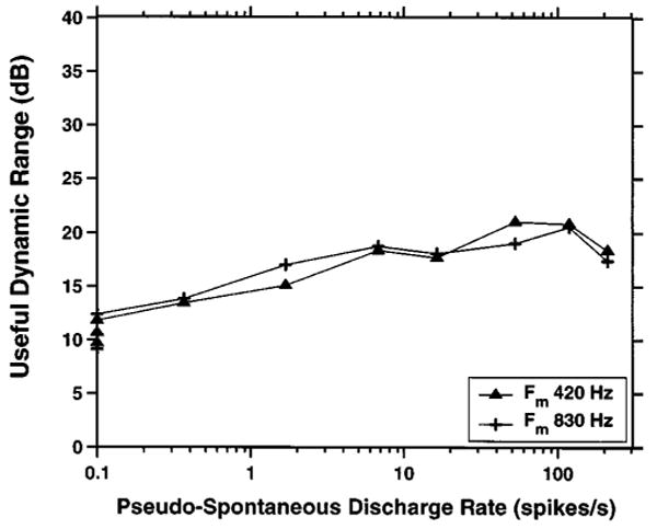
Figure 11 shows the useful dynamic range as a function of pseudo-spontaneous discharge rate for the 417- and 833-Hz modulators. Regression lines were fit to the dynamic range at each frequency against the logarithm of the pseudo-spontaneous rate (Table II). The slopes of the regression lines were constrained to be the same at both frequencies because a regression with separate slopes did not significantly reduce the mean square error (p = 0.21). The slope of the regression line is 2.3 dB/decade, meaning that a tenfold increase in pseudo-spontaneous rate increases the dynamic range by 2.3 dB. The statistical significance of this trend is confirmed by the entirely positive 95% confidence intervals for the slope in Table II.

FIG. 11.

Useful dynamic range to sinusoidal modulations of a DPT as a function of pseudo-spontaneous rate for modulation frequencies of 417 and 833 Hz. The useful dynamic range is the ratio of the modulation depth that evokes a discharge rate of 300 spikes/s to the synchronized rate threshold. Each point shows data from one fiber. Symbols code modulation frequencies. The straight lines are least-squares fits to the data for each frequency, with the constraint that the slopes be the same for both frequencies (see Table II).

TABLE II.

Dependence of useful dynamic range on pseudo-spontaneous rate (PSR) and modulation frequency (F_m). The dynamic range DR in dB was fit by the equation DR = A + B log₁₀(PSR). The table shows means and 95% confidence intervals for the slope B and the value of the fitted line at 50 spikes/s. Confidence intervals are based on 5000 bootstrap replications of the regression line (Efron and Tibshirani, 1993, Chap. 7). The slopes of the regression lines were constrained to be the same at both modulation frequencies because a model with separate slopes did not significantly improve the fit.

Fm (Hz)	Slope (dB/decade)		Dynamic range at 50 spikes/s (dB)
	Mean	95% C.I.	Mean	95% C.I.
417	2.32	1.21–3.43	22.7	20.9–24.6
833	same	same	18.3	16.7–19.9

The average useful dynamic range of sustained responders is 23 dB for the 417-Hz modulator, and 17 dB for the 833-Hz modulator. The difference between the two means is highly significant (p<0.001, two-sided permutation test for difference in means). These values of dynamic range are comparable to those observed with pure-tone stimulation in a normal ear (Sachs and Abbas, 1974), and considerably larger than the dynamic ranges observed with sinusoidal electric stimulation without a DPT (van den Honert and Stypulkovsky, 1987; Hartmann et al., 1990; Dynes and Delgutte, 1992). In contrast, transient DPT responders have useful dynamic ranges as low as 10 dB, more in line with electric dynamic ranges reported in the literature. However, Fig. 11 may not give a completely representative picture of the dynamic range of transient responders because it does not include data from the fibers (primarily transient responders) whose discharge rates failed to reach the 300 spikes/s upper limit of the useful dynamic range at the highest modulation depth tested.

While the DPT-induced increase in dynamic range for sustained responders is encouraging, a key question is what fraction of the population of auditory-nerve fibers would be likely to benefit from a DPT at a given level. To address this question, solid lines in Fig. 12 shows the percentage of fibers that gave “acoustic-like” responses to the 417- and 833-Hz sinusoidal modulators as a function of modulation depth. By “acousticlike,” we mean that the response is above the synchronized rate threshold and the average rate is below 300 spikes/s. Percentages are computed separately for sustained and transient DPT responders. Dotted curves indicate the percentage of fibers that have sustained discharge rates above 300 spikes/s, and are therefore above the normal acoustic range. For modulation depths between 1% and 5%, most sustained responders have responses within the acoustic range at both frequencies. For modulation depths of 10% and above, most sustained DPT responders have discharge rates above the normal acoustic range. On the other hand, modulation depth has to exceed 5% for a majority of transient DPT responders to respond to the modulation. Because approximately 50% of the fibers in our entire sample from ten animals were transient responders (Litvak et al., 2003b), the percentage of acoustic-like responses for this sample (not shown) would be nearly the mean of that for the sustained and transient responders. Overall, a substantial fraction (40%–55%) of the fibers would exhibit acoustic-like responses for modulation depths between 1% and 5%. Of course, these estimates are likely depend on the choice of DPT amplitude.

FIG. 12.

This figure shows, as a function of modulation depth, the percentage of fibers whose responses to a modulated DPT are within the useful dynamic range (solid lines), as well as the percentage of fibers that exceed the maximal acoustic rate of 300 spikes/s (dashed lines) for modulation frequencies of 417 Hz (left) and 833 Hz (right). Percentages are shown separately for sustained and transient DPT responders. Only responses that were recorded at the standard DPT level in each animal (Table I in Litvak et al., 2003b) are included.

E. Responses of the stochastic threshold model

Several key features of ANF responses to sinusoidally modulated DPTs are predicted by an extremely simple stochastic threshold model (STM). The STM produces a spike whenever the modulation waveform m(t) crosses a noisy threshold (Fig. 2). The response of the model is entirely determined by two dimensionless parameters: m/σ and θ₀/σ. The input-to-noise ratio m/σ determines the effective stimulus level (modulation depth), while the threshold-to-noise ratio θ₀/σ determines the pseudo-spontaneous discharge rate in the absence of modulation. We will show that the relationship between the STM's pseudo-spontaneous rate and its responses to sinusoidal modulators is similar to that seen in the data.

Figure 13 shows the average discharge rate and synchronization index as a function of m/σ for model fibers with different pseudo-spontaneous discharge rates (different values of θ₀/σ). The model predicts several features of the data shown in Fig. 9: (1) Both average rate and synchrony grow over a wide range of modulation depths. (2) Both model and neural fibers with low (<5 spikes/s) pseudo-spontaneous rates have higher modulation thresholds than fibers with high pseudo-spontaneous rates. (3) For both model and neural fibers with high pseudo-spontaneous rates, synchrony grows rapidly at low modulation depths, while the average rate remains near pseudo-spontaneous. In contrast, fibers with low pseudo-spontaneous rates show high synchrony as soon as the modulation depth reaches threshold. (4) For both model and data, synchrony grows nonmonotonically with modulation depth at 104 Hz due to the occurrence of multiple spikes in each stimulus cycle at high levels. However, the maximum discharge rates exhibited by the model are larger than those seen in the data. In addition, while neural synchrony grows monotonically with modulation depth at 417 Hz, synchrony is somewhat nonmonotonic in the model responses at very high discharge rates.

FIG. 13.

Average discharge rate (left) and synchronization index (right) of the stochastic threshold model as a function of the normalized modulation depth m/σ for three modulations frequencies (rows). Each curve corresponds to one value of the threshold to noise ratio θ₀/σ: 1.4 (dot-dash), 1.8 (dash), 2.4 (dot), and 4 (solid). The corresponding pseudo-spontaneous discharge rates are 210, 119, 30, and 0.2 spikes/s, respectively.

Figure 14 shows the model average and synchronized rate thresholds as a function of pseudo-spontaneous rate for three modulation frequencies. These predictions can be directly compared to the neural thresholds in Fig. 10. Note, however, that while the neural pseudo-spontaneous discharge rates are always below 200 spikes/s, the model rates were extended to 600 spikes/s. For both model and data, average rate thresholds decrease nearly linearly with the logarithm of pseudo-spontaneous rate at relatively low rates for all three modulation frequencies. The model thresholds behave nonmonotonically, increasing steeply once the pseudo-spontaneous rate exceeds the modulation frequency. Such nonmonotonic dependence of detectability on noise amplitude (which controls the pseudo-spontaneous rate) is a defining characteristic of stochastic resonance (Wiesenfeld and Moss, 1995). Some evidence for a nonmonotonicity can also be discerned in the neural data of Fig. 10 for the 104-Hz modulator in that thresholds for pseudo-spontaneous rates above 40 spikes/s lie above the regression line fit to the data at lower pseudo-spontaneous rates. However, the data show no nonmonotonicity at 417 and 833 Hz, presumably because the pseudo-spontaneous rates always remain well below the modulation frequency.

FIG. 14.

Normalized modulation depth thresholds m/σ based on average rate (left) and synchronized rate (right) as a function of pseudo-spontaneous rate for the stochastic threshold model. Symbols code modulation frequencies.

The model synchronized rate thresholds decrease nearly linearly with the logarithm of pseudo-spontaneous rate for all three modulation frequencies. The synchronized rate thresholds decrease more rapidly than the average rate thresholds. The same trends are apparent in the data for the 417-Hz modulator (Fig. 10). However, only the data show a dependence of thresholds on modulation frequency, with the lowest thresholds at 417 Hz.

Figure 15 shows the model useful dynamic range as a function of pseudo-spontaneous rate for 417- and 833-Hz modulators. As for the data, the useful dynamic range is the ratio of the modulation depth that evokes a discharge rate of 300 spikes/s to the synchronized rate threshold. Because the dynamic range is a ratio of modulation depths, there are no free parameters in this plot. The model dynamic range increases linearly with the logarithm of pseudo-spontaneous rate up to 50 spikes/s, then flattens out at about 19 dB for both frequencies. The increase in dynamic range at low pseudo-spontaneous rates is apparent in the data of Fig. 11, but the plateau at high rates is less obvious. The model's plateau dynamic range (19 dB) is intermediate between the mean 23-dB dynamic range in the data for the 417-Hz modulator and the 17 dB observed for the 833-Hz modulator. However, the model does not predict the difference in dynamic ranges between the two modulation frequencies.

FIG. 15.

Useful dynamic range of the stochastic threshold model as a function of pseudo-spontaneous rate for two modulation frequencies. The definition of useful dynamic range is the same as in Fig. 11.

Overall, the stochastic threshold model does a good job of predicting the relationship between the pseudo-spontaneous discharge rates of ANFs and their responses to sinusoidal modulators at a given frequency. However, this version of the model cannot account for the frequency dependence of neural sensitivity to modulation.

IV. Discussion

A. Representation of sinusoid in temporal discharge patterns

All auditory-nerve fibers in our study responded to sinusoidal modulations of the DPT. Neurons that had sustained responses to the DPT were the most sensitive to modulations. These neurons showed strong phase locking to the modulator for modulation depths as low as 0.5%. In these neurons, the average discharge rate grew monotonically with modulation depth over a range of 17–23 dB before reaching 300 spikes/s, the upper limit of discharge rates for pure-tone stimulation. The temporal discharge patterns to modulation depths below 2.5%–5% resembled acoustic responses to pure tones. These responses were stochastic, with interspike intervals occurring at random at multiples of the modulator period. The period histograms of these responses were similar to those seen in responses to pure tones, and provided a good representation of the sinusoidal stimulus waveform.

For modulation depths above 5%–10%, sustained DPT responders exhibited higher discharge rates than those seen for acoustic stimulation. For 417-Hz modulation, discharges tended to entrain (occur once per stimulus cycle) while, for 833-Hz modulation, some neurons fired exactly on every other stimulus cycle. These responses were more precisely phase locked than acoustic responses. In most respects, responses to large modulations of the DPT resemble suprathreshold responses to sinusoidal electric stimulation without a DPT (Hartmann et al., 1984; van den Honert and Stypulkowski, 1987).

Fibers that only responded transiently to the unmodulated DPT nevertheless responded with phase-locked spike discharges to sinusoidal modulations. However, larger modulation depths were needed to produce a response in these fibers than in sustained responders. Thus, the introduction of a DPT qualitatively mimics the threshold differences between high-spontaneous and low-spontaneous fibers observed in normal ears (Liberman, 1978). At these large modulation depths, the responses of transient DPT responders were more synchronized than responses to tones in a normal ear, and poorly represented the stimulus waveform. In addition, transient DPT responders had a smaller dynamic range than sustained responders. In this respect, transient responders differ from low spontaneous-rate ANFs in a healthy ear, which have wider dynamic ranges than high spontaneous fibers (Schalk and Sachs, 1980).

The deafening protocol in these experiments was only partly successful in that some animals had residual hearing in the nonimplanted ear (Litvak et al., 2003b). This observation raises the possibility that the acoustic-like responses of sustained responders may reflect hair-cell mediated activity. Although we cannot rule out this possibility in every case, we did observe acoustic-like responses to modulations of the DPT in animals with no residual hearing as well as in animals with substantial hearing. Our measure of residual hearing was very conservative in that it did not take into account any additional hearing loss caused by insertion of the stimulating electrodes into the implanted cochlea.

While the temporal discharge patterns of sustained responders to small sinusoidal modulations of a DPT resemble responses to pure tones in a healthy ear, there are nevertheless differences in the interspike interval distributions between the two modes of stimulation. While the interspike distributions in response to a pure tone always show a mode at the tone period for frequencies below 1 kHz, this mode was often lacking in responses to 417-Hz electric modulations. This lack of a mode at the stimulus period has also been observed for 500-Hz sinusoidal electric stimulation without a DPT (van de Honert and Stypulkowski, 1987). In addition, for neurons having nonexponential interspike interval distributions in responses to unmodulated DPTs, modes in the interval histogram for sinusoidal modulators were often systematically shifted away from multiples of the stimulus period, particularly for very low modulation depths. These shifts are considerably larger than the small, but systematic offsets seen in interspike interval distributions to pure tones in a healthy ear (McKinney and Delgutte, 1999). The mode offsets seen with modulated DPTs seem to reflect an interaction between the stimulus period and the intrinsic dynamics of the neural membrane leading to preferred intervals in response to the unmodulated DPT. Preferred intervals have also been noted for electric stimulation with high-frequency (>1 kHz) sinusoids without a DPT, and found to distort phase locking to the stimulus (Parkins, 1989).

Although interspike interval distributions of sustained DPT responders for small sinusoidal modulations differ somewhat from responses to pure tones in a healthy ear, these distortions may not severely interfere with neural representation of the stimulus frequency. Because there is no evidence for cross-fiber correlation in responses to unmodulated DPTs (Litvak et al., 2003b), responses to small modulations of a DPT may be conditionally uncorrelated from one fiber to the next. By “conditionally uncorrelated,” we mean that the occurrence of a spike on a particular stimulus cycle for one fiber does not alter the probability that a spike occurs on the same cycle in another fiber. By integrating synaptic inputs from several conditionally uncorrelated auditory-nerve fibers, some central auditory neurons might show a mode at the stimulus period in their interval histograms even if such a mode is lacking in their ANF inputs. Similarly because mode offsets in interspike intervals differ from one fiber to the next and can be either positive or negative (Fig. 8), these offsets might average out in the responses of integrating central neurons so as to produce a mode centered at the stimulus period. Nevertheless, both distortions could degrade somewhat the accuracy of frequency representation. Direct recordings from central neurons (e.g., cochlear nucleus) in response to a modulated DPT stimulus would test whether synaptic integration suffices to overcome the distortions in the coding of the modulation frequency observed in the auditory nerve.

B. Dynamic range

A major finding of the present study is the relatively wide dynamic range (17–23 dB) for sustained DPT responders. In studies of electric stimulation, dynamic range is normally measured by the varying the amplitude of a stimulus without changing its waveform, and determining the range of amplitudes over which the discharge rate changes. Here, we varied the depth of sinusoidal modulations of a DPT, and determined the range of modulation depths over which either average rate or synchronized rate varied (with an upper limit of 300 spikes/s for average rate). As shown in Fig. 1, this method is equivalent to varying the amplitude of a 100%-modulated stimulus superimposed upon a fixed, unmodulated DPT, which is not considered part of the information-bearing stimulus since its function is to evoke pseudo-spontaneous activity. Because modulation depth in percent can be translated into stimulus amplitude in mA by simple multiplication by the DPT amplitude in mA, a modulation-depth dynamic range in dB is numerically equivalent to a conventional dynamic range for the information-bearing part of the stimulus (excluding the fixed DPT).

The most detailed information on dynamic range for electric stimulation comes from the example of rate-level functions for periodic trains of biphasic pulses shown by Javel and his colleagues (Javel et al., 1987; Javel, 1990; Shepherd and Javel, 1997; Javel and Shepherd, 2000). Although no formal statistics are provided, the dynamic ranges for the highest pulse rate tested (800 pps) range from 3 to 12 dB in the examples shown, with a median near 6 dB. The discharge rates of the fibers studied by Javel et al. typically approached the 800/s pulse rate at high stimulus amplitudes. Therefore, the dynamic ranges would only be about half as large if a 300 spikes/s upper limit was imposed, as we did in the present study. These values are consistent with those reported for sinusoidal electric stimulation at frequencies of 1 kHz and above (van den Honert and Stypulkowski, 1987; Hartmann et al., 1990; Dynes and Delgutte, 1992). They are also consistent with the 2–4 dB conventional dynamic ranges measured in our earlier study (Litvak et al., 2001) for 4.8-kpps pulse trains sinusoidally modulated at 400 Hz with a 10% depth. The modulation dynamic ranges observed for transient DPT responders (as low as 10 dB) overlap with the values given in the literature for sinusoidal or pulsatile stimuli. However, the 17–23 dB dynamic ranges of sustained DPT responders are clearly higher than any of the values reported in the literature.

The improvement in dynamic range resulting from the introduction of a DPT in sustained responders arises from at least two distinct effects. First, the pseudo-spontaneous activity evoked by the DPT allows synchronized rate thresholds to be about 10 dB lower than the average rate thresholds. In this range of modulation depths, the stimulus sinusoidally modulates the pseudo-spontaneous activity without causing an increase in average rate, as is the case in a spontaneously active fiber with acoustic stimulation.

The second effect giving rise to improved dynamic range with a DPT is that, because rate-level functions are expansive near threshold, the response to the superposition of two stimuli is always greater than the sum of the responses to each of the stimuli. The presence of a DPT therefore allows the superimposed modulated stimulus to evoke an increment in discharge rate over background, even if, by itself, this stimulus would be below threshold. Because rate-level functions become compressive rather than expansive near their saturation, this mechanism is likely to be effective over only a limited range of pseudo-spontaneous rates. Specifically, if the pseudo-spontaneous rate approached the upper limit imposed by neural refractoriness, the threshold for superimposed stimuli would be expected to increase rather than decrease. Such an increase in rate thresholds is observed for the stochastic threshold model at high pseudo-spontaneous rates (Fig. 14). However, this condition did not occur in our data (Fig. 10), presumably because pronounced adaptation over the course of the DPT always kept the pseudo-spontaneous rates well below saturation (Litvak et al., 2003b). Adaptation to the continuous DPT is thus likely to play an indirect role in improving the dynamic range. Whether it also plays a more direct role, for example by decreasing the slopes of rate-level functions, cannot be determined from our data.

The above reasoning suggests that the effectiveness of a DPT in lowering threshold and increasing dynamic range does not depend on either the exact parameters of the DPT, or the particular scheme used for encoding the sinusoidal stimulus, so long as the pseudo-spontaneous rate evoked by the DPT lies in the appropriate range. Thus, a DPT might remain effective if an analog sinusoidal stimulus was simply added to the DPT, as originally proposed by Rubinstein et al. (1999b), rather than encoded as a modulation of the DPT. In other words, a DPT may be as effective with an analog stimulation strategy as with the CIS-type strategy used in this paper. Similarly, a lower-rate pulse train (e.g., 1 kpps) might be equally effective as our 5-kpps DPT in improving the dynamic range. However, since ANFs adapt less to low-rate pulse trains than to high-rate trains (Moxon, 1967; van den Honert and Stypulkowski, 1987), more fibers might be near saturation of the input–output function with a low-rate DPT. A low-rate DPT would have the further disadvantage that phase locking to the pulse rate might give rise to pitch sensations that would bear no relation to the sinusoidal stimulus. In addition, if sinusoidal stimuli are encoded as modulations of the DPT, the low rate of a 1-kpps pulse train would prevent all but very low frequency signals to be encoded without aliasing the modulation waveform. Thus, a 5-kpps DPT seems to be preferable over a lower-rate DPT, particularly with a CIS-type strategy.

C. Comparison with models of electrically stimulated fibers

1. The stochastic threshold model

We presented a stochastic threshold model of ANF responses to modulations of a DPT. Despite its simplicity, the STM accounts for the dependence of both threshold and dynamic range on the pseudo-spontaneous discharge rate evoked by the unmodulated DPT. In addition, the STM quantitatively predicts (within 2–4 dB) the average useful dynamic range of sustained DPT responders. However, the dependence of threshold and dynamic range on modulation frequency is not predicted by the STM. A parsimonious way to account for that dependence would be to introduce a bandpass filter at the input to the model, so as to amplify modulation frequencies near 400 Hz. We show in a companion paper (Litvak et al., 2003a) that such a filter is also necessary to account for ANF responses to complex modulations of a DPT.

It may seem at first sight surprising that the dependence of threshold and dynamic range on pseudo-spontaneous rate is predicted by the very simple stochastic threshold model. We believe that the agreement is not accidental. Many bio-physically realistic neural models can be approximated by a driving function, which depends only on the stimulus, and another (possibly noisy) function describing threshold dynamics, which depends only on previous activity (e.g., Hill, 1936). In general, the driving function may depend on the stimulus in a complex, nonlinear way. However, because the stimuli in our study are composed of a large signal (the DPT) perturbed by small modulators, the driving function may be linearized around the operating point imposed by the DPT. Thus, to the extent that the threshold component of the model captures the complex dynamics of neural refractoriness, the stochastic threshold model can be considered an approximation of a more realistic neural model for small modulation depths.

It is worth emphasizing that the DPT is not explicitly represented in the STM because the input to the model is the modulation waveform without a pulse-train carrier. The effect of a DPT is simulated in the model by varying the threshold-to-noise ratio θ₀/σ (Fig. 2), which controls the pseudo-spontaneous rate. The pseudo-spontaneous rate can be increased by either decreasing the resting threshold θ₀ or, equivalently, increasing the neural noise. That the STM can nevertheless predict the effects of a DPT on neural responses to modulations bolsters the argument made in the previous section that the effectiveness of a DPT in improving dynamic range and temporal discharge patterns is not likely to depend on the exact characteristics of the DPT such as its pulse rate.

2. The Rubinstein biophysical model

In many respects, ANF responses to a modulated DPT also resemble the responses of a biophysical model to electric sinusoids in the presence of a 5-kpps conditioner (Rubinstein et al., 1998). At low levels of the electric sinusoid, period histograms for this model resemble the sinusoidal stimulus waveform. We obtained a similar result for responses to small modulations of the DPT. The useful dynamic range of the biophysical model responses was near 20 dB, and changed little with DPT level, so long as the DPT evoked discharge rates between 10 and 250 spikes/s. The measured responses to the modulated DPT showed a similar trend, with no systematic relationship between the pseudo-spontaneous rate and useful dynamic range for discharge rates above 5 spikes/s (Fig. 11). Because Rubinstein et al. did not report interval histograms of model responses to the sinusoid, it is unclear whether their model captures the mode shifts, and the missing first mode observed in the data. Although responses of the biophysical model of Rubinstein et al. (1999b) to a modulated DPT remain to be studied in detail, the results so far suggest that this model captures the essential features of responses of ANFs to sinusoidal electric stimulation.

D. Function of spontaneous activity

Spontaneous activity in sensory neurons is often considered as noise that imposes fundamental limitations on the performance achievable by an ideal observer in any detection or discrimination task based on the neural discharge patterns (Barlow and Levick, 1969; Siebert, 1965; Werner and Mountcastle, 1965). While this point of view is certainly valid, it does not specify a functional advantage of spontaneous activity that might account for its nearly ubiquitous presence in primary sensory neurons (Retinal ganglion cells: Kuffler, 1953; Rodieck, 1967; Somatosensory afferents: Werner and Mountcastle, 1965; Auditory nerve: Kiang et al., 1965; Vestibular nerve: Goldberg and Fernandez, 1971; Walsh et al., 1972; Olfactory receptors: Chaput and Holley, 1979; Rosparset et al., 1994; Gustatory receptors: Pfaffmann, 1955). Our physiological and modeling results, as well as those of others (Yu and Lewis, 1989; Schneidman et al., 1998; Rubinstein et al., 1999a, b) suggest such an advantage.

Spontaneous activity helps to faithfully encode stimulus waveforms in the temporal discharge patterns of sensory neurons by allowing these waveforms to be represented by small modulations of ongoing activity. Such modulation coding lowers threshold and mitigates the distortions caused by refractoriness in single neurons. Spontaneous activity may also desynchronize stimulus-driven activity across neurons in a population, thereby allowing a volley principle to operate when the stimulus period is shorter than the neural refractory period. In this view, noise resulting from random spontaneous activity is the price paid for the lower thresholds and improved temporal representation of waveforms in the neural population. The performance limitations imposed by noise can, in principle, be reduced by averaging responses across similarly driven neurons. The net result will be beneficial if the population is large enough and the noise largely uncorrelated across neurons.

E. Comparison with psychophysical modulation detection thresholds

It is of interest to compare our single-fiber modulation detection thresholds with psychophysical thresholds for human cochlear implant listeners (Shannon, 1992). In that study, subjects were stimulated continuously with 500–2000-Hz sinusoids. Beats were produced by presenting another sinusoid differing slightly in frequency. Because our neural threshold criterion closely parallels that used in psychophysics, direct comparison of threshold values is appropriate.

Shannon found that subjects were most sensitive to 100-Hz beats. At these frequencies, a modulation depth of 1% could be detected. These modulation depths are comparable to the most sensitive rate modulation detection thresholds that we observed for 104-Hz modulators, and are close to the mean synchronized rate thresholds. Unlike the neural data, however, sensitivity of human subjects to beats dropped rapidly with increasing beat frequency. The best psychophysical modulation detection thresholds for a 400-Hz modulator were near 3%. In contrast, our rate-based neural detection thresholds were lower for 417- than for 104-Hz modulation, and could be as low as 0.4%.

Shannon (1992) suggested that the drop in the subjects' ability to detect modulations with increasing beat frequency may reflect a central limitation in sensitivity to high-frequency modulations. Because the peripheral neurons encode 400-Hz modulations at least as well as 100-Hz modulations, our data are consistent with this view. However, the differences between our neural data and Shannon's (1992) psychophysical thresholds might also be accounted for by differences in stimuli (sinusoidal modulations of a 5-kpps pulse train versus beats of a 0.5–2 kHz sinusoid). Psychophysical studies with stimuli more similar to those used in this study are needed to determine how well higher-frequency modulations of a DPT can be detected by human listeners.

F. Implications for cochlear implant processors

Our results strongly suggest that a high-rate, ongoing DPT can enhance the representation of the temporal fine structure of sinusoids in auditory nerve responses for frequencies up to at least 800 Hz. The enhancement is maximal for small (<5%) modulations of the DPT and is most apparent in fibers that have sustained responses to the DPT. Specifically, responses of sustained DPT responders to small modulations resemble responses to sound in a healthy ear in at least four respects: (1) the dynamic range is near 20 dB; (2) interspike intervals occur randomly at multiples of the stimulus period; (3) spikes are distributed over most of one-half cycle, thereby giving a faithful representation of the stimulus waveform; and (4) there is a range of stimulus levels over which synchrony grows rapidly with little or no increase in average rate. No other strategy for electric stimulation has been shown to exhibit any of these properties over a wide range of levels and frequencies. These observations suggest that a processing strategy that incorporates a DPT, and that preserves temporal fine structure information in the signals delivered to the stimulating electrodes, may improve performance of cochlear implant users. In particular, improved coding of the sound fine-time structure may lead to improved perception of musical pitch, and to more effective utilization of binaural cues in bilateral implants (Smith et al., 2002).

One stimulation strategy that does preserve the fine-time structure of the signals delivered to the stimulating electrodes is the continuous analog (CA) strategy. Because a DPT may allow for better encoding of the fine-time structure, performance with a CA strategy may be substantially enhanced by a DPT. In current implementations, the CIS strategy discards the fine-time structure at the envelope detector stage. One function of the envelope detector is to produce a strictly positive modulation waveform that can be used to modulate a carrier pulse train. Because negative waveforms can be represented as decreases in DPT amplitude, it may be possible to entirely eliminate the envelope detector stage in DPT-enhanced CIS strategies. The rate of the pulse-train carrier would also have to be increased in order to sample the higher modulation frequencies without aliasing. Thus, a DPT may be beneficial with CIS as well as with CA strategies, so long that the information-bearing signals are small compared to the ongoing DPT.

We found that sustained DPT responders are best at representing the sinusoidal stimuli in their temporal discharge patterns. A comfortable majority of the sustained responders in our data gave acousticlike responses for modulation depths below 5% (Fig. 12). A key question is what fraction of the auditory-nerve population has a sustained response to a given DPT level. In the companion paper (Litvak et al., 2003b), we showed that the DPT needs to be at least 4 dB above ECAP threshold to evoke a sustained response in a sizeable fraction of the neurons, but that DPT levels more than 8 dB above ECAP threshold can evoke long-lasting changes in neural excitability, and may therefore be harmful to the nerve. To stimulate a large number of fibers, while simultaneously meeting the safety constraint, it may be advantageous to present a DPT at a low (4 dB above ECAP threshold) level on several electrodes. Further research is needed to work out the best trade-off between the safety of DPT stimulation and its effectiveness.

The transient responders comprised roughly 50% of the neurons that we recorded from in our sample from ten ani-nals. Even though a strategy that uses only small modulation depths may stimulate only half of the neurons that are excited electrically, it may still produce substantial benefit by mimicking some aspects of normal ANF responses in the neurons that it does stimulate. On the other hand, even with a large number of fibers showing fairly natural temporal discharge patterns, the central nervous system might not be able to make use of this information if temporal processing depends critically on factors that were not considered here such as phase relationships between response of fibers innervating different locations (Heinz et al., 2001; Shamma and Klein, 2000).

Our results suggest that a DPT would decrease thresholds to electric stimulation. In the case of CIS, if the CIS carrier and the DPT are in phase, then our results suggest that there would be sufficient information in the auditory nerve to detect modulations as small as 0.5% for 417-Hz modulators, and near 1 to 2% for 104- and 833-Hz modulators. For a DPT level of 2 mA and a modulation depth of 0.5%, the amplitude of the modulation waveform is only 10 μA, which is considerably lower than typical single-unit thresholds reported for sinusoidal electric stimulation. While these results are promising, the improvements in single-fiber thresholds may not necessarily translate into improvements in psychophysical dynamic range because the latter is determined by the distribution of ANF thresholds as well as by the dynamic range of individual fibers. Because a DPT is expected to modify the threshold distribution, its effect on the psychophysical dynamic range is unclear.

V. General Conclusion

We showed that, using a DPT, it may be possible to design strategies for cochlear implants that would realistically code the fine-time structure of sound stimuli in the temporal discharge patterns of electrically stimulated auditory-nerve fibers. If the central nervous system can make use of this information, then these strategies may substantially improve the quality of auditory experience enjoyed by cochlear implant users.

Appendix A: Method for Artifact Rejection

Single-unit recordings in response to electric stimulation are contaminated by two distinct signals with can interfere with detection of action potentials: (1) the stimulus artifact proper, representing the voltage drop between the recording electrodes directly due to the stimulating current, and (2) evoked potentials reflecting the summed activity of many neurons recorded in the far field. For convenience, we refer to the superposition of these interfering signals as “the artifact.”

To remove the artifact from responses off-line, we first filtered the recorded signal using a moving average filter of length equal to the carrier period (0.2 ms). This filter removed the 5-kpps periodic component from the artifact. For modulation depths below 2.5%, the remaining artifact was smaller than the noise in the recording for nearly all of the records. For modulation depths between 2.5% and 15%, however, the artifact was often comparable in amplitude to the spikes. The top row of Fig. 16 shows a typical waveform and spectrum of the recorded signal after processing by the moving-average filter. This signal, which we denote by y(t), is the sum of (1) the artifact waveform a(t), (2) the spike train x(t), and (3) noise n(t). In this example, the modulator frequency is 417 Hz. As expected, the spectrum has its largest peaks at the two components present in the stimulus: 5000−417 Hz and 5000+417 Hz. In addition, there are peaks at the 417-Hz modulation frequency and its harmonics 834 and 1251 Hz. These peaks are distortion products of the modulator waveform, and indicate the nonlinear nature of the artifact (including evoked responses). While the higher-frequency components at 5000±417 Hz can easily be removed by low-pass filtering (Fig. 16, second row), the low-frequency distortion products occur in the region where spikes have significant energy, and therefore cannot be simply filtered out.

FIG. 16.

Algorithm for removing the stimulus artifact from contaminated recordings. The top row shows the waveform (left) and the spectrum (right) of the signal recorded from a microelectrode after it has been passed through a 0.2-ms moving-average filter. The stimulus is a sinusoidally modulated pulse train (modulation frequency: 417 Hz; modulation depth: 5%). The inset shows the spike waveform for an unmodulated pulse train. The middle row shows the waveform and spectrum after low-pass filtering the signal at 3 kHz. The bottom row shows the waveform and spectrum after eight steps of the iterative artifact rejection algorithm described in Appendix A.

We developed an iterative algorithm to remove these low-frequency components of the artifact. The algorithm is based on two assumptions: (1) that the artifact a(t) can be represented by a low-order Fourier series of the modulator frequency, and (2) that the spike train x(t) is composed of spikes whose waveform is known within an overall gain. The principle of the algorithm is to refine an estimate of a(t) until the spikes in the estimated neural response y(t) − a(t) maximally resemble spikes recorded during the unmodulated DPT (Fig. 16, upper left panel, inset). While the artifact is always a low-order Fourier series, the spikes, which have rapid rise times and occur with some jitter relative to the modulator, are poorly represented by this Fourier series. Thus, it is unlikely that spikes would be erroneously introduced or removed by this algorithm.

As an initial guess a⁰(t) for the artifact waveform, we use the first three Fourier components of the minimum of the recorded signal y(t) over all modulator periods. The rationale is that, because spikes are mostly positive, y(t) is likely to have smaller amplitude during a modulation cycle which contains no spikes than during cycles in which a spike does occur. Nevertheless, the algorithm works even if spikes occur on every cycle, so long as they show sufficient time jitter.

At step n, the algorithm first estimates the noisy neural response xⁿ(t) using the equation xⁿ(t)=y(t)−aⁿ⁻¹(t), where aⁿ⁻¹(t) is the artifact estimate at step n−1. Next, this noisy response is fit by a model neural response ${\widehat{x}}^n(t)$, which is defined as

$${\widehat{x}}^n(t)=\sum _j{g}_j\hspace{0.17em}·\hspace{0.17em}s(t-{\tau }_j),$$ (A1)

where j is spike number, s(t) is the known spike waveform, while g_j and τ_j are the spike gains and spike times, respectively. The g_j's and τ_j's are determined by cross-correlating xⁿ(t) with the spike waveform s(t). Spikes are assumed to occur whenever the correlation coefficient is larger than a threshold, which was normally set at 20%, but was increased for particularly noisy recordings. Whenever a spike is detected, its gain g_j is determined from the local maximum of the correlation, while the location of the maximum is taken as spike time τ_j. Finally, the artifact waveform aⁿ(t) at step n is estimated from the first three Fourier components of $y(t)-{\widehat{x}}^n(t)$.

The algorithm is stopped whenever the difference between aⁿ(t) and aⁿ⁻¹(t) is less than 0.1% of the spike height. The bottom row of Fig. 16 shows the estimated neural response x(t) after eight iterations. The dotted line is the estimated artifact a(t). In this case, the estimated spikes match those that would be picked by an experienced eye.

The algorithm was tested using synthetic neural recordings in response to 100-, 400-, and 800-Hz modulators. The synthetic recordings were composed of stereotyped spikes similar to those recorded from ANFs, and additive white noise.³ For the 100- and 400-Hz stimuli, one synthetic spike occurred on every stimulus cycle with uniformly distributed time jitter. For 800 Hz, a spike occurred on every other cycle. Time jitter and noise amplitude were systematically varied from 50 to 400 μs and from 0% to 30% of spike amplitude, respectively. The algorithm was applied to synthetic spike trains comprising responses to 25 response cycles. For each noise and jitter condition, the procedure was repeated 100 times, and the maximum deviation between the estimated and the actual artifact waveforms was computed. For all conditions, this deviation was less than 10% of spike height. The largest deviations were seen for responses to the 800-Hz modulator.

The results of the algorithm were also monitored for real neural recordings, and a record was rejected if the estimated neural signal did not resemble spikes. This occurred in only about 2% of the records and only at the largest modulation depths.

Appendix B: Method for Estimating Modulation Threshold

Single-fiber modulation threshold was defined in this study as the modulation depth at which either the average discharge rate or the synchronized rate during the sinusoidal modulation exceeded the discharge rate during a following unmodulated DPT segment on 75% of stimulus trials. The most direct method to determine threshold would rely on the percentage of hit trials, those in which the rate during the modulation exceeds the rate during the unmodulated DPT. To reliably estimate threshold by this method, the data would need to span the 75% criterion over the range of modulation depths tested. This condition was rarely met, particularly when measuring the very low synchronized rate thresholds for a 417-Hz modulator. A common pattern in the data was a hit percentage between 75% and 95% for the smallest measured modulation depth, and 100% for all larger modulation depths. Examples of this pattern are shown for three of the four fibers in the left panel of Fig. 17. In such cases, it is not possible to reliably fit a curve to the data so as to extrapolate the hit percentage to the 75% threshold criterion.

FIG. 17.

Method for estimating modulation depth thresholds. The left panel shows the percentage of hit trials against depth of modulation at 417 Hz for four sustained DPT responders. For three of these fibers, the hit percentage was below 100% for only one modulation depth, preventing a direct determination of threshold. The middle panel plots the quartile rate difference ${\text{r}}_d^q(m)$ against modulation depth for the same four fibers. The dotted line indicates the threshold criterion. The right panel shows the same data plotted on an inverted Gaussian vertical scale defined by Eq. (B2). Gray shading indicates the region where the data grow approximately linearly. Circled symbols show the estimated thresholds.

We therefore developed an alternative method for determining threshold which does not directly depend on hit percentages. The method seeks to utilize data points for which the hit percentage is 100%. To this end, we developed a measure, called quartile rate difference, which continues to grow with modulation depth even when the hit percentage reaches 100%. For each modulation depth m, and each trial i, let r_m(m,i) denote the rate during the modulation (rate can be either synchronized or average discharge rate), and let r_u(m,i) denote the rate during the corresponding unmodulated segment. The quantity r_d(m,i) = r_m(m,i)−r_u(m,i) is the rate difference. The quartile rate difference ${\text{r}}_d^q(m)$ is the 25th percentile of r_d(m,i) over all stimulus trials (modulated segments). By definition, at modulation threshold, the rate difference is positive on 75% of the trials (i.e., the rate during the modulation exceeds the rate during the corresponding unmodulated segment), and negative on the other 25% of the trials, so ${\text{r}}_d^q(m)$ must be zero. Thus, to determine threshold, we need to find the modulation depth m_thr such that ${\text{r}}_d^q(m_{\text{thr}})=0$.⁴

The middle panel of Fig. 17 shows the quartile rate difference as a function of modulation depth for the same data set as in the left panel. The threshold criterion of 0 is shown as a dotted line. Theoretically, as m approaches 0, ${\text{r}}_d^q(m)$ approaches a negative value r₀, which is the 25% percentile of r_u(m,i)−r_u(m,j) for all pairs of trials (i,j). This value was estimated directly from responses to the unmodulated DPT segments. For 55% of the synchronized rate records, ${\text{r}}_d^q(m)$ crossed zero, and threshold was estimated by linearly fitting ${\text{r}}_d^q(m)$ over a range of modulation depths spanning zero. However, for many records from the more sensitive sustained DPT responders (including three of the four shown in Fig. 17), ${\text{r}}_d^q(m)$ was above 0 even for the smallest modulation depth tested. We were still able to estimate threshold in these sensitive fibers by applying a nonlinear transformation to the data. Specifically, we found that ${\text{r}}_d^q(m)$ could usually be described by the expression

$${\text{r}}_d^q(m)=r_0+g_{\Gamma }\hspace{0.17em}·\hspace{0.17em}\Gamma (\alpha \hspace{0.17em}·\hspace{0.17em}ln(m)+T_0),$$ (B1)

where Γ(x) is a cumulative Gaussian distribution, g_Γ is the maximum discharge rate, and α and T₀ are free parameters fit to the data. The maximum rate g_Γ was set to the modulation frequency for 104- and 417-Hz modulators (when spikes tend to occur on every stimulus cycle at high modulation depths), and to half the modulation frequency for 833 Hz (when spikes tend to occur on every other cycle).

This equation implies that

$${\Gamma }^{-1}\left(\frac{{\text{r}}_d^q(m)-r_0}{g_{\Gamma }}\right)$$ (B2)

and ln(m) are linearly related. The right panel of Fig. 17 shows ${\text{r}}_d^q(m)-r_0$ against ln(m) for the same data set as in the other panels. The ordinate uses the inverse Gaussian scale defined by Eq. (B2). In the shaded region (between 3 and 300 spikes/s), the data grow nearly linearly, as predicted by the model. Outside the shaded region, the data deviate from linearity, perhaps because of difficulties in accurately estimating a cumulative Gaussian near its saturation. In any case, for most fibers, at least 3–4 data points are located inside the linear, shaded region. This sharply contrasts with the hit percentage (left panel), which, typically, provides only one useful point for estimating threshold.

This method assumes that, over a range of modulation depths, the rate of growth of discharge rate near threshold follows the same cumulative Gaussian function as the rate of growth well above threshold. This assumption was directly verified for all cases when the data did cross the threshold criterion so that extrapolation was unnecessary.

This threshold estimation procedure was applied to 45% of the data records. The free parameters α and T₀ were estimated using nonlinear least squares. For 34% of the total number of records, the fit was sufficiently close so that threshold could be determined by inverting Eq. (B1) for the fitted curve. However, for the remaining 11% of the records, threshold could not be determined by this method because of a poor fit, or lack of data. These records are not included in Fig. 10. Most of these (9% of total) were transient responders whose thresholds were higher than the highest modulation depth tested. For the other 2%, ${\text{r}}_d^q(m)$ was above criterion for all modulation depths; therefore, these fibers' thresholds are likely to be at least as low as those of the more sensitive fibers.

References

- Barlow HB, Levick WR. Three factors limiting the reliable detection of light by the retinal ganglion cells of the cat. J Physiol (London) 1969;200:1–24. doi: 10.1113/jphysiol.1969.sp008679. [DOI] [PMC free article] [PubMed] [Google Scholar]
- Bruce IC, Irlicht LS, White MW, O'Leary SJ, Dynes S, Javel E, Clark GM. A stochastic model of the electrically stimulated auditory nerve: pulse-train response. IEEE Trans Biomed Eng. 1999;46:630–637. doi: 10.1109/10.764939. [DOI] [PubMed] [Google Scholar]
- Chaput M, Holley A. Spontaneous activity of olfactory bulb neurons in awake rabbits, with some observations on the effects of pento-barbital anaesthesia. J Physiol (Paris) 1979;75:939–948. [PubMed] [Google Scholar]
- Collins JJ, Chow CC, Imhoff TT. Stochastic resonance without tuning. Nature (London) 1995;376:236–238. doi: 10.1038/376236a0. [DOI] [PubMed] [Google Scholar]
- Dynes SBC. PhD thesis. MIT; Cambridge, MA: 1995. Discharge Characteristics of Auditory Nerve Fibers for Pulsatile Electrical Stimuli. [Google Scholar]
- Dynes SBC, Delgutte B. Phase locking of auditory-nerve discharges to sinusoidal electric stimulation of the cochlea. Hear Res. 1992;58:79–90. doi: 10.1016/0378-5955(92)90011-b. [DOI] [PubMed] [Google Scholar]
- Efron B, Tibshirani R. An Introduction to the Bootstrap. Chapman and Hall; New York: 1993. [Google Scholar]
- Goldberg JM, Fernandez C. Physiology of peripheral neurons innervating semicircular canals of the squirrel monkey. I. Resting discharge and response to constant angular accelerations. J Neurophysiol. 1971;34:635–660. doi: 10.1152/jn.1971.34.4.635. [DOI] [PubMed] [Google Scholar]
- Good P. Permutation Tests. A Practical Guide to Resampling Methods for Testing Hypotheses. Springer; New York: 2000. [Google Scholar]
- Hartmann R, Topp G, Klinke R. Discharge patterns of cat primary auditory fibers with electrical stimulation of the cochlea. Hear Res. 1984;13:47–62. doi: 10.1016/0378-5955(84)90094-7. [DOI] [PubMed] [Google Scholar]
- Hartmann R, Topp G, Klinke R. Response characteristics of nerve fibers to patterned electrical stimulation. In: Miller JM, Spelman FA, editors. Cochlear Implants. Models of the Electrically Stimulated Ear. Springer-Verlag; New York: 1990. pp. 135–160. [Google Scholar]
- Heinz MG, Colburn HS, Carney LH. Rate and timing cues associated with the cochlear amplifier: Level discrimination based on monaural cross-frequency coincidence detection. J Acoust Soc Am. 2001;110:2065–2084. doi: 10.1121/1.1404977. [DOI] [PubMed] [Google Scholar]
- Hill AV. Excitation and accommodation in nerve. Proc R Soc London, Ser B. 1936;119:305–355. [Google Scholar]
- Javel E. Acoustic and Electrical Encoding of Temporal Information. In: Miller JM, Spelman FA, editors. Cochlear Implants. Models of the Electrically Stimulated Ear. Springer-Verlag; New York: 1990. pp. 247–295. [Google Scholar]
- Javel E, Shepherd RK. Electrical stimulation of the auditory nerve. III. Response initiation sites and temporal fine structure. Hear Res. 2000;140:45–76. doi: 10.1016/s0378-5955(99)00186-0. [DOI] [PubMed] [Google Scholar]
- Javel E, Tong YC, Shepherd RK, Clark GM. Responses of cat auditory nerve fibers to biphasic electrical current pulses. Ann Otol Rhinol Laryngol Suppl. 1987;128:26–30. [Google Scholar]
- Johnson DH. The relationship between spike rate and synchrony in responses of auditory-nerve fibers to single tones. J Acoust Soc Am. 1980;68:1115–1122. doi: 10.1121/1.384982. [DOI] [PubMed] [Google Scholar]
- Kiang NYS, Moxon EC. Physiological considerations in artificial stimulation of the inner ear. Ann Otol Rhinol Laryngol. 1972;81:714–730. doi: 10.1177/000348947208100513. [DOI] [PubMed] [Google Scholar]
- Kiang NYS, Watanabe T, Thomas EC, Clark LF. Discharge Patterns of Single Fibers in the Cat's Auditory Nerve. MIT; Cambridge, MA: 1965. [Google Scholar]
- Kuffler S. Discharge patterns and functional organization of the mammalian retina. J Neurophysiol. 1953;16:37–68. doi: 10.1152/jn.1953.16.1.37. [DOI] [PubMed] [Google Scholar]
- Levitt H. Transformed up-down methods in psychoacoustics. J Acoust Soc Am. 1971;49:467–477. [PubMed] [Google Scholar]
- Liberman MC. Auditory-nerve response from cats raised in a low-noise chamber. J Acoust Soc Am. 1978;63:442–455. doi: 10.1121/1.381736. [DOI] [PubMed] [Google Scholar]
- Litvak LM, Delgutte B, Eddington DK. Auditory nerve fiber responses to electric stimulation: modulated and unmodulated pulse trains. J Acoust Soc Am. 2001;110:368–379. doi: 10.1121/1.1375140. [DOI] [PMC free article] [PubMed] [Google Scholar]
- Litvak LM, Delgutte B, Eddington DK. Improved neural representation of vowels in electric stimulation using desynchronizing pulse trains. J Acoust Soc Am. 2003a;114:2099–2111. doi: 10.1121/1.1612494. [DOI] [PMC free article] [PubMed] [Google Scholar]
- Litvak LM, Smith ZM, Delgutte B, Eddington DK. Desynchronization of electrically evoked auditory-nerve activity by high-frequency pulse trains of long duration. J Acoust Soc Am. 2003b;114:2066–2078. doi: 10.1121/1.1612492. [DOI] [PMC free article] [PubMed] [Google Scholar]
- McKinney MF, Delgutte B. A possible neurophysiological basis of the octave enlargement effect. J Acoust Soc Am. 1999;106:2679–2692. doi: 10.1121/1.428098. [DOI] [PMC free article] [PubMed] [Google Scholar]
- Moxon EC. MS thesis. MIT; Cambridge, MA: 1967. Electric stimulation of the cat's cochlea: a study of discharge rates in single auditory nerve fibers. [Google Scholar]
- Parkins CW. Temporal response patterns of auditory nerve fibers to electrical stimulation in deafened squirrel monkeys. Hear Res. 1989;41:137–169. doi: 10.1016/0378-5955(89)90007-5. [DOI] [PubMed] [Google Scholar]
- Parkins CW, Colombo J. Auditory nerve single neuron thresholds to electrical stimulation from scala tympani electrodes. Hear Res. 1987;31:267–285. doi: 10.1016/0378-5955(87)90196-1. [DOI] [PubMed] [Google Scholar]
- Pfaffmann C. Gustatory nerve impulses in rat, cat and rabbit. J Neurophysiol. 1955;18:429–440. doi: 10.1152/jn.1955.18.5.429. [DOI] [PubMed] [Google Scholar]
- Rodieck RW. Maintained activity of cat retinal ganglion cells. J Neurophysiol. 1967;30:1043–1071. doi: 10.1152/jn.1967.30.5.1043. [DOI] [PubMed] [Google Scholar]
- Rose JE, Brugge JR, Anderson DJ, Hind JE. Phase-locked response to low-frequency tones in single auditory nerve fibers of the squirrel monkey. J Neurophysiol. 1967;30:769–793. doi: 10.1152/jn.1967.30.4.769. [DOI] [PubMed] [Google Scholar]
- Rosen S. Temporal information in speech: acoustic, auditory and linguistic aspects. Philos Trans R Soc Lond B Biol Sci. 1992;336:367–373. doi: 10.1098/rstb.1992.0070. [DOI] [PubMed] [Google Scholar]
- Rospars JP, Lansky P, Vaillant J, Duchamp-Viret P, Duchamp A. Spontaneous activity of first- and second-order neurons in the olfactory system. Brain Res. 1994;662:31–44. doi: 10.1016/0006-8993(94)90793-5. [DOI] [PubMed] [Google Scholar]
- Rubinstein JT, Abbas PJ, Miller CA. NIH Q Prog Rep No 8. University of Iowa; 1998. The neurophysiological effects of simulated auditory prosthesis simulation. [Google Scholar]
- Rubinstein JT, Miller CA, Abbas PJ, Wilson BS. Emulating physiologic firing patterns of auditory neurons with electrical stimulation. Abstr Assoc Res Otolaryngol. 1999a;22:8. [Google Scholar]
- Rubinstein JT, Wilson BS, Finley CC, Abbas PJ. Pseudospontaneous activity: stochastic independence of auditory nerve fibers with electrical stimulation. Hear Res. 1999b;127:108–118. doi: 10.1016/s0378-5955(98)00185-3. [DOI] [PubMed] [Google Scholar]
- Sachs MB, Abbas PJ. Rate versus level functions for auditory-nerve fibers in cats: tone-burst stimuli. J Acoust Soc Am. 1974;56:1835–1847. doi: 10.1121/1.1903521. [DOI] [PubMed] [Google Scholar]
- Schalk TB, Sachs MB. Nonlinearities in auditory-nerve fiber responses to bandlimited noise. J Acoust Soc Am. 1980;67:903–913. doi: 10.1121/1.383970. [DOI] [PubMed] [Google Scholar]
- Schneidman E, Freedman B, Segey I. Ton channel stochasticity may be critical in determining the reliability and precision of spike timing. Neural Comput. 1998;10:1679–1703. doi: 10.1162/089976698300017089. [DOI] [PubMed] [Google Scholar]
- Seligman P, McDermott H. Architecture of the Spectra 22 Speech Processor. Ann Otol Rhinol Laryngol. 1995;104 166:139–141. [PubMed] [Google Scholar]
- Shamma S, Klein D. The case of the missing pitch templates: how harmonic templates emerge in the early auditory system. J Acoust Soc Am. 2000;107:2631–2644. doi: 10.1121/1.428649. [DOI] [PubMed] [Google Scholar]
- Shannon RV. Temporal modulation transfer functions in patients with cochlear implants. J Acoust Soc Am. 1992;91:2156–2164. doi: 10.1121/1.403807. [DOI] [PubMed] [Google Scholar]
- Shepherd RK, Javel E. Electrical stimulation of the auditory nerve. I. Correlation of physiological responses with cochlear status. Hearing Res. 1997;108:112–144. doi: 10.1016/s0378-5955(97)00046-4. [DOI] [PubMed] [Google Scholar]
- Siebert W. Some implications of the stochastic behavior of auditory neurons. Kybernetik. 1965;2:206–215. doi: 10.1007/BF00306416. [DOI] [PubMed] [Google Scholar]
- Smith ZM, Delgutte B, Oxenham AJ. Chimaeric sounds reveal dichotomies in auditory perception. Nature (London) 2002;416:87–90. doi: 10.1038/416087a. [DOI] [PMC free article] [PubMed] [Google Scholar]
- Tong YC, Clark GM, Seligman PM, Patrick JF. Speech processing for a multiple-electrode cochlear implant hearing prosthesis. J Acoust Soc Am. 1980;68:1897–1899. doi: 10.1121/1.385184. [DOI] [PubMed] [Google Scholar]
- van den Honert C, Stypulkowski PH. Temporal response patterns of single auditory nerve fibers elicited by periodic electrical stimuli. Hear Res. 1987;29:207–222. doi: 10.1016/0378-5955(87)90168-7. [DOI] [PubMed] [Google Scholar]
- Walsh BT, Miller JB, Gacek RR, Kiang NYS. Spontaneous activity in the eighth cranial nerve of the cat. Int J Neurosci. 1972;3:221–236. [Google Scholar]
- Werner G, Mountcastle VB. Neural activity in mechanoreceptive cutaneous aferents: Stimulus-response relations, Weber functions, and information transmission. J Neurophysiol. 1965;28:359–397. doi: 10.1152/jn.1965.28.2.359. [DOI] [PubMed] [Google Scholar]
- Westerman LA, Smith RL. Rapid and short-term adaptation in auditory nerve responses. Hear Res. 1984;15:249–260. doi: 10.1016/0378-5955(84)90032-7. [DOI] [PubMed] [Google Scholar]
- Wiesenfeld K, Moss F. Stochastic resonance and the benefits of noise: from ice ages to crayfish and SQUIDs. Nature (London) 1995;373:33–36. doi: 10.1038/373033a0. [DOI] [PubMed] [Google Scholar]
- Wilson B, Finley CC, Lawson DT, Zebri M. Temporal representations with cochlear implants. Am J Otol. 1997;18 6:S30–S34. [PubMed] [Google Scholar]
- Wilson B, Lawson D, Zerbi M, Finley C, van den Honert C. Final NIH Report. Research Triangle Institute; 1998. Speech Processors for Auditory Prostheses. [Google Scholar]
- Xu SA, Shepherd RK, Chen Y, Clark GM. Profound hearing loss in the cat following the single co-administration of kanamycin and ethacrynic acid. Hear Res. 1993;70:205–215. doi: 10.1016/0378-5955(93)90159-x. [DOI] [PubMed] [Google Scholar]
- Yu X, Lewis ER. Studies with spike initiators: Linearization by noise allows continuous signal modulation in neural networks. IEEE Trans Biomed Eng. 1989;36:36–43. doi: 10.1109/10.16447. [DOI] [PubMed] [Google Scholar]