

Abstract
Functional magnetic resonance imaging (fMRI) enables sites of brain activation to be localized in human subjects. For studies of the auditory system, acoustic noise generated during fMRI can interfere with assessments of this activation by introducing uncontrolled extraneous sounds. As a first step toward reducing the noise during fMRI, this paper describes the temporal and spectral characteristics of the noise present under typical fMRI study conditions for two imagers with different static magnetic field strengths. Peak noise levels were 123 and 138 dB re 20 μPa in a 1.5-tesla (T) and a 3-T imager, respectively. The noise spectrum (calculated over a 10-ms window coinciding with the highest-amplitude noise) showed a prominent maximum at 1 kHz for the 1.5-T imager (115 dB SPL) and at 1.4 kHz for the 3-T imager (131 dB SPL). The frequency content and timing of the most intense noise components indicated that the noise was primarily attributable to the readout gradients in the imaging pulse sequence. The noise persisted above background levels for 300-500 ms after gradient activity ceased, indicating that resonating structures in the imager or noise reverberating in the imager room were also factors. The gradient noise waveform was highly repeatable. In addition, the coolant pump for the imager’s permanent magnet and the room air handling system were sources of ongoing noise lower in both level and frequency than gradient coil noise. Knowledge of the sources and characteristics of the noise enabled the examination of general approaches to noise control that could be applied to reduce the unwanted noise during fMRI sessions.
I. INTRODUCTION
Magnetic resonance imaging (MRI) permits mapping of bodily structure and function and is now used routinely for both clinical and basic research studies. However, an undesirable aspect of present-day MRI is the high-level sounds produced by the imager and associated equipment. These unwanted sounds, or “acoustic noise,” pose particular difficulties for functional MRI (fMRI) studies that measure brain activation in response to sound stimuli. For example, the background noise can mask the stimuli (Shah et al., 1999; Eden et al., 1999), and the noise itself can produce brain activity that is not related to the intended stimuli (Bandettini et al., 1998; Ulmer et al., 1998; Talavage et al., 1999; Edmister et al., 1999). If the noise can be heard, then the auditory system presumably is in a different state than during quiet conditions more typical of physiological or psychophysical experiments on hearing. Earmuffs or earplugs are commonly used to reduce noise levels heard by subjects (e.g., Savoy et al. 1999), but they are insufficient to achieve acceptably quiet conditions (Ravicz and Melcher, 1998a, b). Although some modifications to the timing of imaging acquisition have been shown to reduce the influence of the noise on brain activity, these modified paradigms compromise either the temporal resolution of measurements or the efficiency with which data are acquired (Edmister et al., 1999; Hall et al., 1999; see Melcher et al., 1999 for a discussion).
Acoustic noise in most imaging environments arises from various sources. Continuous noise can originate from ancillary equipment located in the room that houses the imager. This equipment often includes a pump for liquid helium used to supercool the imager’s permanent magnet, a fan for supplying ventilation to the patient, and the air-handling equipment for the imager room. The highest-level noise, however, is intermittent and is produced whenever an image is acquired. To generate images, MRI uses both the static field of a permanent magnet and temporally varying magnetic field gradients to manipulate the nuclear spins of hydrogen nuclei (protons) in the body (e.g., Bushong, 1996; Cohen, 1998). Three sets of coils wound on a cylindrical fiberglass core are used to set up magnetic field gradients orthogonal and parallel to the long axis of the imager bore (e.g., Hedeen and Edelstein, 1997; see Fig. 1). When current is passed through these coils to set up the gradients, the resulting magnetic forces on the coils cause them to flex and thereby generate audible acoustic noise (e.g., Hurwitz et al., 1989; Schmitt et al., 1998). Flexure of the gradient coils can also produce acoustic noise secondarily. For example, vibration of the coils and the core on which they are wound can be conducted through the core supports to the rest of the imager’s structure, which responds by vibrating noisily. Where the connections between the core and its supports are not rigid, parts can rattle against each other, further adding to the noise (Hurwitz et al., 1989; Kelley, 1994). Although the exact noise may differ somewhat between imaging facilities, the generating mechanisms and characteristics may well be similar among commercial imagers. In this paper, acoustic noise produced directly or indirectly by the action of the gradient coils will be referred to as “gradient noise.”
FIG. 1.

Side view (left—in section) and end view (right) of a typical imager showing the gradient coils, bore, and location of microphones for noise measurements. The gradient coils and the cylindrical core on which they are wound surround the imager bore (the cylindrical opening through the center of the imager in which subjects lie during imaging). For noise measurements, a liquid-filled spherical plastic “phantom” (shown dashed in the side view) installed in a head coil was positioned where a subject’s head would be during brain imaging. The measurement microphones appear larger than their actual size (Shure: 4×6×10 mm, Knowles: 3×4×6 mm). Outer dimensions are given for the 1.5-T imager first, then the 3-T imager; bore diameter applies to both imagers.
Previous reports of acoustic noise in the imaging environment have included measurements during functional MRI (Cho et al., 1997; Shellock et al., 1998; Prieto et al., 1998; Miyati et al., 1999) as well as during conventional anatomical imaging (e.g., Hurwitz et al., 1989; Shellock et al., 1994; McJury et al., 1994; McJury, 1995; Counter et al., 1997). All of the fMRI studies used protocols based on echo-planar imaging (EPI), a high-speed imaging method that involves rapid (e.g., 1 kHz) gradient switching (e.g., Cohen, 1998). Because most of these reports were, at least in part, motivated by concerns that exposures to high-level imaging noise might damage hearing (e.g., Brummett et al., 1988), previous studies of the noise during EPI-based fMRI sought data that are relevant for estimating damage risk criteria, such as peak levels and/or time- and frequency-weighted time-average noise levels1 (e.g., OSHA, 1996; ANSI S1.4-1985). A few studies have included some spectral information (Cho et al., 1997; Miyati et al., 1999) or qualitative descriptions of the noise (Wessinger et al., 1997; Ulmer et al., 1998). Still, as yet no study has provided a quantitative temporal and spectral description of the noise or examined the relationship between gradient noise and gradient activity—information essential for understanding the mechanisms of noise generation and examining possibilities for noise reduction.
The present study characterizes the entire ensemble of acoustic noise during EPI-based fMRI in our facility for the purpose of examining noise reduction options. Because our interest is not focused on assessing the risks to hearing, we did not use the measurement protocols typically used for estimating noise hazard. Instead, we concentrated on describing features of the noise that have direct implications for noise control. Thus, we related temporal and spectral characteristics of the noise to specific noise sources in the imaging environment and to particular gradients in the imaging pulse sequence, and we demonstrated the repeatability of the noise and the effects of variations in imaging parameters on the noise. We discuss several possibilities for treating imaging noise: (1) reduce the noise at its source; (2) reduce noise transmission from its source to the subject; (3) reduce noise levels at the subject’s ears; and (4) apply active noise reduction techniques.
II. METHODS
A. Measurement location and imager parameters
Acoustic noise was measured in two General Electric Signa imagers equipped with resonant echo-planar imaging (EPI) gradient systems by Advanced NMR Systems (Wilmington, MA). The imagers had static magnetic field strengths of 1.5 and 3 tesla (T) and maximum magnetic gradients of 25 and 34 mT/m, respectively, and were located at the Massachusetts General Hospital’s NMR Imaging Center in Charlestown, MA.2 The imagers were situated in large rooms (approximate dimensions 5.0×8.0×2.7 m) with acoustic tile ceilings and hard walls and floors.
Acoustic measurements were made with two small microphones positioned in a standard transmit-receive head coil (General Electric) at the approximate locations of a subject’s ears during imaging3 (Fig. 1). A plastic, liquid-filled “phantom” (target used in calibrating the imager) was installed in the head coil and positioned where a subject’s head would be during brain imaging. The microphones were attached by their cables to the phantom with tape. This attachment was such that the microphones were suspended by their cables and did not touch the phantom, thus avoiding direct vibrational coupling between phantom and microphone. The microphones were spatially separated from the phantom by approximately 5 mm.
Most measurements were made using a set of “standard” imaging parameters and while acquiring images of a single oblique slice.4 For the 1.5-T imager, the pulse sequence for these standard measurements was asymmetric spin echo5 [(ASE); interimage interval (TR)=2 s; slice thickness=7 mm; matrix size 128×64]. For the 3-T imager, the standard pulse sequence was spin echo6 [(SE); TR=2 s; slice thickness=5 mm; matrix size 128×64]. The effect of individually varying certain imaging parameters was also examined. Specifically, for some measurements (a) the slice thickness was reduced to 3 mm or increased to 7 mm; (b) the imaging plane was rotated by 90° (examined for 1.5 T only);7 (c) the pulse sequence was changed to gradient echo8 [(GE); TR=2 s; 1.5 T only]; (d) the matrix size was increased to 256×128; and (e) the number of imaged slices was increased to 5 or 15 (1.5 T only).
B. Equipment and procedure
Condenser microphones were chosen for acoustic measurements because the high magnetic fields in the imaging environment have little or no effect on their sensitivity to acoustic signals (e.g., Hurwitz et al., 1989). Two microphones with complementary characteristics were used: a Shure SM93 pro audio condenser microphone was used for gradient noise measurements because it could measure high sound pressures without appreciable distortion. For measurements in the 3-T imager, where noise levels were highest, cellophane tape was placed over the input port of the Shure microphone.9 The tape reduced noise levels at the microphone diaphragm by approximately 35 dB, thereby reducing the effective microphone sensitivity. A Knowles EK3103 hearing-aid electret microphone with the short tube at the input port removed was used to measure pump- and air-handling noise because it had a better low-frequency response than the Shure microphone.
Low-level, low-impedance microphone outputs10 were conducted through 10 m of shielded twisted-triplet cable to custom bias voltage power supplies located in the control room. The cables were taped at intervals to the patient table and to the floor to prevent movement and to eliminate loops. The Shure microphone used a 15-V bias from an external power supply; the Knowles microphone used a 9-V bias provided by a conventional battery. The microphone cable shields were tied to the power supply ground (Shure) or case (Knowles). Microphone signals were conducted through coaxial cables from the power supplies to differential amplifiers (20-40-dB gain) also located in the control room. Ten- to 20-s segments of the amplified microphone output were digitized at 48 kHz with a National Instruments A2100 A/D board and streamed to the hard disk of a Macintosh Quadra 950 computer [running LABVIEW 2 (1991)]. The microphone frequency response had a sharp, high-frequency rolloff above 10-12 kHz which effectively provided automatic antialiasing filtering. A trigger signal from the imager controller was digitized concurrently. Further computations were performed in MATLAB (1998).
The functional characteristics of the microphones were tested over the course of the measurement series in three ways: (1) The sensitivity of each microphone was checked in the control room immediately before and after each measurement session using a 250-Hz electronic pistonphone (Larson-Davis CA250). Differences in microphone sensitivity (pre vs post-measurements) were less than 2 dB. For the 3-T imager, the cellophane tape over the port of the Shure microphone remained in place for the entire measurement session, including assessments of sensitivity [and of frequency response—see (3) below]. (2) The output of the Shure microphone in response to a 1.4-kHz tone was measured with the microphone at two locations, in the bore of the 3-T imager and in the imager room approximately 1.5 m from the opening of the bore (Where the static magnetic field strength was lower). The tone was produced by an MRI-compatible audio transducer (positioned at a fixed location) and was conducted by tubes to a headset. The microphone (positioned under the headset) produced the same output at the two locations, indicating an insensitivity to static magnetic field strength. (3) Microphone sensitivities and frequency responses were measured before or after each session by examining the microphone’s response to a calibration stimulus (broadband chirp, 24 Hz-14 kHz) when the microphone was sealed to the end of a custom-made acoustic source. The level of the calibration stimulus at the microphone diaphragm was approximately 105 dB SPL for both the Knowles microphone and the Shure without tape, and 70 dB SPL for the Shure with tape. All spectra are corrected for the microphone frequency response (note that the response of the rest of the measurement system was flat).
The arrangement used to measure microphone frequency response was also used to check that the measured noise levels at the harmonics of the primary frequency of the highest-level gradient noise were not due to harmonic distortion in the Shure microphone. We established that the harmonic distortion of the Shure microphone output to a pure tone at the level and primary frequency of the highest-level gradient noise was below the harmonics in the noise measurements. For a 1-kHz tone at 122 dB SPL, the second and third harmonics were below the fundamental by 33 and 50 dB, respectively.11 In the imager, noise levels at the microphone diaphragm were less than 120 dB SPL for all measurements, and measured spectral levels at the second and third harmonics of the primary noise frequency were down only about 20 and 35 dB, respectively, from the primary. Since the noise levels measured in the imager were lower at the primary frequency and higher at the harmonics than for the tonal test stimulus, harmonic distortion did not contribute appreciably to the measured noise spectrum.
C. Artifact identification and treatment
The time-varying electric and magnetic fields present during imaging could potentially cause electrical artifacts in the measured signals, so procedures were established to identify and eliminate the effects of any such artifacts. Artifacts were identified using an approach that involved encasing the microphones in a heavy clay that reduced sound pressure at the microphone diaphragm by at least 40 dB.12 With the microphones positioned in the imager bore (Fig. 1), acoustic noise measurements were made alternately with and without clay encasing the microphone. Electrical artifacts were defined as any part of the microphone output signal that was not attenuated when clay was applied (see also Hedeen and Edelstein, 1997).13
Artifacts were either eliminated or shown to have no significant effect on measurements: (1) Preliminary measurements showed that the radio-frequency (rf) pulses in the imaging sequence (Which excite proton spins during image acquisitions) produced an electrical artifact that was substantially higher in amplitude than the electrical representation of the acoustic noise. This fact meant that the gains of the amplifiers had to be reduced to avoid saturating their outputs, which resulted in a reduction in the usable dynamic range of the recording equipment. Disconnecting the rf transmitter eliminated the artifact without changing the electrical representation of the acoustic signal (see also Hurwitz et al., 1989; NEMA MS 4, 1989), so the transmitter was disconnected for all noise measurements presented in this paper. (2) In the 1.5-T imager with the rf transmitter disconnected, clay reduced the entire measured signal by at least 40 dB, indicating that there were no significant artifacts and that the outputs of the microphones (without clay) were uncontaminated representations of the acoustic noise. (3) In the 3-T imager with the rf transmitter disconnected, clay reduced most of the measured signal by at least 40 dB, but a “square wave” electrical artifact was still present during part of the waveform. No further steps were taken to eliminate this artifact, for two reasons: (a) it occurred well before the most intense acoustic noise started [see Fig. 2(B)], so it did not contaminate measurements of peak noise levels or maximum spectral levels (see Sec. III A 1);14 and (b) the artifact was lower in amplitude than the electrical representation of the acoustic noise, so it did not limit the usable dynamic range of the recording equipment.
FIG. 2.

Acoustic noise measured over a time period including one image acquisition in the 1.5-T (A) and 3-T (B) imagers. Our standard imaging parameters were used (1.5 T: asymmetric spin echo, TE=70 ms, offset=-25 ms, field of view (FOV)=40×20 cm, TR=2 s, matrix size 128×64, slice thickness 7 mm; 3 T: spin echo, TE=35 ms, FOV=40×20 cm, TR=2 s, matrix size 128×64, slice thickness 5 mm). The imaged slice was in a plane that would be approximately parallel to the Sylvian fissure in a supine subject. A trigger pulse from the imager controller occurred at time=0. The rf transmitter was disconnected. The noise waveform for the remainder of the 2-s TR [i.e., time t>350 ms in (A), t>300 ms in (B)] resembles that for t<0 at this scale. Short horizontal bars below each waveform indicate waveform segments used in Fig. 3.
III. RESULTS
Acoustic noise in the imaging environment came from four main sources: the gradient coils, the pump for the liquid helium used to cool the imager’s permanent magnet, the room air-handling system, and a fan that provides a cooling breeze to the patient in the imager bore. The gradient coils produced the loudest noise, tonal “beeps” coinciding with each image acquisition. The pump produced an ongoing “growling” or “throbbing” noise. The air-handling equipment and patient fan produced ongoing “whooshing” sounds.
Typical noise waveforms15 measured in the 1.5-T and 3-T imagers during one image acquisition are shown in Fig. 2. The gradient noise accounted for the highest amplitudes of the waveform, while the pump- and air-handling sounds were much lower in level, appearing virtually as flat lines at the scales of Fig. 2. Fan noise levels were lower than pump- and air-handling noise levels and will not be considered further because they could be eliminated merely by turning the fan off. Noise from the other three sources presented more of a problem and is examined in detail.
A. Noise from the gradient coils
1. Gradient noise levels
Peak noise levels16 (Lpk, ANSI S1.13-1995) were higher in the 3-T than in the 1.5-T imager. At 1.5 T, the highest Lpk was 123 dB re 20 μPa (peak sound pressure 27 Pa) among all of the noise waveforms (17) recorded with our standard imaging parameters during one 6-h session (session I). At 3 T, the highest Lpk was 138 dB re 20 μPa (peak sound pressure 157 Pa) among all of the noise waveforms (24) recorded with our standard imaging parameters during one 4-h session (session II). For each imager, the range of Lpk was less than 1 dB. The fact that peak noise levels were higher in the 3-T than in the 1.5-T imager makes sense because two of the factors that determine the magnitude of the Lorenz forces on the gradient coils, the amplitude of the gradient currents and the strength of the static magnetic field, were higher in the 3-T than in the 1.5-T imager.
Because Lpk conveys no information as to frequency content, we developed a second descriptor of the highest amplitude gradient noise that does. This descriptor was calculated as follows for each noise waveform. First, the waveform was divided into overlapping 10-ms time windows displaced from each other by 5 ms.17 Then, the sound-pressure level spectrum was calculated for each 10-ms waveform segment.18 The highest level observed among all of these spectra was defined as the “maximum spectral level” Lf max for that waveform.19 This level and its corresponding frequency constitute our second descriptor of the noise. For the 1.5-T imager, the highest Lf max was 115 dB SPL at 1 kHz [Fig. 3(C)] among waveforms recorded during session I using our standard parameters. For the 3-T imager, the highest Lf max was 131 dB SPL at 1.4 kHz [Fig. 3(D)] among waveforms recorded during session II using our standard parameters. Within both sessions I and II, the range of Lf max was less than 1 dB.
FIG. 3.

Temporal and spectral characteristics of gradient coil noise.(A) and (B) 10-ms segments of the gradient noise in Figs. 2(A) and (B), respectively. In each case [(A) and (B)], the plotted segment corresponds to the 10-ms time window containing Lf max. These windows are indicated by the short thick bars below the waveforms in Fig. 2.(C) and (D) Spectra computed from the waveforms in (A) and (B), respectively (solid curves). Shading indicates the range of spectra seen for the other waveforms recorded during the same session [using our standard imaging parameters as in (A) and (B), and for the 10-ms time window corresponding to Lf max]. Squares (C) and triangles (D) indicate the spectral peaks that were tracked versus time as described in Sec. III A 3. The maximum spectral level Lf max is indicated. Spectral resolution: 100 Hz.
Because reported noise levels are often frequency-weighted to account for the frequency dependence of human equal-loudness curves (e.g., Earshen, 1986), we considered the effects of standard A and C weightings on Lf max. For the 1.5-T imager, Lf max is unchanged by either an A- or C weighting because both weightings are 0 dB at 1 kHz, the frequency of Lf max at 1.5 T. Although these weightings are nonzero at 1.4 kHz, the frequency of Lf max for the 3-T imager, their effect is still small; Lf max for the 3-T imager increases by approximately 0.7 dB when an A weighting is applied and changes by less than 0.1 dB with a C weighting.
We also computed time-average noise levels20 (see ANSI S1.1-1994) over short (10-ms) and long (2-s) intervals. Lf max and the time-average noise level over the 10-ms window containing Lf max differed by less than 1 dB for all measurements in both imagers (based on an analysis of the waveforms recorded for our standard parameters in sessions I and II).21 This agreement reinforces what can be seen from the spectra in Figs. 3(C) and (D): almost all of the noise energy is at the frequency of the spectral peak.
For our standard imaging parameters, 2 s is the time from the onset of one waveform to the onset of the next; so, the time-average noise level over a 2-s window L2s represents the steady-state noise level. The highest L2s was 97 and 114 dB SPL for the 1.5-T and 3-T imagers, respectively (based on an analysis of the waveforms recorded with our standard parameters during sessions I and II); the range among all measurements was less than 1 dB. These unweighted values for L2s were reduced by less than 0.5 dB when either an A- or C weighting was applied.
2. Relationship between gradient noise and imaging pulse sequence
The acoustic noise waveforms included several distinct features which were correlated with the occurrence of the various gradients in the imaging pulse sequence. This is illustrated in Fig. 4(A) for the 1.5-T imager and our “standard” imaging parameters. There was always an initial low-level burst of noise [beginning at about 20 ms in Fig. 4(A)] that began just after the onset of the “chemical saturation” gradient in the imaging pulse sequence (used to suppress the contribution from fatty tissue to the image). This burst continued throughout the “slice-select” gradients (the gradients that determine the thickness and position of the imaged slice, centered at 24 and 34 ms).22 The onset of the next burst in the noise waveform coincided with the readout and phaseencode gradients (the gradients used to extract two-dimensional information within the selected slice plane).23 While the readout and phase-encode gradients were on (between 78 and 110 ms), this noise reached a maximum in amplitude, then decayed nonmonotonically over a period of approximately 300-500 ms after the gradients were turned off. Although not shown or discussed in detail, the timing of components in the acoustic waveform in the 3-T imager was also correlated with the occurrence of the various gradients in the imaging sequence.
FIG. 4.

Relationship between gradient coil noise and imaging pulse sequence (1.5 T). (A) Acoustic noise waveform from Fig. 2(A). Gray shading indicates when various gradients were on: (1) a brief “chemical saturation” gradient; (2) two slice-select gradients; and (3) readout and phase encode gradients. (B) Time course of the 1-kHz (thick solid curve), 2-kHz (thin solid curve and circles), and 700-Hz components (dashed curve) of the waveform in (A). Levels were computed from spectra of waveform segments obtained from a 10-ms rectangular window moved along the waveform in (A) at 5-ms intervals. Each data point in (B) corresponds to the center of the appropriate 10-ms window. Gray shading indicates gradient activity as in (A).
The waveform and frequency spectrum of the noise during and after the readout and phase-encode gradients indicated that the noise in this time period was primarily caused by the readout gradients. During the readout and phaseencode gradients, the noise waveform was quasisinusoidal in shape [Figs. 3(A), (B)] with a dominant frequency of 1 kHz in the 1.5-T imager and 1.4 kHz in the 3-T imager [Figs. 3(C), (D)]. These temporal and spectral characteristics mirrored those of the readout gradient (which varied sinusoidally at 1 kHz in the 1.5-T imager and at 1.4 kHz in the 3-T), rather than the phase-encode gradient (which consisted of monophasic pulses occurring twice per period of the readout gradient). The spectrum of the noise [Figs. 3(C), (D)] included a local maximum at the fundamental frequency of the phase-encode gradient (i.e., at 2 kHz in the 1.5-T imager and at 2.8 kHz in the 3-T), so the phase-encode gradient may account for a substantial fraction of this spectral peak. Alternatively, this spectral maximum and the maxima at higher multiples of the readout gradient frequency may represent nonlinearities in the mechanical response to the readout gradient [for instance, the “flattened” positive excursions of the waveform in Fig. 3(A) suggest that inward motion of the gradient coils may have been constrained]. After the readout and phase-encode gradients were turned off, the noise waveform remained quasisinusoidal in shape as it decayed nonmonotonically in amplitude. The dominant frequency over the course of this decay was equal to the readout gradient frequency.
3. Gradient noise spectral levels versus time
Further insights into the nature of noise generation and transmission were gained by tracking the spectral content of the acoustic noise over time, as described here for the 1.5-T imager. In our analyses (of 17 waveforms measured using our standard parameters), we examined all of the labeled frequencies in the noise spectrum in Fig. 3(C) (indicated by squares). The following trends were seen consistently across waveforms: Levels at the fundamental frequencies of the readout and phase-encode gradients [1 and 2 kHz; Fig. 3(C)] and harmonics increased when the gradients were turned on, were sustained at a high level while the gradients were on, and decreased after the gradients were turned off [Fig. 4(B)]. In contrast, the time course of the 700-Hz component consistently deviated from this behavior in subtle but notable ways. No 700-Hz component was present in the gradient currents except at the switch-on and switch-off transients at 78 and 110 ms, respectively. Immediately after switch-on at 78 ms, the level of the 700-Hz component reached a maximum. However, unlike the 1- and 2-kHz components, the level of the 700-Hz component subsequently decayed. In addition, after the gradients were switched off at 110 ms, the 700-Hz component again increased and decayed, approximately exponentially. One possible interpretation of these responses to transients is that the 700-Hz component represents a natural mechanical response of the imager structure that was excited by the broadband transients in the gradient currents.
The 1-kHz component decayed slowly after the gradient currents were switched off, possibly because (1) the gradient coils continued to resonate after the driving current was switched off; (2) other structures in the imager or imager room continued to resonate; (3) the noise reverberated in the imager room; or (4) a combination of these factors. The 300-500-ms decay to pump noise levels (60-75 dB down— see Sec. B and Fig. 7) is comparable to the roughly 500-ms reverberation time (time necessary for the noise level to decay by 60 dB) estimated from the dimensions of the imager room (by Sabine’s equation,24 e.g., Kinsler et al., 1982).25
FIG. 7.
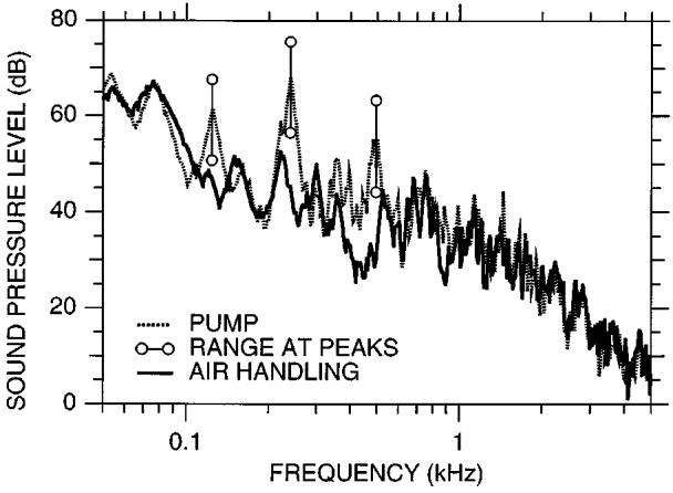
Time-average spectra (unweighted) of noises produced by the combination of the 1.5-T imager coolant pump and the air handling system in the 1.5-T imager room (dotted curve) and the air-handling system alone (solid curve). For the peaks in the pump spectrum at 125, 240, and 490 Hz, the circles connected by vertical bars show the range of levels observed as a 100-ms time window was moved through the 1.7-s pump cycle.
4. Repeatability of gradient noise
For a given set of imaging parameters, the pulse sequence is identical from image acquisition to acquisition, suggesting that the acoustic noise produced by the gradient coils should be highly repeatable. This idea is in agreement with the fact that the spectrum of the highest amplitude gradient noise showed little variability [Figs. 3(C) and (D)]. However, to further examine the degree of noise repeatability, we performed an additional analysis sensitive to waveform timing. For this analysis, the digitized noise waveform from the first acquisition in a 1.5-T measurement session (i.e., the “template waveform”) was subtracted from each of the 16 subsequent noise waveforms recorded during the same session using our standard imaging parameters.26 The amplitudes of the resulting difference waveforms indicated the degree of similarity between each noise waveform and the template waveform, where zero amplitude would indicate that the waveforms were identical in shape and timing. Subtraction of the template waveform reduced the amplitude of the gradient noise waveform at all points in time [Fig. 5(A)]. Lf max at 1 kHz for the difference waveforms was 19-38 dB lower than that for the template noise waveform [Fig. 5(B)].27 L2s was 13-15 dB lower. These reductions indicate that both the gradient noise amplitude and timing were highly repeatable.
FIG. 5.
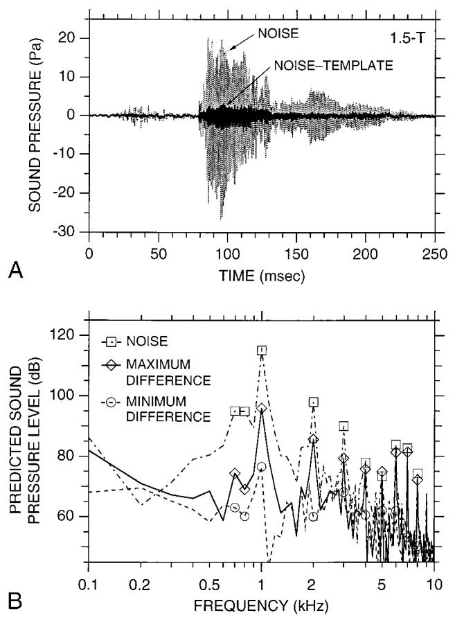
Investigation of the repeatability of gradient coil noise (1.5 T). (A) A noise waveform before (light curve) and after (dark curve) an earlier noise waveform (i.e., a “template waveform”) was subtracted from it. The difference waveform shown (i.e., “noise-template”) had the greatest amplitude of all the difference waveforms calculated in our analyses. (B) Spectra computed over a 10-ms window from the noise waveform in (A) dot-dashed curve, squares), the maximum difference waveform in (A) (solid curve, diamonds), and the minimum difference waveform in our analyses (dashed curve, circles). In each case, the 10-ms window coincided with the waveform peak.
5. Dependence of gradient noise on imaging parameters
Because the readout gradients are the source of the most intense acoustic noise, we expected that Lf max and L2s would be insensitive to changes in the slice-select gradients or to changes in the timing of the readout gradients (i.e., changes that do not alter the amplitude or duration of the readout gradients). This proved to be the case when we examined the effects of varying imaging parameters away from our standard values. For example, when slice orientation was changed (by 90 deg) or slice thickness was changed [from 7 to 3 mm (1.5 T) or from 5 to 3 or 7 mm (3 T], Lf max and L2s were within 1 dB of the values obtained using our standard parameters. These alterations in slice parameters did change the acoustic waveform at the time of the slice-select gradients, which is to be expected since the slice-select gradients control the orientation and thickness of the imaged slice but do not affect the readout gradients. Changes in imaging pulse sequence (from ASE to GE, 1.5 T) are associated with changes in the relative timing of the various gradients and therefore resulted in corresponding changes in the timing of the various components of the acoustic noise waveform. However, for each imager, the readout gradient waveform was the same regardless of pulse sequence. Consequently, Lf max and L2s were insensitive to pulse sequence (i.e., they varied by less than 1 dB).
Doubling the duration of the readout and phase-encode gradient trains,28 from 32 to 64 ms in the 1.5-T imager, did result in an approximately twofold increase in the duration of the highest-amplitude portion of the noise waveform [compare Fig. 6(B) to Fig. 6(A)] and hence an approximate doubling of the energy per 2-s TR. Because the amplitude and frequency of the gradients were unchanged, the level and frequency of Lf max did not change [Fig. 6(C)]. However, the doubling in duration did result in a 2-dB increase in L2s, which is close to the expected value of 3 dB for a doubling in energy.
FIG. 6.
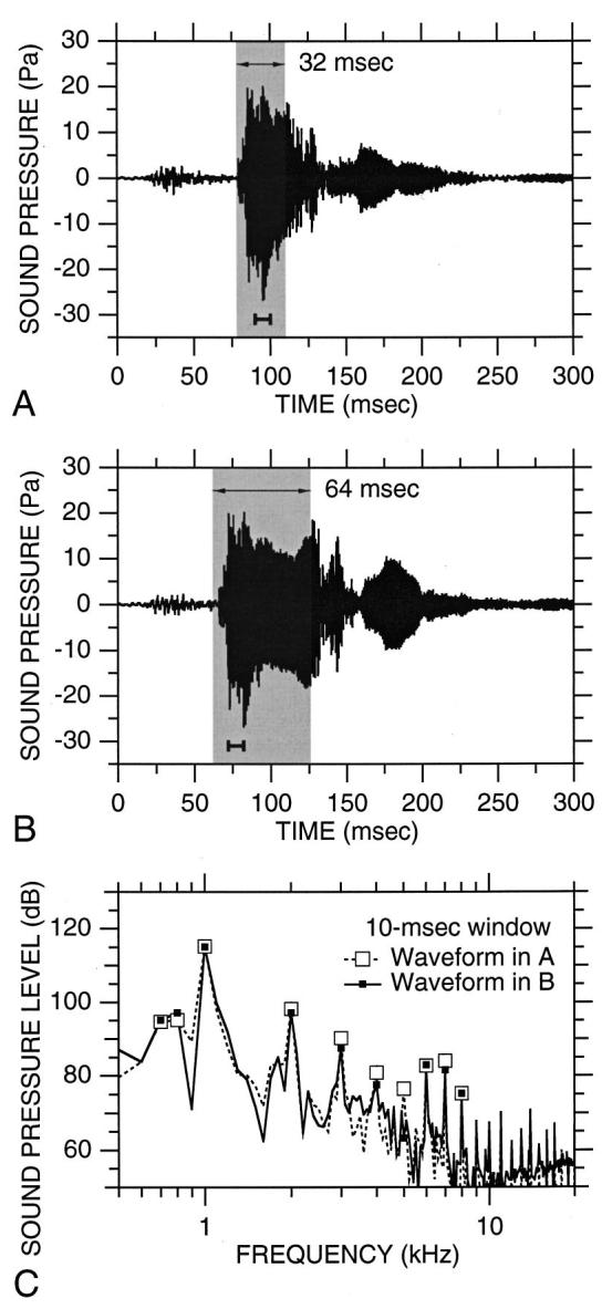
Effect of doubling the duration of the readout and phase-encode gradient trains on the waveform and spectrum of acoustic noise (1.5 T). (A) Noise waveform from Fig. 4(A) obtained using our standard 1.5-T imaging parameters (matrix size 128×64). Gray shading indicates readout and phase-encode gradient activity. (B) Noise waveform obtained using the same parameters as in (A) except that the gradient duration was doubled (matrix size 256×128). (C) Spectrum of waveform in (A) (dashed line, open squares) and waveform in (B) (solid line, filled squares) computed over a 10-ms window coinciding with the peak noise [short bars under waveforms in (A) and (B)].
Increasing the number of slices imaged in a given 2-s time interval did not change Lf max but did increase L2s, because the total gradient noise energy in the time interval increased. Specifically, L2s increased by 7 dB when the number of slices was increased from 1 to 5 and increased by approximately 12 dB when the number of slices was increased from 1 to 15.29 These increases are consistent with five- and 15-fold increases in energy, respectively. In other words, noise energy increased in proportion to the number of slices. This relationship is consistent with our observation that the noise waveforms from successive acquisitions were largely nonoverlapping and thus did not interact with one another to a significant degree, even for the case of 15 slices.30
B. Noise from the pump and air-handling system
The noises produced by the liquid helium pump and the room air-handling system were much lower in both level and frequency than the noise produced by the gradient coils. Figure 7 shows the spectra of noise from the pump and air-handling system for the 1.5-T imager. The pump noise fluctuated cyclically with a period of 1.7 s, showed spectral peaks at 125, 240, and 490 Hz, and decreased in level at higher frequencies. Levels at 240 Hz, the highest spectral peak, fluctuated between 57 and 76 dB SPL (unweighted, when evaluated over a moving 100-ms window, analogous to our analysis technique described in Sec. A 1). The steady-state level of pump and air-handling noise evaluated over the 1.7-s period was 80 dB SPL (unweighted), 71 dB SPL (A-weighted), 79 dB SPL (C-weighted), considerably lower than L2s for the 1.5-T gradient noise with our standard parameters (97 dB SPL). When the pump was turned off, only the air-handling noise remained. The steady-state noise level was then 77 dB SPL (unweighted), 65 dB (A-weighted), 76 dB (C-weighted). The spectrum (computed over 1 s) showed a peak at 80 Hz and decreased with increasing frequency. The pump and air-handling noise spectra and levels in the 3-T imager were similar to the 1.5-T.
IV. DISCUSSION
Our analyses showed that the most intense noise produced by the gradient coils was much higher in level and frequency than the noises produced by the coolant pump and air-handling equipment in the imager room. For the gradient noise, peak levels Lpk of 123 and 138 dB re 20 μPa were observed in a 1.5-T and a 3-T imager, respectively, during EPI-based fMRI. Maximum spectral levels Lfmax were 115 and 131 dB SPL at 1 and 1.4 kHz in the 1.5-T and 3-T imagers; steady-state levels L2s with our standard imaging parameters were 97 and 114 dB SPL (single slice in 2-s period). (These levels, unlike those in previous reports by other authors, were measured without a time weighting.) Noise levels were unchanged by applying either an A- or C-frequency weighting.
The frequency content and timing of the most intense gradient noise indicated that it was primarily attributable to the readout gradients rather than to other gradients in the imaging pulse sequence. This interpretation was supported by the fact that the highest-level noise (a) did not change when imaging parameters were varied in a way that did not affect the readout gradients (e.g., changes in slice thickness or orientation), and (b) changed predictably when the readout gradients were affected (e.g., increasing image matrix size or number of imaged slices).
Noises produced by the coolant pump and air-handling equipment in the imager room were much lower in frequency and level than the gradient noise: 80 dB SPL (unweighted), 71 dB SPL (A-weighted). The fan could be turned off, so there was no point in studying it further.
A. Comparison to previous measurements of fMRI noise
The noise measurements presented in this paper extend previous descriptions of acoustic noise during EPI-based fMRI by providing a more comprehensive description of the spectrum and timing of the noise (previous reports generally included only peak and time-average levels). By computing spectra and levels from digitized waveforms, we have also avoided a limitation of sound-level meters (used in most previous studies) that can cause time-average levels of short-duration sounds to be underestimated.31 We estimate that L2s in the 1.5-T imager, in which the duration of the highest level noise is comparable to the gradient currents (32 ms for our standard parameters), would be underestimated by a sound-level meter by at least 5 dB on the fast setting and at least 13 dB on the slow setting (ANSI S1.4-1985). This potential for underestimation should be kept in mind when comparing our time-average levels with previous reports. Peak levels should be unaffected by differences in measurement method.
Of the four studies reporting noise levels, two included peak levels. Prieto et al. (1998) examined noise levels in a 3-T imager (Bruker Biospec) with a custom insert head gradient system32 for a range of imaging parameters and reported peak levels of 126-139 dB (unweighted), a range that brackets the peak levels measured for the 3-T imager in the present study (137-138 dB). Miyati et al. (1999) reported peak levels of 104-115 dB SPL in nine 1.5-T imagers during single-shot EPI, levels considerably lower than the peak levels in our 1.5-T imager (122-123 dB).
Four previous studies reported time-average noise levels during imaging, measured with a sound-level meter. Prieto et al. (1998) and Miyati et al. (1999) measured time-average A-weighted noise levels (Leq) with a “fast” time weighting. The LA,eq measured by Prieto et al. (1998) in their 3-T imager for a 2-s TR (most analogous to our L2s) was 104 dB SPL. This is approximately 10 dB lower than the A-weighted L2s measured in our 3-T imager (113-114 dB SPL), but roughly 5 dB of the difference may be due to the different measurement methods. Another point of comparison with Prieto et al. (1998) is the effect of increasing the rate at which images were acquired on peak and average noise levels. When Prieto et al. increased the number of images per 2-s interval (by reducing TR from 2 s to as little as 74 ms), peak levels remained constant but average levels increased, similar to our results; however, unlike our results, the increases they observed did not indicate a proportional relationship between noise energy and the number of images acquired. The range of LA,eq measured by Miyati et al. (1999) in their nine imagers (seven slices in a 2.5-s TR) was 92-100 dB SPL, which is lower than our L2s under similar conditions (104 dB for five slices in a 2-s TR).
The two other previous studies reporting noise levels also used a sound-level meter (Cho et al., 1997; Shellock et al., 1998) but did not specify the time weighting used. Levels (C-weighted) reported by Cho et al. (1997) for a General Electric 1.5-T imager (103 dB SPL; TR=3.2 s) are comparable to L2s for our 1.5-T imager. The highest levels (A-weighted) reported by Shellock et al. (1998) for two 1.5-T imagers (General Electric Vision: 115 dB SPL, TR=5 s; Siemens Magnetom: 114 dB; TR=300 ms)33 are considerably higher than L2s in our 1.5-T imager and are very similar to our Lfmax .
Two reports noted the frequency content of the noise during EPI-based fMRI. Cho et al. (1997) presented a noise spectrum from a General Electric 1.5-T imager with a dominant peak at about 1.3 kHz. Miyati et al. (1999) presented octave-band noise spectra (A-weighted) from a General Electric Horizon 1.5-T imager that peaked in the 2-kHz band. In addition, Wessinger et al. (1997) observed that the gradient noise in a Bruker Biospec 3-T imager had a dominant frequency of 2.5 kHz. These studies did not comment on the relationship between these dominant noise frequencies and the gradient activity in their imaging pulse sequence.
B. Noise reduction approaches: Gradient noise
After characterizing the gradient noise during fMRI, we examined ways to reduce the noise. Well-established approaches for reducing unwanted sound offer possibilities in at least four areas: (1) Reduce the noise produced by the gradient coils or by structures that are vibrationally coupled to the gradient coils; (2) Reduce the noise transmitted to the imager bore; (3) Reduce noise at the subject’s ears (using passive hearing protection devices, i.e., earmuffs and/or earplugs); (4) Reduce the noise actively through the introduction of “antinoise” (e.g., Ravicz et al., 1997). In this section we discuss these various noise reduction possibilities in detail.
1. Gradient noise: Reduction at the source
Several approaches have been tried for reducing the gradient noise produced by the imager. Mansfield, Bowtell, and their colleagues (Mansfield et al., 1995; Bowtell and Mansfield, 1995; Bowtell and Peters, 1999) redesigned the coils such that the forces generated by the gradient currents opposed each other (a “force balance”). This reduced gradient noise by 7-15 dB. Cho et al. (1998) replaced the time-varying readout gradients by a constant magnetic field rotated mechanically (the “silent MRI” technique), which reportedly reduced noise levels by 20 dB but imposed constraints on imaging parameters. The effect of these techniques on image quality was not addressed.
Approaches not yet tried can be grouped into two categories. One category involves altering the electrical currents used to set up the gradients, especially the readout gradients since these account for the most intense noise. Perhaps the most direct approach would be to reduce the forces that act on the readout gradient coils by reducing the amplitude of the electrical currents, but doing so would have an adverse effect on image resolution or quality (e.g., Cohen, 1998). If the frequency of the gradient current is sufficiently close to a natural mechanical frequency of the coils34 that their flexure is amplified, the flexure could be reduced by changing the gradient current frequency. However, varying gradient frequency leads to reductions in image quality or resolution due to imaging and equipment constraints (Wald, 1999). If there is indeed a mechanical resonance at 700 Hz (sec. III A 3), then increasing the readout gradient frequency above its current value of 1 kHz might decrease gradient coil flexure and therefore gradient noise.
The second category involves modifying the mechanical properties of the gradient coils, the core on which the coils are wound, or the attachment of the coil/core assembly to the rest of the imager structure. Stiffening the coil/core assembly would reduce flexure unless it also moves natural frequencies of the assembly closer to gradient current frequencies. The natural frequencies of the assembly could be moved further from gradient frequencies by changing the assembly’s stiffness or mass. Mansfield et al. (1998) have proposed relocating the gradient coils on the core and changing the stiffness of the assembly to manipulate its vibration. The assembly’s attachment to the rest of the imager structure could be modified to reduce its motion, though care would have to be taken not to increase the vibration of other parts of the imager because this could degrade image quality (Kelley, 1999) or result in radiated noise into the bore or the room. Active vibration control might reduce coil/core assembly flexure or aid in isolating the rest of the imager structure from vibrations of the assembly. Of the approaches mentioned here, modifications to the mechanical properties of the coil/core assembly or their attachment to the rest of the imager hold the most promise for reducing noise at its source without adversely affecting image quality. Such a solution requires active cooperation of the imager manufacturer.
2. Gradient noise: Reducing transmission
Comparing the frequency content of the most intense gradient noise to the properties of typical sound-attenuating materials indicates that gradient noise transmission from source to subject can be reduced significantly by passive means. In the frequency range of the most intense gradient noise (1-1.4 kHz), sound-attenuating materials such as acoustic barrier-foam composite can provide on the order of 30 dB of attenuation (transmission loss),35 suggesting that the gradient noise reaching a subject could be reduced substantially if attenuating materials were suitably interposed between noise source and subject. A recent experiment confirmed the feasibility of this approach. In this demonstration, a “helmet” made of barrier-foam composite and enclosing the head reduced simulated gradient noise heard by a subject by 15-25 dB (Ravicz and Melcher, 1998a,b).
Preliminary tests suggest that gradient noise transmission can also be reduced by applying passive attenuation materials directly to the imager or imager room (Ravicz et al., 1999). In these tests, noise was measured with a microphone in the bore of the 3-T imager examined in the present study. Lining the bore with barrier-foam composite reduced peak gradient noise levels by approximately 12 dB. This result implies that an important path of noise transmission is directly from source to subject through the walls of the imager bore. That this was not the only important transmission route was shown by an additional test that involved blocking the ends of the bore in addition to lining the bore with acoustic foam (see Fig. 1). Blocking the ends substantially reduced the “resonance and reverberation” part of the noise waveform [after the gradients were turned off, e.g., Fig. 4(A)] recorded within the imager bore, indicating that noise also reaches a subject via a route through the imager room and the ends of the bore. This means that noise transmission to the subject could be reduced further by applying sound-attenuating material to the outer imager shroud to suppress transmission into the imager room, by applying sound-absorbing materials to the walls of the imager room to reduce reverberations, or by applying both treatments. Additional tests indicated that other transmission routes involving vibration of structures inside the bore such as the patient table were less important. Thus, through a combination of passive treatments applied to the most important routes of noise transmission, it is possible to reduce substantially the gradient noise at the location of a subject during fMRI.
3. Gradient noise: Passive hearing protection devices
The simplest and most economical approach for reducing the noise heard by a subject during fMRI is to reduce noise at the ears using passively attenuating earmuffs, earplugs, or both, but there is a limit on the reductions that this approach can provide. Earmuffs and earplugs (when used properly) provide 31-38 and 25-29 dB of attenuation respectively at dominant gradient noise frequencies (1 and 1.4 kHz; Berger, 1983; Berger et al., 1998; Ravicz and Melcher, 1998a, b). However, when the two devices are used together, the reduction in noise heard by a subject (38-43 dB at 1-1.4 kHz) is far less than the sum of the attenuations provided by each device alone. This is because noise conduction through the head and body, though not significant under normal circumstances, becomes a dominant mode of hearing at gradient noise frequencies when earmuffs and earplugs are used together (e.g., Zwislocki, 1957; Berger, 1983; Ravicz and Melcher, 1998a, b). Thus, hearing protection devices alone cannot eliminate the gradient noise heard by a subject during fMRI. Fortunately, this approach can be combined with the other approaches discussed so far.
4. Gradient noise: Active reduction
Several active noise reduction (ANR) systems36 have been developed that reduce gradient noise levels at a subject’s ears (Goldman et al., 1989; Pla et al., 1995; Palmer, 1998). Although these systems demonstrated that a reduction in gradient noise at the ear can be achieved with ANR, this reduction does not necessarily translate into an equal reduction in the noise heard by a subject. This is because ANR applied only at the ear (as with the headset systems of Goldman et al. and Palmer) reduces the noise conducted through the ear canal without reducing conduction through the head and body. For example, in a subject wearing earmuffs and earplugs, ANR at the ear should have virtually no effect on the gradient noise heard because the earmuffs and earplugs reduce noise conduction along the ear canal to the point that conduction through the head and body dominates the noise heard 37 (Ravicz et al., 1998a, b). The free-field system of Pla et al., which reduces noise in a region around the head, may provide additional noise reduction when used with hearing protection devices, but this has not been tested, and noise conduction through the body would still limit the total noise reduction achievable with this system.
The limitation imposed by head and body conduction in applying ANR at the ears could, in theory, be avoided if the gradient noise signal could be canceled at every point on a closed surface encompassing the subject’s head and body. However, implementing a system that approximates this theoretical situation is beyond the scope of today’s technology. The difficulty arises partly because the wavelength of the most intense gradient noise is small compared to the dimensions of the subject, so noise amplitude and phase variations over a surface enclosing the subject would have to be taken into account. Regular bore geometry (Fig. 1), knowledge of gradient coil vibration patterns (e.g., Hedeen and Edelstein, 1997), and the repeatability and predictability of imager noise (sec. III A 4) may eventually make this problem tractable. Given the technical challenges, the other approaches discussed in this section are more practical options for reducing the effects of gradient noise at this time.
C. Noise reduction approaches: Pump- and air-handling noise
Since the pump and air-handling equipment are not essential for imaging, a simple, short-term approach to reducing the noise from these sources is to turn this equipment off temporarily during imaging during particularly noise-sensitive parts of an fMRI experiment. This approach has the drawback that it can be used for only short periods of time. In addition, turning the pump off increases the coolant boiloff rate. It is therefore worth considering alternative approaches.
The four noise reduction possibilities discussed in the previous section are also applicable to the noise produced by the coolant pump and air-handling system. If we assume that minimizing the noise output was not a primary consideration in pump or air-handling system design, substantial reductions in noise at the source may be achievable through simple alterations to this equipment. The use of passive materials to attenuate noise transmission from source to subject or passive hearing protection devices should also be effective approaches. However, they will be less effective in this case than for the case of gradient noise because the pump and air-handling noises are lower in frequency than the gradient noise and passively attenuating materials are less effective at low than high frequencies (Beranek, 1954; Vér and Holmes, 1988). One consequence of this poorer low-frequency performance is that reducing noise at the ear with earmuffs and earplugs does not attenuate low-frequency noise conduction through the ear canal to the point where conduction through the head and body dominates the noise heard (Berger, 1983; Ravicz and Melcher, 1998a, b). This means that ANR applied at the ear can provide a reduction in the (low-frequency) pump and air-handling noise heard by a subject over and above that provided by earmuffs and earplugs, unlike the situation for the higher-frequency gradient noise.38 This, coupled with the fact that ANR is well-suited to reducing low-frequency noise, makes ANR a promising complement to other approaches for reducing the pump and air-handling noise.
D. Importance of noise reduction for all fMRI of brain activity
It is clear that the acoustic background noises present during imaging can adversely affect fMRI studies that use auditory stimuli. However, it may also be that noise affects all fMRI studies of brain activity in as yet unassessed ways. Though the discomfort and anxiety experienced by many patients during conventional MRI is apparently unrelated to the noise (Dantendorfer et al., 1997), the higher noise levels during fMRI could cause discomfort, which may lead to an increase in motion artifacts from unintended head movements that could reduce the detectability of brain activity (Elliott et al., 1999). Noise has been shown to interfere with the performance of some cognitive tasks by reducing a subject’s attentiveness to the task (e.g., Paschler, 1998). Since changes in attentiveness have been demonstrated to affect brain activity (Woodruff et al., 1996), the noise potentially can affect the results of any fMRI study of subject performance or response to any stimulus, not just auditory stimuli. Two studies have reported different effects of increasing time-average noise levels during nonauditory tasks (Elliott et al., 1999; Cho et al., 1998), but no study to date has examined the effect of reducing the noise. This issue will mostly likely remain unresolved until quieter imaging facilities are available.
V. CONCLUSIONS
The nature of the high noise levels present during fMRI makes total elimination of imager noise perceived by subjects impractical at this time. However, significant noise reduction is possible using existing methods.
Because noise levels are high and the gradient noise and the pump- and air-handling noise occupy different parts of the frequency spectrum, substantial noise reduction will undoubtedly require a combination of approaches.
Substantial reductions in gradient noise levels have been demonstrated using passive noise reduction approaches such as hearing protection devices (earmuffs and earplugs) or the use of noise attenuation material to reduce noise transmission from the gradient coils to the subject. This result is to be expected, since these approaches are more effective for high-frequency components than low.
Although MRI-compatible active noise reduction (ANR) systems have been developed, they are less effective at reducing high-frequency gradient noise than passive techniques and therefore seem less practical for most applications. The effectiveness of present ANR systems in conjunction with hearing protection devices that reduce sound conduction through the ear canal (e.g., an ANR headset) is limited by noise conducted through the head and body that bypasses these treatments. To solve this problem, ANR must be applied over the subject’s head and body, an approach that cannot be implemented with present technology.
Pump noise levels can also be reduced by passive noise reduction approaches and could probably be eliminated by appropriate pump design and placement. Because the effectiveness of ANR increases at low frequencies, ANR may be a more effective option for reducing pump- and air-handling noise than passive techniques.
Even a combination of approaches is unlikely to reduce unwanted sounds to levels below the threshold of hearing. Therefore, optimal imaging conditions can be achieved only by redesigning the imaging equipment to reduce the noise at its sources.
ACKNOWLEDGMENTS
The authors wish to thank Douglas Kelley at ANMR, General Electric Medical Systems, and MGH for many helpful discussions on the sources of imager noise; Larry L. Wald, Terence A. Campbell, Whitney B. Edmister, Thomas M. Talavage, Bruce Rosen, and Randy Benson at the MGH Imaging Center for technical information and support; John J. Guinan, William T. Peake, John J. Rosowski, Mark N. Oster, and Larry L. Wald for comments on earlier versions of the manuscript; Knowles Electronics for supplying microphones; Barbara E. Norris for assistance in document preparation; and the staff of the Eaton-Peabody Laboratory for general help. Supported by NIH/NIDCD No. P01 DC00119.
Footnotes
Time-average noise levels (root-mean-square sound pressure over a given time interval, expressed in dB re 20 μPa—ANSI S1.1-1994) used for assessing noise hazard include a time weighting (e.g., fast, slow) that deemphasizes sudden changes in level and a frequency weighting (e.g., A,C) that relates sound levels to human loudness curves (e.g., Earshen, 1986). A-weighted sound levels have been shown to be a good predictor of observed threshold shifts and hearing losses (e.g., von Gierke and Nixon, 1992).
Note that these imagers did not include the noise-attenuating material under the imager shroud which is sometimes supplied with GE Signa imagers. When installed, this material reportedly reduces noise by 5 dB (Counter et al., 1997).
Our measurement technique differs slightly from the National Electrical Manufacturers Association (NEMA) MS 4 maximum clinical acoustic noise (MCAN) procedure in that (1) our microphones were positioned approximately at the location of a subject’s ears rather than at the imager isocenter; (2) we digitized waveforms instead of using a sound meter, which allowed us to compute accurate noise spectra; (3) we measured noise in a typical imaging paradigm rather than with maximal gradient activity; and (4) our imager bore contained a phantom. In fact, the primary frequencies of imager noise are sufficiently high that the sound pressure probably varies over the volume of the bore [for instance, Hedeen and Edelstein (1997) and Shellock et al. (1998) measured differences in sound pressure of several dB between the center and the ends of the bore, all on the bore axis, and we have observed differences in sound pressure between the axis of the (empty) bore and a point approximately 10 cm off-axis]. To our knowledge, no systematic study of the sound field over the entire bore has been performed. Noise levels measured approximately at the location of the ears with a phantom in place (which serves as a dummy head for this purpose), rather than at the center of the symmetric bore, may provide a more realistic estimate of the actual noise levels experienced by subjects in the imager.
The slice would have been approximately parallel to the Sylvian fissure in a supine subject.
TE=70 ms, offset=-25 ms, field of view (FOV)=40×20 cm, frequency-encode direction: right-left.
TE=35 ms, FOV=40×20 cm, frequency-encode direction: right-left.
The slice would have been approximately perpendicular to the Sylvian fissure in a supine subject.
TE=50 ms, flip angle=90 deg, FOV=40×20 cm, frequency-encode direction: right-left.
Care was taken not to let the tape touch the microphone diaphragm.
Both the Shure and the Knowles microphone had integral preamps that provided a low-impedance output.
Harmonic distortion at 1.4 kHz (the primary frequency of the gradient noise at 3 T) would presumably be comparable to that at 1 kHz because harmonic distortion for condenser microphones is typically fairly constant across frequency (e.g., Zuckerwar, 1995).
Microphone outputs in response to a 250-Hz pistonphone source were reduced by at least 40 dB when the microphones were encased in clay. (Note that the clay did not touch the microphone diaphragm and that the microphones were immersed in the sound field within the pistonphone cavity for these measurements.) We know that the clay did not damage the microphones because microphone outputs were the same after removing the clay as before applying the clay.
Encasing the microphone in this way may be a more rigorous test of artifact than using a dummy microphone, in that the measurement microphone is still in place and functional. Several other investigators have also established that condenser microphones are largely immune to electrical artifact in the imager (e.g., Hurwitz et al., 1989; Shellock et al., 1994; Counter et al., 1997).
For computations of time-average levels, the waveform was high-pass filtered at 240 Hz to minimize the artifact.
The sound-pressure waveforms p[t] (sound pressure as a function of time t) shown were computed from the microphone voltage output waveform w[t] by dividing w[t] by the microphone sensitivity rm (in V/Pa) measured in a pistonphone at 250 Hz.
For the sound-pressure waveform p[t], the peak level , where ppk is the maximum of |p[t]| (ANSI S1.13-1995).
For this waveform with time-varying amplitude, a 10-ms window provided a good combination of time and frequency resolution. The 10-ms waveform segment included an integral number of cycles at the frequency of the peak in the noise spectrum, which allowed us to use a rectangular window to minimize spectral smearing (e.g., Oppenheim and Schafer, 1989).
For the ith 10-ms (N-point) windowed waveform segment wi[t], the sound-pressure spectrum Spi[f] (in Pa) was computed from the Fourier transform Si[f] of wi[t] and the frequency response of the microphone and amplifier Sm[f] (V/Pa) by . Shown in Figs. 3(C) and (D) is the spectrum containing Lf max for positive frequencies, divided by to obtain root-mean-square pressures and expressed in dB SPL.
Note that Lf max is defined slightly differently from the “maximum sound level” or “spectral level” described in ANSI S1.1 (1994). We call Lf max the “maximum spectral level” because this term has the same sense as the ANSI terms: the highest of spectral levels computed over short time intervals.
Time-average noise levels were derived from the acoustic energy in the noise signal (—see ANSI S1.1-1994). For our calculations T was either 10 ms or 2 s. We chose to compute time-average levels from the energy in the sound pressure spectrum SpT[f] rather than the time waveform p[t] because correcting for the nonflat frequency response of our microphones was easier in the frequency domain; the two methods are equivalent by Parseval’s theorem (Oppenheim and Schafer, 1989). For example, the time-average level over a 2-s time window L2s (N points) was computed from the sound-pressure spectrum over the 2-s interval Sp2s by .
With one exception: For the last measurement in session II in the 3 T, Lf max underestimated the time-average noise level over the 10-ms window containing Lf max by less than 2 dB.
Normally, the chemical-saturation gradient would be preceded by an rf pulse, and each of the slice-select gradients would be centered on an rf pulse. For these measurements, the rf transmitter was disconnected.
The readout and phase-encode gradients were each immediately preceded by a 1-ms pulse, and the phase-encode gradient was followed by a 5-ms pulse (not shown in Fig. 4).
Time for 60-dB decay T60≈0.161 V/a, where V is the volume of the room, the mean absorption , and Si and αi are the area and absorption coefficient, respectively, of each plaster wall, the acoustical tile ceiling, and the concrete floor. Absorption coefficients from Kinsler et al., 1982.
An experiment in the 3-T imager suggested that most of the noise in the bore 20 ms or more after the switch-off of the gradient currents was due to room reverberation (Ravicz et al., 1999).
For these calculations, the trigger pulses (from the imager controller, to which the noise and template waveforms were synchronized) were aligned, and the waveforms were subtracted on a sample-by-sample basis.
This may be a conservative estimate of the reduction achievable because of uncertainty in our measurements of the timing of the imager trigger: Measurements of trigger timing had an uncertainty of 21 μs due to the 48-kHz sample rate of our A/D converter.
This was accomplished by changing the image matrix size from 128×64 to 256×128.
Note that when multiple (5 or 15) slices were specified, there was a corresponding number of equally spaced image acquisitions (one per slice) during each TR.
The noise waveforms for successive image acquisitions were largely nonoverlapping because the time between acquisitions [repetition time (TR)/number of slices=2 s/15=133 ms] was comparable to the duration (∼140 ms) of the highest-amplitude noise in the 1.5-T imager [occurring between roughly 80 and 220 ms in Fig. 4(A)].
Though sound-level meters provide a quick and simple way of estimating average noise levels, the most commonly used meter time weighting settings (fast and slow) are inherently not well-suited for accurate time-average measurements of short-duration sound (e.g., ANSI S1.13-1995). The fact that the time constants associated with these settings (fast: 125 ms; slow: 1 s) are comparable to or longer than the duration of our high-level imager noise means that time-average noise levels, if measured with these settings, could have been significantly underestimated (ANSI S1.4-1985; Earshen, 1986).
The insert gradient coil was designed and fabricated at the Medical College of Wisconsin Biophysics Research Institute and is approximately 33 cm in diameter, considerably smaller than the scanner bore (Prieto, 1999).
Note that the field of view was also varied among these measurements. Prieto et al. (1998) have shown that FOV influences noise levels.
For example, the apparent resonance at 700 Hz observed in our 1.5-T imager—see Sec. III C.
For example, E·A·R E-0-10-25 (see E·A·R, 1999).
Active noise reduction (ANR) involves introducing an acoustic signal (“antinoise”) into a noise field that combines destructively with the noise. Of the two main ANR strategies (feedforward and feedback), most commercial ANR headsets use a feedback strategy (e.g., Olson and May, 1953) in which noise is sensed at a particular location and antinoise is computed and delivered to the sensing location in “real time.” There is, however, an inherent delay due to processing time that causes the noise and antinoise to become out of phase as frequency increases; hence, with increasing frequency, the antinoise produces a diminishing reduction and eventually an amplification of the noise (e.g., Elliott and Nelson, 1993). Since the effectiveness of such ANR systems decreases as frequency increases, systems using this strategy are inherently less suitable for reducing the most intense gradient noise (e.g., 1 kHz and above). [For instance, the effectiveness of most commercial ANR headsets decreases above a few hundred hertz, and most are ineffective above 1 kHz (e.g., Casali and Berger, 1996).] Alternatively, if the timing of the noise is predictable (such as for the gradient noise), the time delay problem can be overcome by synchronizing the antinoise to the imager controller—a feedforward approach (e.g., Lueg, 1936; Elliott and Nelson, 1993; Fuller and von Flotow, 1995). The antinoise itself can be synthesized from measured transfer functions between the gradient current and the resulting sound (e.g., Hedeen and Edelstein, 1997) or can be an inverted copy of a previously measured noise waveform. All ANR systems developed for MRI to date have employed a feedforward strategy.
In support of this idea, Palmer and his colleagues have observed that, for subjects wearing their ANR headset, reductions in the noise heard were smaller than the reduction in noise level at the entrance of the ear canal at frequencies above 1 kHz (Palmer, 1998).
In the frequency range of pump and air-handling noise (<500 Hz), commercially available ANR headsets (using feedback control) typically provide 10-20 dB additional noise reduction at the ear (e.g., Casali and Berger, 1996). Though not currently magnet-compatible, these headsets could be adapted for use during MRI. ANR with feedforward control may also be appropriate because the pump noise is periodic.
Portions of this material were presented at the 1997 American Speech-Language-Hearing Association meeting, Boston, MA, 23 November 1997, the Twentieth and Twenty-first Midwinter Meetings of the Association for Research in Otolaryngology, St. Petersburg Beach, FL, 5 February 1997 and 18 February 1998, and the Fourth International Conference on Functional Mapping of the Human Brain, Montreal, PQ Canada, 11 June 1998.
References
- ANSI . Specification for Sound Level Meters (amended) American National Standards Institute; New York: 1985. S1.4. [Google Scholar]
- ANSI . Acoustical Terminology. American National Standards Institute; New York: 1994. S1.1. [Google Scholar]
- ANSI . Measurement of Sound Pressure Levels in Air. American National Standards Institute; New York: 1995. S1.13. [Google Scholar]
- Bandettini PA, Jesmanowicz A, Van Kylen J, Birn RM, Hyde JS. Functional MRI of brain activation induced by scanner acoustic noise. Magn. Reson. Med. 1998;39:410–416. doi: 10.1002/mrm.1910390311. [DOI] [PubMed] [Google Scholar]
- Beranek LL. Acoustics. McGraw-Hill; New York: 1954. p. 481. [Google Scholar]
- Berger EH. Laboratory attenuation of earmuffs and earplugs both singly and in combination. Am. Ind. Hyg. Assoc. J. 1983;44:321–329. [Google Scholar]
- Berger EH, Franks JR, Behar A, Casali JG, Dixon-Ernst C, Kieper RW, Merry CJ, Mozo BT, Nixon CW, Ohlin D, Royster JD, Royster LH. Development of a new standard laboratory protocol for estimating the field attenuation of hearing protection devices. III. The validity of using subject-fit data. J. Acoust. Soc. Am. 1998;103:665–672. doi: 10.1121/1.423236. [DOI] [PubMed] [Google Scholar]
- Bowtell RW, Mansfield P. Quiet transverse gradient coils: Lorentz force balanced designs using geometrical similitude. Magn. Reson. Med. 1995;34:494–497. doi: 10.1002/mrm.1910340331. [DOI] [PubMed] [Google Scholar]
- Bowtell RW, Peters A. Analytic approach to the design of transverse gradient coils with co-axial return paths. Magn. Reson. Med. 1999;41:600–608. doi: 10.1002/(sici)1522-2594(199903)41:3<600::aid-mrm24>3.0.co;2-e. [DOI] [PubMed] [Google Scholar]
- Brummett RE, Talbot JM, Charuhas P. Potential hearing loss resulting from MR imaging. Radiology. 1988;169:539–540. doi: 10.1148/radiology.169.2.3175004. [DOI] [PubMed] [Google Scholar]
- Bushong SC. Magnetic Resonance Imaging: Physical and Biological Principles. 2nd ed. Mosby, St; Louis: 1996. p. 497. [Google Scholar]
- Casali JG, Berger EH. Technology advancements in hearing protection circa 1995: Active noise reduction, frequency/amplitude sensitivity, and uniform attenuation. Am. Ind. Hyg. Assoc. J. 1996;57:175–185. doi: 10.1080/15428119691015115. [DOI] [PubMed] [Google Scholar]
- Cho ZH, Chung ST, Chung JY, Park SH, Kim JS, Moon CH, Hong IK. A new silent magnetic resonance imaging using a rotating dc gradient. Magn. Reson. Med. 1998;39:317–321. doi: 10.1002/mrm.1910390221. [DOI] [PubMed] [Google Scholar]
- Cho ZH, Park SH, Kim JH, Chung SC, Chung ST, Chung JY, Moon CW, Yi JH, Sin CH, Wong EK. Analysis of acoustic noise in MRI. Magn. Reson. Imaging. 1997;15:815–822. doi: 10.1016/s0730-725x(97)00090-8. [DOI] [PubMed] [Google Scholar]
- Cohen M. Theory of echo-planar imaging. In: Schmitt F, Stehling MK, Turner R, editors. Echo-Planar Imaging: Theory, Technique and Application. Springer; Berlin: 1998. pp. 11–30. [Google Scholar]
- Counter SA, Olofsson Å, Grahn HF, Borg E. MRI acoustic noise: Sound pressure and frequency analysis. JMRI. 1997;7:606–611. doi: 10.1002/jmri.1880070327. [DOI] [PubMed] [Google Scholar]
- Dantendorfer K, Amering M, Bankier A, Helbich T, Prayer D, Youssefzadeh S, Alexandrowicz R, Imhof H, Katschnig H. A study of the effects of patient anxiety, perceptions and equipment on motion artifacts in magnetic resonance imaging. Magn. Reson. Imaging. 1997;15:301–306. doi: 10.1016/s0730-725x(96)00385-2. [DOI] [PubMed] [Google Scholar]
- E·A·R. Materials Summary Sheet MSS3 Barrier Composites. E·A·R Specialty Composites, Indianapolis IN. 1999Available at 〈http://www.earsc.com/new/pdfs/mss/BarrCompositesMSS3.pdf〉. Viewed 30 August 2000.
- Earshen JJ. Sound measurement: Instrumentation and noise descriptors. In: Berger EH, Ward WD, Morrill JC, Royster LH, editors. Noise and Hearing Conservation Manual. American Industrial Hygiene Association; Akron, OH: 1986. pp. 37–95. [Google Scholar]
- Eden GF, Joseph JE, Brown HE, Brown CP, Zeffiro TA. Utilizing hemodynamic delay and dispersion to detect fMRI signal change without auditory interference: The behavior interleaved gradients technique. Magn. Reson. Med. 1999;41:13–20. doi: 10.1002/(sici)1522-2594(199901)41:1<13::aid-mrm4>3.0.co;2-t. [DOI] [PubMed] [Google Scholar]
- Edmister WB, Talavage TM, Ledden PJ, Weisskoff RM. Improved auditory cortex imaging using clustered volume acquisitions. Hum. Brain Mapp. 1999;7:89–97. doi: 10.1002/(SICI)1097-0193(1999)7:2<89::AID-HBM2>3.0.CO;2-N. [DOI] [PMC free article] [PubMed] [Google Scholar]
- Elliott MR, Bowtell RW, Morris PG. The effect of scanner sound in visual, motor, and auditory functional MRI. Magn. Reson. Med. 1999;41:1230–1235. doi: 10.1002/(sici)1522-2594(199906)41:6<1230::aid-mrm20>3.0.co;2-1. [DOI] [PubMed] [Google Scholar]
- Elliott SJ, Nelson PA. Active noise control. IEEE Signal Process. Mag. 1993;10(4):12–35. [Google Scholar]
- Fuller CR, von Flotow AH. Active control of sound and vibration. IEEE Control Syst. Mag. 1995;15(6):9–19. [Google Scholar]
- Goldman AM, Gossman WE, Friedlander PC. Reduction of sound levels with antinoise in MR imaging. Radiology. 1989;171:549–550. doi: 10.1148/radiology.173.2.2798889. [DOI] [PubMed] [Google Scholar]
- Hall DA, Haggard MP, Akeroyd MA, Palmer AR, Summerfield AQ, Elliott MR, Gurney E, Bowtell RW. Sparse’ temporal sampling in auditory fMRI. Hum. Brain Mapp. 1999;7:213–223. doi: 10.1002/(SICI)1097-0193(1999)7:3<213::AID-HBM5>3.0.CO;2-N. [DOI] [PMC free article] [PubMed] [Google Scholar]
- Hedeen RA, Edelstein WA. Characterization and prediction of gradient acoustic noise in MR imagers. Magn. Reson. Med. 1997;37:7–10. doi: 10.1002/mrm.1910370103. [DOI] [PubMed] [Google Scholar]
- Hurwitz R, Lane SR, Bell RA, Brant-Zawadzki MN. Acoustic analysis of gradient-coil noise in MR imaging. Radiology. 1989;173:545–548. doi: 10.1148/radiology.173.2.2798888. [DOI] [PubMed] [Google Scholar]
- Kelley, Douglas AC. 1994. Personal communication to M.E.R. and J.R.M.
- Kelley, Douglas AC. 1999. Personal communication to M.E.R.
- Kinsler LE, Frey AR, Coppens AB, Saunders JV. Fundamentals of Acoustics. 3rd ed. Wiley; New York: 1982. p. 480. [Google Scholar]
- LABVIEW, Version 2. National Instruments; Austin, TX: 1991. [Google Scholar]
- Lueg P. 1936. “Process of silencing sound oscillations,” U.S. Patent 2,043,416, 19 June 1936.
- Mansfield P, Chapman BLW, Bowtell R, Glover P, Coxon R, Harvey PR. Active acoustic screening: Reduction of noise in gradient coils by Lorentz force balancing. Magn. Reson. Med. 1995;33:276–281. doi: 10.1002/mrm.1910330220. [DOI] [PubMed] [Google Scholar]
- Mansfield P, Glover PM, Beaumont J. Sound generation in gradient coil structures for MRI. Magn. Reson. Med. 1998;39:539–550. doi: 10.1002/mrm.1910390406. [DOI] [PubMed] [Google Scholar]
- MATLAB, Version 5.2 for Macintosh. The Mathworks; Natick, MA: 1998. [Google Scholar]
- McJury MJ. Acoustic noise levels generated during high field MR imaging. Clin. Radiol. 1995;50:331–334. doi: 10.1016/s0009-9260(05)83427-0. [DOI] [PubMed] [Google Scholar]
- McJury MJ, Blug A, Joerger C, Condon B, Wyper D. Acoustic noise levels during magnetic resonance imaging scanning at 1.5 T. Br. J. Radiol. 1994;67:413–415. doi: 10.1259/0007-1285-67-796-413. [DOI] [PubMed] [Google Scholar]
- Melcher JR, Talavage TM, Harms MP. Functional MRI of the Auditory System. In: Moonen C, Bandettini P, editors. Medical Radiology, Diagnostic Imaging and Radiation Oncology: Functional MRI. springer; Berlin: 1999. pp. 393–406. [Google Scholar]
- Miyati T, Banno T, Fujita H, Mase M, Narita H, Imazawa M, Ohba S. Acoustic noise analysis in echo planar imaging: Multicenter trial and comparison with other pulse sequences. IEEE Trans. Med. Imaging. 1999;18:733–736. doi: 10.1109/42.796286. [DOI] [PubMed] [Google Scholar]
- NEMA . Acoustic Noise Measurement Procedure for Diagnostic Magnetic Resonance Imaging Devices. National Electrical Manufacturers Association; Washington, DC: 1989. MS 4-1989: [Google Scholar]
- OSHA . OSHA Regulations (Standards-29 CFR), Occupational noise exposure-1910.95. Occupational Safety and Health Administration; Washington, DC: 1996. , 7 March 1996. Available: 〈http://www.osha-slc.gov/OshStd_data/1910_0095.html〉. Viewed 4 May 2000.
- Olson HF, May EG. Electronic sound absorber. J. Acoust. Soc. Am. 1953;25:1130–1136. [Google Scholar]
- Oppenheim AV, Schafer RW. Discrete-Time Signal Processing. Prentice-Hall; Englewood Cliffs, NJ: 1989. p. 879. [Google Scholar]
- Palmer AR, Bullock DC, Chambers JD. A high-output, high-quality sound system for use in auditory fMRI. NeuroImage. 1998;7(4):S359. [Google Scholar]
- Palmer AR. 1998. Personal communication to M.E.R.
- Paschler HE. The Psychology of Attention. MIT Press; Cambridge, MA: 1998. p. 494. [Google Scholar]
- Pla FG, Sommerfeldt SD, Hedeen RA. Proceedings of Active 95. Noise Control Foundation; Poughkeepsie, NY: 1995. Active control of noise in magnetic resonance imaging; pp. 573–582. [Google Scholar]
- Prieto TE, Bennett K, Weyers D. Acoustic noise levels in a head gradient coil during echo planar imaging; Proceedings of the International Society for Magnetic Resonance in Medicine, Sixth Scientific Meeting and Exhibition; 1998.p. 750. [Google Scholar]
- Prieto TE. 1999. Personal communication to M.E.R.
- Ravicz ME, Melcher JR. Abstracts of the Twenty-first Midwinter Meeting of the Association for Research in Otolaryngology. ARO, Mt.; Royal, NJ: 1998a. Reducing imager-generated noise at the ear during functional magnetic resonance imaging: Passive attenuation; p. 208. [Google Scholar]
- Ravicz ME, Melcher JR. Imager noise and noise reduction during fMRI. NeuroImage. 1998b;7(4):S556. [Google Scholar]
- Ravicz ME, Melcher JR, Talavage TM, Benson RR, Rosen BR, Kiang NYS. Abstracts of the Twentieth Midwinter Meeting of the Association for Research in Otolaryngology. ARO, Des Moines; IA: 1997. Characterization and reduction of imager-generated noise during functional magnetic resonance imaging (fMRI) p. 205. [Google Scholar]
- Ravicz ME, Melcher JR, Wald LL. Reducing acoustic noise transmission from gradient coils to subject during fMRI: An approach and preliminary results. Neuroimage. 1999;9:S1. [Google Scholar]
- Savoy RL, Ravicz ME, Gollub R. The Psychophysiological Laboratory in the Magnet: Stimulus Delivery, Response Recording, and Safety. In: Moonen C, Bandettini P, editors. Medical Radiology, Diagnostic Imaging and Radiation Oncology: Functional MRI. springer; Berlin: 1999. pp. 347–365. [Google Scholar]
- Schmitt F, Irnich W, Fischer H. Physiological side effects of fast gradient switching. In: Schmitt F, Stehling MK, Turner R, editors. Echo-Planar Imaging: Theory, Technique and Application. springer; Berlin: 1998. pp. 201–252. [Google Scholar]
- Shah NJ, Jäncke L, Grosse-Ruyken M-L, Müller-Gärtner HW. Influence of acoustic masking noise in fMRI of the auditory cortex during phonetic discrimination. JMRI. 1999;9:19–25. doi: 10.1002/(sici)1522-2586(199901)9:1<19::aid-jmri3>3.0.co;2-k. [DOI] [PubMed] [Google Scholar]
- Shellock FG, Morisoli SM, Ziarati M. Measurement of acoustic noise during MR imaging: Evaluation of six ‘worst-case’ pulse sequences. Radiology. 1994;191:91–93. doi: 10.1148/radiology.191.1.8134603. [DOI] [PubMed] [Google Scholar]
- Shellock FG, Ziarati M, Atkinson D, Chen D-Y. Determination of acoustic noise during MRI using echo planar and three dimensional, fast spin echo techniques. JRMI. 1998;8:1154–1157. doi: 10.1002/jmri.1880080522. [DOI] [PubMed] [Google Scholar]
- Talavage TM, Edmister WB, Ledden PJ, Weisskoff RM. Quantitative assessment of auditory cortex responses induced by imager acoustic noise. Hum. Brain Mapp. 1999;7:79–88. doi: 10.1002/(SICI)1097-0193(1999)7:2<79::AID-HBM1>3.0.CO;2-R. [DOI] [PMC free article] [PubMed] [Google Scholar]
- Ulmer JL, Biswal BB, Yetken FZ, Mark LP, Mathews VP, Prost RW, Estkowski LD, McAuliffe TL, Haughton VM, Daniels DL. Cortical activation response to acoustic echo planar scanner noise. J. Comput. Assist. Tomogr. 1998;22:111–119. doi: 10.1097/00004728-199801000-00021. [DOI] [PubMed] [Google Scholar]
- Vér IL, Holmes CI. Interaction of sound waves with solid structures. In: Beranek LL, editor. Noise and Vibration Control. Institute of Noise Control Engineering; Washington, DC: 1988. pp. 270–361. [Google Scholar]
- Von Gierke, Nixon CW. Damage risk criteria for hearing and human body vibration. In: Beranek LL, Vér IL, editors. Noise and Vibration Control Engineering: Principles and Applications. wiley; New York: 1992. pp. 585–616. [Google Scholar]
- Wald LL. 1999. Personal communication to M.E.R. and J.R.M.
- Wessinger CM, Buonocore MH, Kussmaul CL, Mangun GR. Tonotopy in human auditory cortex examined with functional magnetic resonance imaging. Hum. Brain Mapp. 1997;5:18–25. doi: 10.1002/(SICI)1097-0193(1997)5:1<18::AID-HBM3>3.0.CO;2-Q. [DOI] [PubMed] [Google Scholar]
- Woodruff PWR, Benson RR, Bandettini PA, Kwong KK, Howard RJ, Talavage T, Belliveau J, Rosen BR. Modulation of auditory and visual cortex by selective attention is modality-dependent. NeuroReport. 1996;7:1909–1913. doi: 10.1097/00001756-199608120-00007. [DOI] [PubMed] [Google Scholar]
- Zuckerwar AJ. Principles of operation of condenser microphones. In: Wong GSK, Embleton TFW, editors. AIP Handbook of Condenser Microphones. AIP; Woodbury, NY: 1995. pp. 37–69. [Google Scholar]
- Zwislocki J. In search of the bone-conduction threshold in a free sound field. J. Acoust. Soc. Am. 1957;29:795–804. [Google Scholar]