

Abstract
Objective
Arsenic is a pervasive contaminant in underground aquifers worldwide, yet documentation of health effects associated with low-to-moderate concentrations (<100 μg/L) has been stymied by uncertainties in assessing long-term exposure. A critical component of assessing exposure to arsenic in drinking water is the development of models for predicting arsenic concentrations in private well water in the past; however, these models are seldom validated. The objective of this paper is to validate alternative spatial models of arsenic concentrations in private well water in southeastern Michigan.
Methods
From 1993−2002 the Michigan Department of Environmental Quality analyzed arsenic concentrations in water from 6,050 private wells. This dataset was used to develop several spatial models of arsenic concentrations in well water: proxy wells based on nearest neighbor relationships, averages across geographic regions, and geostatistically-derived estimates based on spatial correlation and geologic factors. Output from these models was validated using arsenic concentrations measured in 371 private wells from 2003−2006.
Results
The geostatisical model and nearest neighbor approach outperformed the models based on geographic averages. The geostatistical model produced the highest degree of correlation using continuous data (Pearson's r=0.61; Spearman's rank ρ=0.46) while the nearest neighbor approach produced the strongest correlation (κweighted=0.58) using an a priori categorization of arsenic concentrations (<5, 5−9.99, 10−19.99, ≥20 μg/L). When the maximum contaminant level was used as a cut-off in a two-category classification (<10, ≥10 μg/L), the nearest neighbor approach and geostatistical model had similar values for sensitivity (0.62−0.63), specificity (0.80), negative predictive value (0.85), positive predictive value (0.53), and percent agreement (75%).
Discussion
This validation study reveals that geostatistical modeling and nearest neighbor approaches are effective spatial models for predicting arsenic concentrations in private well water. Further validation analyses in other regions are necessary to indicate how widely these findings may be generalized.
Keywords: Arsenic, Drinking water, Exposure assessment, Environmental epidemiology, Spatial analysis
INTRODUCTION
Elevated levels of arsenic in drinking water have been detected in nearly every country, with concentrations frequently exceeding the World Health Organization guideline and United States (US) maximum contaminant level (MCL) of 10 μg/L in many places, including the Bengal basin, the Mekong basin, Taiwan, Chile, and Argentina (Smedley and Kinniburgh, 2002). Arsenic occurs naturally in groundwater from dissolution of arsenic-bearing mineral constituents in underground aquifers, with concentrations typically ranging from <1−1000 μg/L. Elevated levels of arsenic are cause for concern because arsenic is associated with a number of adverse health outcomes, including several types of cancer, vascular diseases, dermatological ailments, diabetes, respiratory diseases, cognitive decline, and infant mortality (Chen et al., 1995; Chiou et al., 1997; Hopenhayn-Rich et al., 2000; Mazumder et al., 2005; Rahman et al., 1998; Rahman et al., 2006; Tseng, 1977; Wasserman et al., 2004; Yang et al., 2003).
Mobilization of arsenic from geological formations into groundwater is driven by a host of biogeochemical and hydrologic factors. These factors include sediment mineralogy, well depth, microbial oxidation or reduction of arsenic, competing elemental species for sorption sites, groundwater recharge, groundwater flow path, and presence of fractures in bedrock formations (Ayotte et al., 2006; Ford et al., 2006; Harvey et al., 2006; Smedley and Kinniburgh, 2002; Van Geen et al., 2003; van Geen et al., 2006). These factors are often highly variable between wells and therefore have been difficult to incorporate into models for predicting arsenic concentrations in well water (Ayotte et al., 2006; Van Geen et al., 2006).
In epidemiological studies, accurate and reliable estimates of arsenic concentrations at previously used wells are critical for assessing exposure in individuals who change residences and water sources. Given the challenges in building predictive models based on biogeochemical and hydrologic factors, research teams have adopted a variety of spatial modeling techniques for predicting arsenic concentrations in private wells. These models rely on the spatial pattern of measured arsenic concentrations in generating predictions. For example, studies of lung cancer, bladder cancer, and hypertension in Taiwan relied on average levels of arsenic in well water in villages to estimate past exposure (Chen et al., 1995; Chen et al., 2003; Chen et al., 2004). In a bladder cancer study conducted in the western US, arsenic concentrations were averaged for all wells within the same geographic region (US Public Land Survey-defined Sections) and of similar depth as a well from a past residence (Steinmaus et al., 2003). In an Argentinean study of bladder cancer, proxy wells drilled into a common aquifer were used to estimate arsenic concentrations for a past residence (Bates et al., 2004). In Michigan and Bangladesh, geostatistical models were developed to predict arsenic concentrations in well water (Goovaerts et al., 2005; Hassan et al., 2003; Serre et al., 2003). The predictive capacity of these different spatial models, however, has yet to be evaluated.
Arsenic concentrations in groundwater as high as 335 μg/L were first reported in southeastern Michigan in 1981 (MDPH, 1982). Since then, arsenic has been identified in unconsolidated and bedrock aquifers throughout southeastern Michigan, with concentrations frequently exceeding the US MCL (Haack and Treccani, 2000; Kim et al., 2002; Slotnick et al., 2006). This region has a population of about 2.8 million people, with 1.6 million people relying on groundwater as their drinking water source, and an estimated 230,000 people exposed to arsenic ≥10 μg/L (Meliker et al., 2007). An ongoing bladder cancer case-control study is being conducted in this region, and estimates of arsenic concentrations in past private wells are required for lifetime exposure reconstruction.
This paper presents a quantitative comparison of the ability of different spatial models to predict arsenic concentrations in private well water of southeastern Michigan. A state database of arsenic concentrations in private wells is used to build predictive models based on nearest neighbor relationships, averages across geographic regions, and geostatistics. The predictive ability of these models is then compared using a separate validation dataset of arsenic concentrations from private wells in the same region. The results can be used to place limits on the validity of various spatial models that have been featured in exposure/risk assessments.
MATERIALS AND METHODS
Training Dataset
Data extracted from the Michigan Department of Environmental Quality (MDEQ) arsenic database were used to construct models of arsenic concentrations in private well water. From 1993−2002, MDEQ collected water from 6,050 unique untreated private wells at single-family dwellings in eleven counties of southeastern Michigan (Genesee, Huron, Ingham, Jackson, Lapeer, Livingston, Oakland, Sanilac, Shiawassee, Tuscola, and Washtenaw) (Figure 1a). Arsenic measurements from all of these 6050 wells are used in the training dataset. From 1993−1995 the samples were analyzed for arsenic in a state laboratory using graphite furnace atomic absorption spectrometry (AAS) and hydride flame (quartz tube AAS); since 1996 inductively coupled plasma/mass spectrometry (ICP/MS) was used. Comparison of analytic techniques on public supply wells revealed strong correlation between analytic methods (ρ=0.88; P<0.001) (Meliker et al., 2007). Wells were analyzed at the request of the homeowner and, therefore, were preferentially sampled in higher arsenic regions, a sampling pattern also found in other States (Peters et al., 1999). In addition, quality control of water sampling varied through time. Approximately 10% of the measurements (622 observations) were below the detection limit and their values were set to half the value of the detection limit for the assay technique in use at that time; that is 0.15 μg/L for 10 wells, 0.5 μg/L for 565 wells, and 1.0 μg/L for 47 wells. No temporal trend was detected, with the yearly medians oscillating between 1.0 (for 1993) and 6.5 (for 1997).
Figure 1.
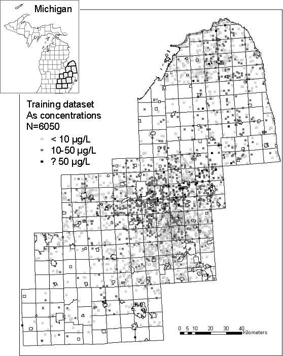
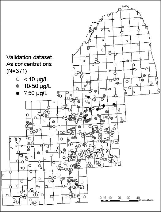
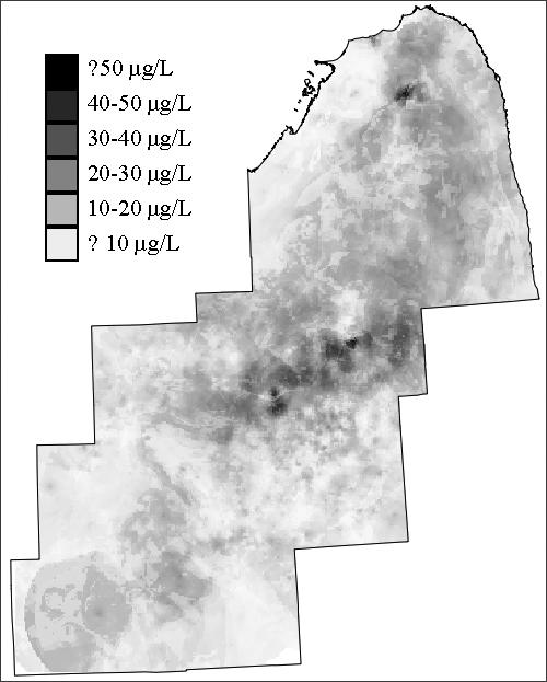
(a): Training dataset of arsenic concentrations in southeastern Michigan used to build predictive spatial models; (b) Validation dataset for testing accuracy of predictive models; (c) Resulting map of estimates from the geostatistical model.
Models for Predicting Arsenic Concentrations in Private Well Water
Geographic Averages in Different Regions
In the 1800s, the US Public Lands Survey designated geographic regions called townships and sections in many States, including Michigan (NRC, 1982). The eleven-county study area of southeastern Michigan was partitioned into 36 square mile (∼95.0 square kilometer) townships, and 1 square mile (∼2.6 square kilometer) sections. Sections were selected as a geographic level of analysis because section-based estimates were calculated in another study of lifetime arsenic exposure (Steinmaus et al., 2003); however, since estimates were not available for every section in the study area (due to data sparsity in rural areas), estimates were also calculated at the township level. For each township and section, the arithmetic mean of arsenic concentration was calculated from the training dataset. Median values were also calculated and produced similar results in the validation analyses; therefore, only results using the arithmetic mean are reported. The number of wells with arsenic values in each township ranged from 0−265, with an average of 28 wells per township. In each section, up to 21 wells were associated with arsenic measurements, but there were no arsenic data for 50% of the sections.
Nearest Neighbor Proxy Wells
In the nearest neighbor approach, the well in the training dataset that was nearest a well in the validation dataset was selected using ArcGIS (version 8.1, ESRI, Redlands, CA) and Hawth's Analysis Tool for ArcGIS (http://www.spatialecology.com/htools/tooldesc.php); the arsenic concentration from the nearest neighbor was then used for the estimate. The distance of the nearest neighbor well to the validation well ranged from < 0.1 km – 8.15 km, with 33% of the proxy wells within 0.5 km and 59% of the proxy wells within 1 km. Averages of all nearest neighbors within 0.5 km were also calculated but produced similar results in the validation analyses; therefore, only results using the first nearest neighbor are reported.
Geostatistical Model
The development of the geostatistical model is described in detail elsewhere (Goovaerts et al. 2005). Briefly, the geostatistical model capitalizes on the spatial correlation between arsenic values to make predictions at unsampled locations. A soft indicator kriging approach was adopted, incorporating the spatial pattern in the arsenic data as well as secondary data such as geographic boundaries of different types of bedrock and unconsolidated geologic formations. A cell-declustering technique was used to account for the uneven sampling of the training dataset (Deutsch and Journel, 1998). In the declustering technique, the study area was divided into rectangular cells, and each observation within a cell was assigned a weight inversely proportional to the number of samples within that cell. The geostatistical model predicts arsenic concentration for 500 × 500 square meter pixels.
Validation Dataset
The models for predicting arsenic concentrations in private wells were validated using samples collected between 2003 and 2006 from 371 private wells of home residences in the study area. Homes were selected based on participation in a population-based bladder cancer case-control study. Case participants were recruited from the Michigan State Cancer Registry and controls were selected using a random digit dialing procedure and frequency matched to the cases by age, race, and gender. Homes of participants served by private well water were included in this dataset, reflecting an estimate of a population-based distribution.
The water sampling and analytic protocols have been described elsewhere (Slotnick et al., 2006). In brief, a water sample was collected prior to any treatment systems either from the home tap, basement, or outside spigot; any hosing was removed prior to sample collection. Water was run for two minutes prior to sample collection and collected directly into acid-washed 60 ml low-density polyethylene (LDPE) bottles. Samples were stored on ice in transit, acidified with 100 μL trace-metal grade HNO3 (Fisher Chemical) in the lab, and refrigerated until analysis. One field blank and replicate were collected each day for quality control purposes, resulting in blanks and replicates for 15% of the drinking water samples analyzed. Samples were analyzed for total arsenic at the University of Michigan, School of Public Health by ICP-MS (Agilent Technologies Model 7500c). Prior reports using these data have indicated high reproducibility and minimal measurement error (Slotnick et al., 2006). The average MDL for arsenic was calculated as 0.02 μg/L (n=17); a value of one-half the average MDL (0.01 μg/L) was assigned for water samples below detection limit.
Statistical Analyses
The validation dataset was compared with arsenic concentrations generated by the predictive models. Agreement between predicted and measured concentrations was analyzed using both continuous and categorical scales.
On the continuous scale, Pearson (r) and Spearman rank (ρ) correlation coefficients were calculated between measured and predicted arsenic concentrations using Statistical Package for Social Science (version 10.1; SPSS, Inc., Chicago, IL). Scatter-plots were constructed to display the degree of over- and under-estimation associated with the different models. Spatial autocorrelation was examined in the residuals of the predictive models to assess whether any spatial pattern remained in the error terms. Moran's I analysis using five nearest neighbors was conducted using Space Time Intelligence System (Version 1.3; Terraseer, Inc., Crystal Lake, IL).
Agreement between categories of measured and predicted arsenic concentrations was quantified using the weighted kappa statistic (κw), which measures the amount of agreement between two measures beyond that expected by chance (Szklo and Nieto, 2000). Arsenic concentrations were categorized a priori to reflect cut-offs commonly used in epidemiologic studies of low-to-moderate arsenic levels in drinking water: < 5.00 μg/L, 5.00−9.99 μg/L, 10.0−19.99 μg/L, and ≥ 20.00 μg/L. Weighted kappa values and their 95% confidence intervals were calculated with Statistical Analysis System (version 8.0; SAS Institute, Inc., Cary, NC). Full weight (1.00) was assigned for perfect agreement between categories for measured and predicted arsenic values. A weight of 0.75 was assigned for disagreement between adjacent categories, a weight of 0.5 for disagreement across two categories, and a weight of 0.25 for disagreement across three categories.
Arsenic data were also categorized dichotomously using the US MCL (10 μg/L) as the cut-off value. Measures of sensitivity, specificity, positive predictive value (PPV), negative predictive value (NPV), and percent agreement were calculated for the different models. Sensitivity is defined as the proportion of wells predicted by the models to contain arsenic ≥ 10 μg/L, among those measured in the validation dataset with ≥ 10 μg/L arsenic. Specificity is defined as the proportion of wells predicted to contain arsenic < 10 μg/L, among those measured with < 10 μg/L arsenic. PPV is defined as the proportion of wells measured with arsenic ≥ 10 μg/L, among those predicted to contain ≥ 10 μg/L arsenic. NPV is defined as the proportion of wells measured with arsenic < 10 μg/L, among those predicted to contain < 10 μg/L arsenic.
RESULTS
The training dataset used to construct the predictive models has an arithmetic mean arsenic concentration of 11.89 μg/L, and a median of 4.65 μg/L (Table 1). The arsenic concentrations in the validation dataset are lower, with a mean of 7.69 μg/L and median equal to 2.30 μg/L. The training and validation datasets display similar geographic distribution, with elevated concentrations most frequently located toward the center of the study area, and lower concentrations on the outer parts of the area (Figures 1a and 1b). The map generated by the geostatistical model also reflects this spatial pattern (Figure 1c).
Table 1.
Summary Statistics of Training and Validation Datasets
| Number of Samples | Years Collected | Arithmetic Mean (μg/L) | Median (μg/L) | 10th Percentile (μg/L) | 90th Percentile (μg/L) | |
|---|---|---|---|---|---|---|
| Training Dataset | 6,050 | 1993−2002 | 11.89 | 4.65 | 0.50 | 32.30 |
| Validation Dataset | 371 | 2003−2006 | 7.69 | 2.30 | 0.12 | 22.73 |
Training dataset used to develop predictive models. Validation dataset used to validate predictive models.
For all four models, the predicted values were significantly correlated with the concentrations measured in the validation wells (p<0.001) (Figure 2). The geostatistical model resulted in the highest correlation with Pearson's r = 0.61 and Spearman's ρ = 0.46 (Figure 2). The nearest neighbor approach produced r = 0.46 and ρ = 0.35, slightly better than the predictions of the township mean which led to r = 0.41 and ρ = 0.35. The correlation was higher using the section mean, r = 0.50, ρ = 0.42, although not as high as that produced from the geostatistical model. The section mean, however, could only be calculated using a subset of 186 wells. The other validation wells were located in sections that were not in the training dataset, hence no data were available for estimating the section mean in these areas. For this subset of 186 wells, the correlation was still highest using the geostatistical model (r=0.63, ρ = 0.53). Compared with the section mean, the correlation was similar using the nearest neighbor approach (r=0.50, ρ = 0.36) and slightly lower using the township mean (r=0.45, ρ = 0.40).
Figure 2. Scatterplots comparing model predictions with measured arsenic concentrations from the validation dataset (a) Geostatistical Prediction; (b) Nearest Neighbor Prediction; (c) Township Mean Prediction; (d) Section Mean Prediction.
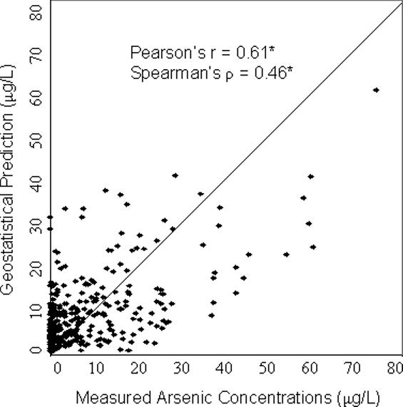
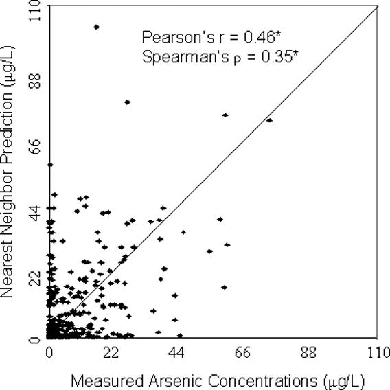
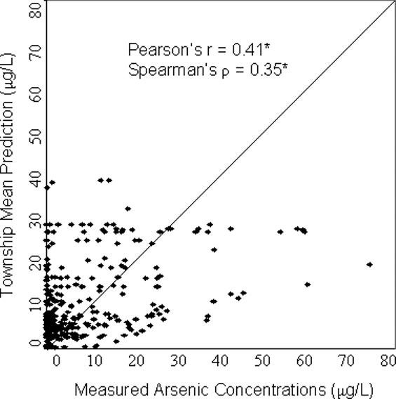
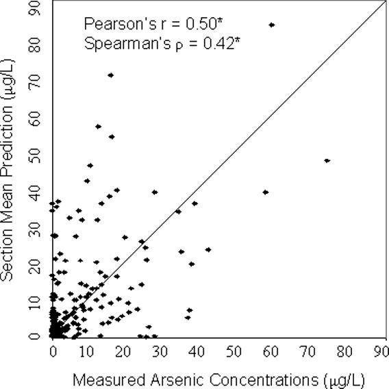
*p<0.001
Significant correlations (p<0.001) were also found when the analysis was conducted on four categories of concentration values defined as the following: <5 μg/L, 5−9.99 μg/L, 10−19.99 μg/L, and ≥20 μg/L (Table 2). In contrast to the correlation analyses on the continuous scale, the nearest neighbor approach generated the strongest agreement between measured and predicted values, as measured by the weighted Kappa statistic: κw = 0.58. For the other approaches, the following values were obtained: for the geostatistical model κw = 0.49, the township mean κw = 0.39, and the section mean κw = 0.54. When these statistics were calculated on the subset of data with section means available (N=186), the agreement remained strongest for the nearest neighbor approach (κw = 0.60), was similar in strength using the geostatistical model (κw = 0.53), and remained lower using the township mean (κw = 0.37).
Table 2.
Comparison of Predicted and Measured Arsenic Concentrations in Validation Dataset Using Four Categories Selected A Priori.
| Measured Arsenic Concentrations (μg/L) | Weighted Kappa | |||||
|---|---|---|---|---|---|---|
| < 5.00 | 5.00−9.99 | 10.00−19.99 | ≥ 20.00 | |||
| Geostatistical Model (N=371) | < 5.00 | 114 | 13 | 13 | 2 | 0.49* |
| 5.00−9.99 | 76 | 14 | 13 | 10 | ||
| 10.00−19.99 | 31 | 15 | 20 | 15 | ||
| ≥ 20.00 | 6 | 2 | 10 | 17 | ||
| Nearest Neighbor Model (N=371) | < 5.00 | 163 | 24 | 18 | 8 | 0.58* |
| 5.00−9.99 | 18 | 11 | 8 | 3 | ||
| 10.00−19.99 | 23 | 7 | 13 | 13 | ||
| ≥ 20.00 | 23 | 2 | 17 | 20 | ||
| Township1 Mean (N=363) | < 5.00 | 85 | 18 | 9 | 2 | 0.39* |
| 5.00−9.99 | 84 | 13 | 17 | 12 | ||
| 10.00−19.99 | 39 | 8 | 11 | 13 | ||
| ≥ 20.00 | 14 | 5 | 17 | 16 | ||
| Section1 Mean (N=186) | < 5.00 | 66 | 11 | 5 | 5 | 0.54* |
| 5.00−9.99 | 17 | 10 | 6 | 5 | ||
| 10.00−19.99 | 12 | 5 | 8 | 3 | ||
| ≥ 20.00 | 10 | 4 | 9 | 10 | ||
p<0.001
Each township occupies approximately 95 km2 and each section approximately 2.6 km2; these geographic regions were designated by the US Public Lands Survey (NRC, 1982). There were 185 wells in which a section mean could not be calculated and 8 wells in which a township mean could not be calculated because arsenic concentrations were not measured in those regions in the training dataset.
Splitting data into two categories using a cut-off of 10 μg/L (the US MCL) resulted in slightly better agreement using both the geostatistical model and nearest neighbor approach compared with the other approaches (Table 3). For these two models, sensitivity ranged from 0.62−0.63, specificity = 0.80, PPV = 0.53, NPV = 0.85, and percent agreement = 75%. In other words, these models are ∼85% accurate at predicting arsenic concentrations below 10 μg/L, and ∼53% accurate at predicting concentrations ≥ μg/L. The models using geographic averages in sections and townships resulted in slightly lower values for all of these measures.
Table 3.
Comparison of Predicted and Measured Arsenic Concentrations in Validation Dataset Using Maximum Contaminant Limit (10 μg/L) as a Threshold.
| Sensitivity | Specificity | Positive Predictive Value (PPV) | Negative Predictive Value (NPV) | Percent Agreement | |
|---|---|---|---|---|---|
| Geostatistical Model | 0.62 (62/100) | 0.80 (217/271) | 0.53 (62/116) | 0.85 (217/255) | 75% |
| Nearest Neighbor Model | 0.63 (63/100) | 0.80 (216/271) | 0.53 (63/118) | 0.85 (216/253) | 75% |
| Township Mean | 0.59 (57/97) | 0.75 (200/266) | 0.47 (57/122) | 0.83 (200/241) | 71% |
| Section Mean | 0.59 (30/51) | 0.77 (104/135) | 0.49 (30/61) | 0.83 (104/125) | 72% |
Sensitivity: Among those wells measured to contain [As] ≥ 10, the proportion of wells predicted to contain [As] ≥ 10.
Specificity: Among those wells measured to contain [As] < 10, the proportion of wells predicted to contain [As] < 10.
PPV: Among those wells predicted to contain [As] ≥ 10, the proportion of wells measured to contain [As] ≥ 10.
NPV: Among those wells predicted to contain [As] < 10, the proportion of wells measured to contain [As] < 10.
The residuals of the geostatistical model and the nearest neighbor approach were examined for spatial pattern and none was detected (Figure 3). Moran's I was not significantly different from zero: Moran's I = 0.019 (p = 0.18) for the residuals of the geostatistical model, and Moran's I = −0.012 (p = 0.34) for the residuals of the nearest neighbor approach. Therefore, remaining variability in the data was not likely to be captured using additional spatial modeling techniques. In addition, the close proximity of wells with both positive and negative residuals (Figure 3) indicates substantial variation in arsenic concentrations over short distances.
Figure 3. Prediction errors for geostatistical model and nearest neighbor approach.
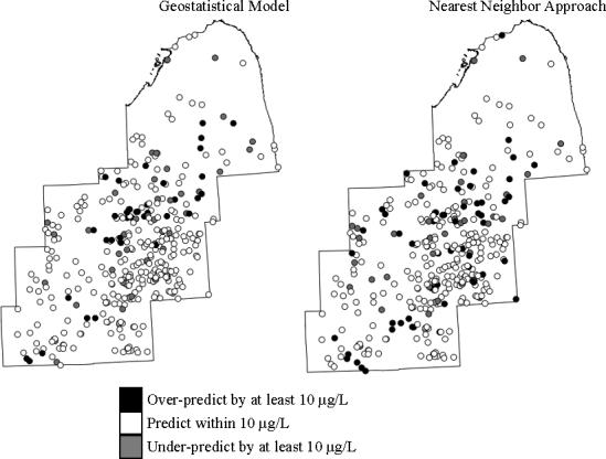
Moran's I analyses specifying five nearest neighbors did not reveal spatial autocorrelation in the residuals of either model (See text).
DISCUSSION
Our study is the first to compare different spatial models of arsenic concentrations in private well water. As monitoring of groundwater for arsenic continues worldwide, a growing number of regions are being identified as having elevated concentrations. Effective models for predicting arsenic concentrations in private well water are critical for identifying high-risk regions and for improving exposure assessment in environmental epidemiologic studies. We assessed model validity using an independent validation dataset of 371 private wells. The spatial models include those commonly applied to predict arsenic: a geostatistical model, a nearest neighbor approach, and arithmetic averages in US Public Lands Survey-defined townships and sections (Bates et al., 2004; Chen et al., 1995; Chen et al., 2003; Chen et al., 2004; Goovaerts et al., 2005; Hassan et al., 2003; Serre et al., 2003; Steinmaus et al., 2003). These models were built on a rich dataset of 6050 arsenic measurements collected over a ten-year period in southeastern Michigan. All models resulted in significant correlations between measured and predicted concentrations on both continuous and categorical scales. Overall, the geostatistical model and nearest neighbor approach outperformed models based on geographic averages in townships or sections.
Of the different models, the geostatistical approach yielded the strongest correlation coefficient (r=0.61), similar in magnitude to that often reported in validations of biomarkers and food frequency questionnaires (r=0.4−0.7) (Cade et al., 2004; Slotnick and Nriagu, 2006; Willett et al., 1985). The nearest neighbor approach resulted in the highest correlation (κw = 0.58) when data were assigned to discrete classes of concentration classified a priori (<5 μg/L, 5−9.99 μg/L, 10−19.99 μg/L, and ≥20 μg/L); the value of this κw indicates a fair-to-good range of agreement (Szklo and Nieto, 2000). The section mean consistently out-performed the township mean, and performed comparably to the other two approaches; however, only 50% of the wells in the validation dataset could be estimated with the section mean. In areas where the section mean could be calculated, the geostatistical model and nearest neighbor approach performed better, presumably because of greater density in the training dataset in those areas.
The geostatistical model and nearest neighbor approach also performed best in analyses where data were split into two categories (above or below 10 μg/L, the US MCL). These models resulted in a 75% agreement, NPV=0.85, PPV=0.53, sensitivity =0.62−0.63, and specificity=0.80. In comparison, an arsenic regression model built for the New England area resulted in lower sensitivity (0.37) and higher specificity (0.93) using 5 μg/L as the cut-off value (Ayotte et al., 2006). NPV and PPV were not reported in the New England study, but were estimated from the data provided as NPV=0.83, and PPV=0.60, similar to what we report in this paper using a higher cut-off value (10 μg/L).
The approaches compared in this paper rely explicitly on spatial pattern in arsenic concentrations. Alternative approaches are available, such as land-use regression (Ayotte et al., 2006) and Classification and Regression Trees (CART) (Schroder, 2006), in which spatial variables are classified into distinct categories and used to predict a dependent variable (e.g., arsenic) in a-spatial analyses. These approaches fail to explicitly consider the spatial pattern or proximity of the dependent variable, but rather take advantage of regionally available factors, such as geology, land use/cover, and hydrology in making predictions (Ayotte et al., 2006). Factors that vary greatly from well to well, however, such as well depth, are often difficult to estimate at unsampled locations, and therefore challenging to include in these predictive models. The geostatistical model presented in our analyses incorporated geologic characteristics in addition to the spatial pattern of the arsenic concentrations. Future research should investigate if a model that accounts for additional hydro-geologic factors along with spatial pattern in arsenic concentrations improves predictive power.
Our analyses are not without limitations. The training dataset was collected under a preferential sampling scheme in which individuals concerned about high levels of arsenic requested tests of their well water. The validation dataset was collected under a sampling protocol that approximated the population density of the study area. This difference in sampling protocols resulted in a higher average arsenic concentration in the training dataset compared with the validation dataset (Table 1). Nonetheless, wells were not consistently over-predicted; in fact, the close proximity of wells with both over- and under-predicted arsenic concentrations (Figure 3) suggests limited consequences from using this preferentially sampled training dataset. This was true whether or not a declustering procedure was adopted to adjust for the preferential sampling, as was the case with the geostatistical approach.
The validation dataset was collected from 2003−2006, whereas the training dataset was collected from 1993−2002. If temporal variability exists in arsenic concentrations in well water, this could explain some of the differences between predicted and measured concentrations. However, temporal analyses of arsenic in wells sampled 6−23 months apart revealed little variability in southeastern Michigan (r=0.91) (Slotnick et al., 2006), consistent with reports of limited temporal variability from other regions (Cheng et al., 2005; Steinmaus et al., 2005). Nevertheless, an implicit assumption in the use of these spatial models is that arsenic concentrations in private wells remain relatively stable over time. Reliable long-term datasets have yet to be identified for verifying this assumption. Given our findings, the high degree of spatial variability within each 95 km2 township likely contributes to the error in the township mean estimate. Using the smaller spatial scale of a section (∼2.6 km2), the estimate improved, but a section mean was only capable of being calculated for 50% of the wells in the validation dataset. The nearest neighbor approach used an even smaller spatial scale, with 33% of the wells within 0.5 km of the nearest neighbor predictor, and resulted in better performance. Furthermore, the estimate was not constrained by artificial administrative boundaries. The geostatistical model, on the other hand, took advantage of small scale, medium scale, and large scale spatial correlation, but produced an estimate no better than the nearest neighbor approach, which used only small-scale variability. This was surprising given that the geostatistical model also accounted for bedrock and unconsolidated geologic boundaries. The large nugget effect (Goovaerts et al., 2005) and extreme variability in well water arsenic concentrations (Smedley and Kinniburgh, 2002) may help to explain why these models performed similarly.
The spatial models of arsenic concentrations in private well water presented herein are being examined for use in an assessment of exposure to arsenic in drinking water at past residences in an ongoing bladder cancer case-control study in southeastern Michigan. From an epidemiologic perspective, the predictive power reported here is better than that often reported for nutritional and environmental biomarkers or food frequency questionnaires. In addition, the misclassification is likely to be nondifferential as the predictive model will be applied to past residences of both cases and controls. There are several features of the geostatistical model that may prove useful for epidemiologic analyses. If researchers are interested in quantifying exposure misclassification, the geostatistical approach produces a map of variance associated with the prediction estimate. This variance could then be explored in logistic regression analyses to assess the effect of misclassification on the results. In addition, the flexibility of the geostatistical approach to incorporate spatial pattern along with geologic/hydrologic characteristics could enable future improvements in the modeling approach.
Individual lifetime exposure to arsenic in drinking water is best estimated through direct measurement at each drinking water source. Unfortunately, direct measurement at major locations over the life-course is impossible because of (1) cost considerations and (2) wells that no longer exist. For these reasons, models for predicting arsenic concentrations in private well water are necessary. These results indicate that the geostatistical model and nearest neighbor approach were the superior spatial models in predicting arsenic concentrations in southeastern Michigan groundwater. However, similar validation analyses should be conducted in other regions to appreciate how widely these findings may be generalized since the processes responsible for arsenic mobilization differ from one place to another.
ACKNOWLEDGMENTS
We would like to thank the participants of this study for taking part in this research. We would also like to thank Stacey Fedewa, Aaron Linder, Nicholas Mank, Caitlyn Meservey, and Taylor Builee for valuable assistance with data collection and laboratory analyses. We are grateful to the Michigan State Cancer Registry and the Michigan Public Health Institute for assisting with participant recruitment. This research was funded by the National Cancer Institute, grant R01 CA96002-10.
Footnotes
Publisher's Disclaimer: This is a PDF file of an unedited manuscript that has been accepted for publication. As a service to our customers we are providing this early version of the manuscript. The manuscript will undergo copyediting, typesetting, and review of the resulting proof before it is published in its final citable form. Please note that during the production process errors may be discovered which could affect the content, and all legal disclaimers that apply to the journal pertain.
REFERENCES
- Ayotte JD, Nolan BT, Nuckols JR, Cantor KP, Robinson GR, Jr., Baris D, Hayes L, Karagas M, Bress W, Silverman DT, Lubin J. Modeling the probability of arsenic in groundwater in New England as a tool for exposure assessment. Environ. Sci. Technol. 2006;40:3578–3585. doi: 10.1021/es051972f. [DOI] [PubMed] [Google Scholar]
- Bates MN, Rey OA, Biggs ML, Hopenhayn C, Moore LE, Kalman D, Steinmaus C, Smith AH. Case-control study of bladder cancer and exposure to arsenic in drinking water in Argentina. Am. J. Epidemiol. 2004;159:381–389. doi: 10.1093/aje/kwh054. [DOI] [PubMed] [Google Scholar]
- Cade JE, Burley VJ, Warm DL, Thompson RL, Margetts BM. Food-frequency questionnaires: a review of their design, validation and utilisation. Nutr. Res. Rev. 2004;17:5–22. doi: 10.1079/NRR200370. [DOI] [PubMed] [Google Scholar]
- Chen CJ, Hsueh YM, Lai MS. Increased prevalence of hypertension and long-term arsenic exposure. Hypertension. 1995;25:53–60. [PubMed] [Google Scholar]
- Chen CL, Hsu LI, Chiou HY, Hsueh YM, Chen SY, Wu MM, Chen CJ. Ingested arsenic, cigarette smoking, and lung cancer risk: a follow-up study in arseniasis-endemic areas in Taiwan. JAMA. 2004;292:2984–2990. doi: 10.1001/jama.292.24.2984. [DOI] [PubMed] [Google Scholar]
- Chen YC, Su HJJ, Guo YLL, Hsueh YM, Smith TJ, Ryan LM, Lee MS, Christiani DC. Arsenic methylation and bladder cancer risk in Taiwan. Cancer Cause. Control. 2003;14:303–310. doi: 10.1023/a:1023905900171. [DOI] [PubMed] [Google Scholar]
- Cheng Z, Van Geen A, Seddique AA, Ahmed KM. Limited temporal variability of arsenic concentrations in 20 wells monitored for 3 years in Araihazar, Bangladesh. Environ. Sci. Technol. 2005;39:4759–4766. doi: 10.1021/es048065f. [DOI] [PubMed] [Google Scholar]
- Chiou HY, Huang WI, Su CL, Chang SF, Hsu YH, Chen CJ. Dose-response relationship between prevalence of cerebrovascular disease and ingested inorganic arsenic. Stroke. 1997;28:1717–1723. doi: 10.1161/01.str.28.9.1717. [DOI] [PubMed] [Google Scholar]
- Deutsch CV, Journel AG. GSLIB: Geostatistical Software Library and User's Guide. 2nd edition Oxford Univ. Press; New York, NY, USA: 1998. [Google Scholar]
- Ford RG, Fendorf S, Wilkin RT. Introduction: Controls on arsenic transport in near-surface aquatic systems. Chem. Geol. 2006;228:1–5. [Google Scholar]
- Goovaerts P, AvRuskin G, Meliker J, Slotnick M, Jacquez G, Nriagu J. Geostatistical modeling of the spatial variability of arsenic in groundwater of southeast Michigan. Water Resour. Res. 2005;41:W07013. [Google Scholar]
- Haack SK, Treccani SL. Water Resources Investigation Report 00−4171. US Geological Survey; Reston, VA, USA: 2000. Arsenic concentration and selected geochemical characteristics for ground water and aquifer materials in southeastern Michigan. [Google Scholar]
- Harvey CF, Ashfaque KN, Yu W, Badruzzaman ABM, Ali MA, Oates PM, Michael HA, Neumann RB, Beckie R, Islam S, Ahmed MF. Groundwater dynamics and arsenic contamination in Bangladesh. Chem. Geol. 2006;228:112–136. [Google Scholar]
- Hassan MM, Atkins PJ, Dunn CE. The spatial pattern of risk from arsenic poisoning: a Bangladesh case study. J. Environ. Sci. Health A. 2003;38:1–24. doi: 10.1081/ese-120016590. [DOI] [PubMed] [Google Scholar]
- Hopenhayn-Rich C, Browning SR, Hertz-Picciotto I, Ferreccio C, Peralta C, Gibb H. Chronic arsenic exposure and risk of infant mortality in two areas of Chile. Environ. Health Perspect. 2000;108:667–673. doi: 10.1289/ehp.00108667. [DOI] [PMC free article] [PubMed] [Google Scholar]
- Kim MJ, Nriagu J, Haack S. Arsenic species and chemistry in groundwater of southeast Michigan. Environ. Pollut. 2002;120:379–390. doi: 10.1016/s0269-7491(02)00114-8. [DOI] [PubMed] [Google Scholar]
- Mazumder DNG, Steinmaus C, Bhattacharya P, von Ehrenstein OS, Ghosh N, Gotway M, Sil A, Balmes JR, Haque R, Hira-Smith MM, Smith AH. Bronchiectasis in persons with skin lesions resulting from arsenic in drinking water. Epidemiology. 2005;16:760–765. doi: 10.1097/01.ede.0000181637.10978.e6. [DOI] [PubMed] [Google Scholar]
- Meliker JR, Slotnick MJ, AvRuskin GA, Kaufmann A, Fedewa SA, Goovaerts P, Jacquez GM, Nriagu JO. Individual lifetime exposure to inorganic arsenic using a Space-Time Information System. Int. Arch. Occup. Environ. Health. 2007;80:184–197. doi: 10.1007/s00420-006-0119-2. [DOI] [PubMed] [Google Scholar]
- MDPH (Michigan Department of Public Health) Division of Environmental Epidemiology, Michigan Department of Public Health. Lansing, MI, USA: 1982. Arsenic in drinking water -- A study of exposure and clinical survey. [Google Scholar]
- NRC . Modernization of the Public Land Survey System. National Academy of Sciences Press; Washington, D.C.: 1982. [Google Scholar]
- Rahman M, Tondel M, Ahmad SA, Axelson O. Diabetes mellitus associated with arsenic exposure in Bangladesh. Am. J. Epidemiol. 1998;148:198–203. doi: 10.1093/oxfordjournals.aje.a009624. [DOI] [PubMed] [Google Scholar]
- Rahman M, Vahter M, Sohel N, Yunus M, Wahed MA, Streatfield PK, Ekstrom E-C, Persson LA. Arsenic exposure and age- and sex-specific risk for skin lesions: a population-based case-referent study in Bangladesh. Environ. Health Perspect. 2006;114:1847–1852. doi: 10.1289/ehp.9207. [DOI] [PMC free article] [PubMed] [Google Scholar]
- Peters SC, Blum JD, Klaue B, Karagas MR. Arsenic occurrence in New Hampshire drinking water. Environ. Sci. Technol. 1999;33:1328–1333. [Google Scholar]
- Schroder W. GIS, geostatistics, metadata banking, and tree-based models for data analysis and mapping in environmental monitoring and epidemiology. Int. J. Med. Microbiol. 2006;296(S1):23–36. doi: 10.1016/j.ijmm.2006.02.015. [DOI] [PubMed] [Google Scholar]
- Serre ML, Kolovos A, Christakos G, Modis K. An application of the holistochastic human exposure methodology to naturally occurring arsenic in Bangladesh drinking water. Risk Anal. 2003;23:515–528. doi: 10.1111/1539-6924.t01-1-00332. [DOI] [PubMed] [Google Scholar]
- Slotnick MJ, Meliker JR, Nriagu JO. Effects of Time and Point-of-Use Devices on Arsenic Levels in Southeastern Michigan Drinking Water, USA. Sci. Tot. Environ. 2006;369:42–50. doi: 10.1016/j.scitotenv.2006.04.021. [DOI] [PubMed] [Google Scholar]
- Slotnick MJ, Nriagu JO. Validity of human nails as a biomarker of arsenic and selenium exposure: A review. Environ. Res. 2006;102:125–139. doi: 10.1016/j.envres.2005.12.001. [DOI] [PubMed] [Google Scholar]
- Smedley PL, Kinniburgh DG. A review of the source, behavior and distribution of arsenic in natural waters. Appl. Geochem. 2002;17:517–568. [Google Scholar]
- Steinmaus C, Yuan Y, Bates MN, Smith AH. Case-control study of bladder cancer and drinking water arsenic in the western United States. Am. J. Epidemiol. 2003;158,:1193–1201. doi: 10.1093/aje/kwg281. [DOI] [PubMed] [Google Scholar]
- Steinmaus C, Yuan Y, Smith AH. The temporal stability of arsenic concentrations in well water in western Nevada. Environ. Res. 2005;99:164–168. doi: 10.1016/j.envres.2004.10.003. [DOI] [PubMed] [Google Scholar]
- Szklo M, Nieto FJ. Epidemiology: Beyond the basics. Aspen Publishers; Gaithersburg, MD, USA: 2000. [Google Scholar]
- Tseng CH. Effects and dose-response relationships of skin cancer and blackfoot disease with arsenic. Environ. Health Perspect. 1977;19:109–19. doi: 10.1289/ehp.7719109. [DOI] [PMC free article] [PubMed] [Google Scholar]
- Van Geen A, Zheng Y, Versteeg R, Stute M, Horneman A, Dhar R, Steckler M, Gelman A, Small C, Assan H, Graziano JC, Hussein I, Ahmed KM. Spatial variability of arsenic in 6000 tube wells in a 25 km2 area of Bangladesh. Water Resour. Res. 2003;39:1140–1155. [Google Scholar]
- Van Geen A, Zheng Y, Cheng Z, Aziz Z, Horneman A, Dhar RK, Mailloux B, Stute M, Weinman B, Goodbred S, Seddique AA, Hoque MA, Ahmed KM. A transect of groundwater and sediment properties in Araihazar, Bangladesh: Further evidence of decoupling between As and Fe mobilization. Chem. Geol. 2006;228:85–96. [Google Scholar]
- Wasserman GA, Liu X, Parvez F, Ahsan H, Factor-Litvak P, van Green A, Slavkovich V, Lolacono NJ, Cheng Z, Hussain I, Momotaj H, Graziano JH. Water arsenic exposure and children's intellectual function in Araihazar, Bangladesh. Environ. Health Perspect. 2004;112:1329–1333. doi: 10.1289/ehp.6964. [DOI] [PMC free article] [PubMed] [Google Scholar]
- Willett WC, Sampson L, Stampfer MJ, Rosner B, Bain C, Witschi J, Hennekens CH, Speizer FE. Reproducibility and validity of a semiquantitative food frequency questionnaire. Am. J. Epidemiol. 1985;122,:51–65. doi: 10.1093/oxfordjournals.aje.a114086. [DOI] [PubMed] [Google Scholar]
- Yang CY, Chang CC, Tsai SS, Chuang HY, Ho CK, Wu TN. Arsenic in drinking water and adverse pregnancy outcome in an arseniasis-endemic area in northeastern Taiwan. Environ. Res. 2003;91:29–34. doi: 10.1016/s0013-9351(02)00015-4. [DOI] [PubMed] [Google Scholar]