Estimating neurotransmitter kinetics with ntPET: A simulation study of temporal precision and effects of biased data

Abstract

We recently introduced ntPET (neurotransmitter PET), an analysis technique which estimates the kinetics of stimulus-induced neurotransmitter (NT) release. Here, we evaluate two formulations of ntPET. The arterial (ART) approach measures the tracer input function (TIF) directly. The reference (REF) approach derives the TIF from reference region data. Arterial sampling is considered the gold standard in PET modeling but reference region approaches are preferred for reduced cost and complexity. If simulated PET data with unbiased TIFs were analyzed using ART or REF, temporal precision was better than three minutes provided NT concentration peaked less than 30 minutes into the scanning session. The consequences of biased TIFs or stimulus-induced changes in tracer delivery were also evaluated. ART TIFs were biased by the presence of uncorrected radiometabolites in the plasma whereas REF TIFs were biased by specific binding in the reference region. Simulated changes in tracer delivery emulated ethanol-induced blood flow alterations observed previously with PET (Volkow et al., 1988). ART performance deteriorated significantly if metabolites amounted to 50% of plasma radioactivity by 60 minutes. The accuracy and precision of REF were preserved even if the reference region contained 40% of the receptor density of the target region. Both methods were insensitive to blood flow alterations (proportional changes in K₁ and k₂). Our results suggest that PET data contain information – heretofore not extracted – about the timing of NT release. The REF formulation of ntPET proved to be robust to many plausible model violations and under most circumstances is an appropriate alternative to ART.

INTRODUCTION

Researchers have used PET and SPECT to detect acute changes in endogenous neurotransmitter (NT) concentration by its displacement of receptor ligand tracers. PET and SPECT studies have detected NT release in response to pharmacological challenges, including amphetamine (e.g., Dewey et al., 1993; Innis et al., 1992; Laruelle et al., 1995; Mach et al., 1997), cocaine (Mach et al., 1997; Volkow et al., 1999), methylphenidate (Mach et al., 1997; Spencer et al., 2006; Volkow et al., 1999; Volkow et al., 1994) and other drugs, as well as behavioral challenges such as videogaming (Koepp et al., 1998), gambling and monetary reward (Pappata et al., 2002; Zald et al., 2004), and other tasks. In conventional PET analyses, NT release is detected by change in binding potential (BP: e.g., Logan et al., 1996; Logan et al., 1990), an index of the time-averaged decrease in receptor availability from baseline to activation condition. Novel methods to detect changes in NT concentration have been proposed (Alpert et al., 2003; Aston et al., 2000; Friston et al., 1997; Pappata et al., 2002; Zhou et al., 2006), but these techniques, like change in BP, provide limited or no information about the timing of NT release. To recover potentially important variations in the timing of neurotransmitter fluctuations, we have developed neurotransmitter PET (ntPET), a modeling and parameter estimation method which characterizes the temporal profile of NT release by combining PET data from rest (constant NT) and activation (time-varying NT) conditions and fitting them simultaneously (Morris et al., 2005).

PET and SPECT studies have revealed the in vivo spatial distribution of various neuroreceptors and transporters and their possible implications in pathological states such as schizophrenia (Buchsbaum et al., 2006; Talvik et al., 2003), alcoholism (Heinz et al., 1998; Szabo et al., 2004), and epilepsy (Fedi et al., 2006; Picard et al., 2006). However, the time course of neurotransmitter release in response to specific stimuli has not been measured in humans and may encode pertinent information about brain function. It has been hypothesized that the speed of dopamine release elicited by a drug may be a strong indicator of the drug’s addictive liability and potential for abuse (Spencer et al., 2006; Volkow et al., 1995; Volkow et al., 1999; Volkow and Swanson, 2003). Boileau et al. (2007) speculated that amphetamine-and placebo-induced dopamine responses may follow distinct time courses, but noted that PET was not capable of distinguishing such differences. An imaging-based method for measuring the temporal profile of NT release, with sufficient resolution and accuracy, would constitute a new tool for addressing such speculations and for evaluating drug action more broadly.

Dynamic PET data reflecting the uptake and retention of receptor tracers has been modeled successfully with the two-tissue compartment model (Mintun et al., 1984). In applying the two compartment model to the data, one assumes a constant concentration of any competitor, such as an endogenous NT. More complicated models (Endres et al., 1997; Morris et al., 1995) have been introduced to accommodate time-varying concentrations of endogenous species. With these models, one can predict the effect of a transient increase in NT level on the dynamic PET data. These models necessarily require more parameters than the Mintun model.

To estimate more than the four parameters of the standard model from PET data, some investigators have tried to increase the information content of the data by experimental manipulation of the system. Along these lines, multiple injections of tracer at different specific activities have been administered during a single scan session (Christian et al., 2004; Delforge et al., 1989, 1990; Huang et al., 1989; Millet et al., 2000; Morris et al., 1996a; Morris et al., 1996b; Muzic et al., 1996). Multiple injection approaches facilitate observation of the system at multiple operating points; model fitting of all the data simultaneously leads to improved identifiability of parameters. Our implementation of ntPET can be seen as an extension of the multiple injection concept to a two scan protocol in which we manipulate the neurotransmitter concentration through pharmacological or cognitive stimulation rather than the concentration of unlabeled tracer. The system is observed in the rest state during one scan and in activation during the other. Data from both scan conditions are analyzed simultaneously. The parameters that describe the uptake and retention of tracer (Θ_TR) and the parameters that describe the profile of NT release in the activation condition (Θ_NT) are estimated concurrently.

In previous PET data analyses, the use of penalty functions has been demonstrated to improve the precision of estimated parameters at the expense of increased bias (Bertoldo et al., 2004; O’Sullivan and Saha, 1999; Zhou et al., 2001; Zhou et al., 2002). Under certain conditions, constrained optimization can yield parameter estimates which minimize the objective function but fit the data poorly (Muzic and Christian, 2006). The ntPET approach, however, uses penalty terms based on prior experimental information in order to promote robust performance.

All compartmental models are driven by one or more input functions. There are two common methods for obtaining the tracer input function (TIF) for PET modeling. One is to obtain arterial blood samples, which can be processed to measure the tracer concentration in arterial plasma. The other is to formulate the TIF in terms of PET data acquired in a reference region that has negligible receptor density (Blomqvist et al., 1990; Cunningham et al., 1991). Arterial sampling is believed to yield an accurate measurement of the TIF and is considered the gold standard in PET modeling, but surgical cannulation of an artery and processing of blood samples can be quite burdensome. Reference region approaches simplify the protocol and reduce costs, although they introduce additional model assumptions. We have developed two variants of ntPET: one which measures the TIF from arterial blood samples (the ART method) and another which derives the TIF from reference region data (the REF method).

All models make assumptions, either explicitly or implicitly. PET models implicitly assume that the TIF is accurately measured. Incorrectly measured input functions may increase the bias and/or variance of estimated parameters. Activation paradigms are known to change regional cerebral blood flow to the brain regions that respond to the stimulus – indeed, this is the underlying principle in functional neuroimaging based on the blood oxygenation level-dependent (BOLD) effect (Kwong et al., 1991; Ogawa et al., 1990). However, changes in blood flow might confound models which assume that flow to the region of interest is constant during the scan. More generally, models with constant coefficients assume that the physiological parameters are constant throughout the study. Many model assumptions are not completely satisfied in practice, so we sought to quantify the impact of likely violations on the estimation of NT profiles.

In this paper, we examine the consequences of model violations on the precision and accuracy of the NT profiles estimated by ntPET from realistic simulated PET data. In particular, we studied the effect of biased TIFs and activation-induced changes in blood flow. The ART and REF variants of ntPET derive their respective TIFs from different measurements, so the relevant model violations that we investigated were necessarily different. To test the robustness of the ART method, we supplied it with arterial plasma curves that were not corrected for the presence of labeled polar metabolites. To test the REF method, we provided it with PET data from non-ideal reference regions that contained receptors. To test the effects of activation-induced changes in tracer delivery, we analyzed simulations of NT release accompanied by blood flow changes and also simulations of flow changes alone. The precise nature of activation-induced alteration of tracer delivery and its impact on blood flow parameters (i.e., K₁ and k₂) remains unclear (Alpert et al., 2003; Logan et al., 1994; Pappata et al., 2002), so multiple scenarios were examined. Based on our results, we offer recommendations on the practical application of the ART and REF formulations of ntPET, including the conditions under which the REF method could serve as an acceptable substitute for the more demanding, but perhaps more accurate, ART method.

METHODS

A. Model Development

The compartmental model used in ntPET (Morris et al., 1995), illustrated schematically in Figure 1, is an extension of the standard two-tissue compartment model to include competition between the tracer and an endogenous NT at the receptor sites. Competitive binding is assumed because both tracer and NT bind specifically to receptors that are present in finite number. The model is comprised of coupled mass balances for the tracer and the NT. The tracer can exist in three possible states (suspended in plasma, C_P(t); free in tissue, F(t); and bound to a receptor, B(t)), whereas the NT can exist as either free (F^NT(t)) or bound (B^NT(t)). The model rate constants represent the rate of transfer of a molecule between states. The rate constants are typically first order, although transition from the free state to the bound state is a bimolecular (and saturable) interaction between free ligand (i.e., tracer or NT) and available (i.e., unoccupied) receptor. The mass balance for free tracer, F(t), is

Figure 1.

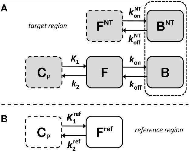
Schematic representation of the enhanced receptor model used by ntPET. A. Tracer can exist in plasma (C_P), free (F), and bound (B) states. Neurotransmitter can be in either the free (F^NT) or bound (B^NT) states. The dotted box around the bound compartments represents the coupling of the states by competition between tracer and neurotransmitter at receptor sites, which exist in limited number. B. Compartmental model for an ideal reference region, which can be used to approximate the plasma input function.

$$\frac{dF(t)}{dt}=K_1{C}_P\hspace{0.17em}(t)-k_2\hspace{0.17em}F(t)-k_{\mathit{on}}\hspace{0.17em}[B_{\max }-B(t)-B^{NT}(t)]\hspace{0.17em}F(t)+k_{\mathit{off}}\hspace{0.17em}B(t)$$ (1)

where B_max is total receptor concentration, including receptors occupied by the NT. In the past, B_max was often used imprecisely to refer to the density of unoccupied receptors. However, the concentration of available receptors is more properly designated B_avail (Innis et al., 2007). The mass balance equation for bound tracer, B(t), is

$$\frac{dB(t)}{dt}=k_{\mathit{on}}\hspace{0.17em}[B_{\max }-B(t)-B^{NT}(t)]\hspace{0.17em}F(t)-k_{\mathit{off}}\hspace{0.17em}B(t)$$ (2)

and the balance for bound NT, B^NT(t), is

$$\frac{d{B}^{NT}(t)}{dt}=k_{\mathit{on}}^{NT}\hspace{0.17em}[B_{\max }-B(t)-B^{NT}(t)]\hspace{0.17em}{F}^{NT}(t)-k_{\mathit{off}}^{NT}\hspace{0.17em}{B}^{NT}(t).$$ (3)

The tracer and neurotransmitter generally do not demonstrate identical binding kinetics, therefore their respective association (k_on, ${\mathrm{k}}_{\mathrm{on}}^{\mathrm{NT}}$) and dissociation (k_off, ${\mathrm{K}}_{\mathrm{off}}^{\mathrm{NT}}$) rate constants are not the same. The state variables in Eq 1-3 have units of chemical concentration.

The output equation relates the compartment concentrations to the PET signal. The PET signal for a given time frame is the sum of the radioactive tracer states weighted by their respective volume fractions, integrated over the frame duration.

$${\mathit{PET}}_i=\frac{1}{\mathrm{\Delta }{t}_i}\underset{t_i-\frac{\mathrm{\Delta }{t}_i}{2}}{\overset{t_i+\frac{\mathrm{\Delta }{t}_i}{2}}{\int }}{\epsilon }_V\hspace{0.17em}{C}_{\mathit{WB}}(t)+{\epsilon }_T\hspace{0.17em}[F(t)+B(t)]\hspace{0.17em}\mathit{SA}(t)dt$$ (4)

The specific activity term, SA(t), converts the free and bound states from molar to radioactivity concentration; SA is time varying due to radioactive decay. The whole blood volume fraction is ε_V and ε_T is the tissue volume fraction, where ε_T=1−ε_V. The midpoint and duration of the i^th frame are t_i and Δt_i, respectively. C_WB(t) is the whole blood radioactivity concentration.

The ntPET model contains two time-varying inputs. The TIF, C_P(t), is the concentration of tracer in the plasma. As mentioned above, the TIF is obtained either by directly sampling arterial blood or by deriving it from PET data in a reference region. The mass balance equation for a reference region (Eq. 1 with binding terms omitted) can be rearranged to yield an expression for C_P(t),

$$C_P(t)=\frac{1}{K_1^{\mathit{REF}}}\hspace{0.17em}\left[\frac{{\mathit{dF}}^{\mathit{REF}}(t)}{\mathit{dt}}+k_2^{\mathit{REF}}{F}^{\mathit{REF}}(t)\right].$$ (5)

Thus, the TIF can be approximated from the time course of the free tracer in the reference region and its time derivative, provided ${\mathrm{K}}_1^{\mathrm{REF}}$ and ${\mathrm{k}}_2^{\mathrm{REF}}$ are estimated with the other model parameters.

The second model input is F^NT(t), the concentration of free NT in the tissue. In the present implementation, the time-varying free NT is parameterized as a gamma variate function,

$$F^{\mathit{NT}}(t)=\mathit{Basal}+\gamma {(t-t_D)}^{\alpha }{e}^{-\beta (t-t_D)}.$$ (6)

Basal is the baseline neurotransmitter concentration prior to perturbation. The magnitude of the response is scaled by γ; the steepness of ascent and descent are dictated by α and β, respectively. The effect of each parameter on the gamma variate function is demonstrated in Figure 2. These NT parameters comprise the elements of the vector Θ_NT. Mathematically, F^NT(t) is an input to the model; physiologically, it is the endpoint that we seek. Since it cannot be measured directly, we must estimate it from the PET data. The timing of the NT response is our primary interest, thus we consider the key characteristics to be delay time, t_D; peak time, t_P = t_D + α/β; and peak height, F^NT(t_P).

Figure 2.

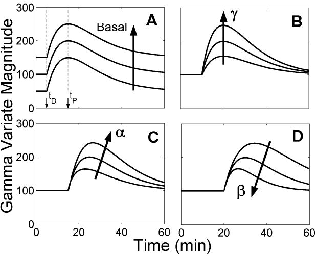
Effect of gamma variate parameters on function output. The impact of delay time, t_D, is demonstrated by incrementing its value between panels. Arrows indicate the progression of the curves as a given parameter increases while all other parameters are held constant. A. Basal affects the scale of the baseline offset but does not influence the magnitude or shape of the transient portion of the curve, which begins at the delay time, t_D. The function reaches a maximum at the peak time, t_P. As t→∞, the curve asymptotically returns to Basal. B. The parameter γ scales the magnitude of the function’s transient phase, but does not change the shape of the curve or the value of the timing parameters, t_D and t_P. C. The parameter α dictates the steepness and duration of the function’s ascent after t_D. D. The parameter β determines the rapidness with which the gamma variate curve returns to Basal. The ratio of α to β controls the time at which the function reaches its maximum value (t_P=t_D+α/β).

The tracer and NT parameters are estimated by simultaneously fitting the model to dynamic PET data acquired during the rest and activation conditions. We assume that tracer parameters are identical in both conditions, whereas the parameters describing NT dynamics are allowed to vary from baseline in the activation condition only.

B. Computer Simulations of PET Data

All programming was done in MATLAB (Mathworks, Inc., Natick, MA); the model was implemented using the COMKAT library of functions (Muzic and Cornelius, 2001). Three different types of data were simulated: (I) noisy TIFs, not biased by model violations, (II) noisy TIFs, biased by model violations, and (III) change in blood flow constant(s) during activation.

I. Unbiased TIFs, No Alteration in Tracer Delivery

A canonical set of tracer parameters (Θ_TR=[K₁, k₂, k_on, k_off, B_max]^T) was chosen to match the cerebral pharmacokinetics of the PET radioligand [¹¹C]raclopride, a dopamine D₂/D₃ receptor antagonist. We targeted a resting BP of approximately 2.0 in creating our simulations. NT parameters (Eq. 6) were selected such that the shape of F^NT(t) resembled the release of dopamine (DA) in response to cocaine (based on (Volkow et al., 1999); see development in (Yoder et al., 2004)), a drug known to cause acute elevation of synaptic DA concentration. The magnitude of F^NT(t) (peak value at 200% of baseline) was chosen to yield a change in BP (see below) less than 0.2, indicative of a modest effect on tracer binding. Simulated delay times ranged, in five minute increments, from five to thirty minutes after raclopride injection. DA association and dissociation rate constants were chosen to agree with in vitro binding data (Fisher et al., 1995). Poisson-like noise was added to the simulated data, with variance

$${\sigma }_i^2={\zeta }^2\frac{{\mathit{PET}}_i}{\mathrm{\Delta }{t}_i}$$ (7)

at the i^th time frame (Landaw and DiStefano, 1984). ζ was chosen to yield a signal-to-noise ratio resembling that of our typical human PET data acquired with raclopride on the ECAT EXACT HR+ (CTI, Knoxville, TN).

For each delay time 25 data sets were generated, each with tracer parameters selected randomly from a ±10% uniform distribution about the canonical parameter set. Thus, 150 data sets (6 different delay times × 25 sets of tracer parameters; see Table 1, lines 1-6) were created. Each data set was generated by solving the ntPET model (Eqs. 1-4) using a standard plasma curve as the TIF (see below) to produce four PET time activity curves (TACs), corresponding to: (1) target region during activation, (2) target region during rest, (3) reference region during activation, and (4) reference region during rest. All simulations of activation were made with a given set of tracer parameters and a time varying NT curve (Eq. 6). All rest TACs were simulated with constant NT (i.e., F^NT(t)=Basal). All unbiased reference region curves were simulated with no receptors (i.e., B_max=0 in reference region).

Table 1.

			True NT Parameters				False Classification Rate
Line #	Case	# Data Sets	tD (min)	α/β (min)	FNT(tP) (% basal)	Measured ΔBP	ART	REF
1	no violations with NT	25	5	10	200	0.155±0.020	0	0
2	no violations with NT	25	10	10	200	0.172±0.026	0	0
3	no violations with NT	25	15	10	200	0.160±0.022	0	0.02
4	no violations with NT	25	20	10	200	0.144±0.023	0	0
5	no violations with NT	25	25	10	200	0.112±0.020	0	0
6	no violations with NT	25	30	10	200	0.093±0.023	0	0
7	no violations null	50	N/A	N/A	0	0.003±0.017	0.04	0.04
8	slow metabolism with NT	25	5	10	200	0.156±0.022	0.08
9	slow metabolism with NT	25	10	10	200	0.164±0.028	0.08
10	slow metabolism with NT	25	15	10	200	0.151±0.018	0
11	slow metabolism with NT	25	20	10	200	0.122±0.024	0
12	slow metabolism with NT	25	25	10	200	0.110±0.022	0
13	slow metabolism with NT	25	30	10	200	0.083±0.023	0
14	slow metabolism null	50	N/A	N/A	0	0.007±0.019	0.22
15	moderate metabolism with NT	25	5	10	200	0.156±0.017	0.04
16	moderate metabolism with NT	25	10	10	200	0.159±0.022	0
17	moderate metabolism with NT	25	15	10	200	0.136±0.020	0
18	moderate metabolism with NT	25	20	10	200	0.127±0.028	0
19	moderate metabolism with NT	25	25	10	200	0.098±0.020	0
20	moderate metabolism with NT	25	30	10	200	0.079±0.016	0
21	moderate metabolism null	50	N/A	N/A	0	0.013±0.020	0.90
22	RDRR:T 1:5 with NT	25	5	10	200	0.154±0.025		0
23	RDRR:T 1:5 with NT	25	10	10	200	0.164±0.017		0
24	RDRR:T 1:5 with NT	25	15	10	200	0.151±0.023		0
25	RDRR:T 1:5 with NT	25	20	10	200	0.126±0.020		0.04
26	RDRR:T 1:5 with NT	25	25	10	200	0.096±0.019		0.04
27	RDRR:T 1:5 with NT	25	30	10	200	0.078±0.020		0
28	RDRR:T 1:5 null	50	N/A	N/A	0	0.009±0.020		0.02
29	RDRR:T 2:5 with NT	25	5	10	200	0.150±0.016		0
30	RDRR:T 2:5 with NT	25	10	10	200	0.159±0.023		0.02
31	RDRR:T 2:5 with NT	25	15	10	200	0.138±0.020		0
32	RDRR:T 2:5 with NT	25	20	10	200	0.113±0.020		0
33	RDRR:T 2:5 with NT	25	25	10	200	0.088±0.018		0
34	RDRR:T 2:5 with NT	25	30	10	200	0.061±0.020		0
35	RDRR:T 2:5 null	50	N/A	N/A	0	-0.005±0.019		0.02
36	↓BFREF with NT	25	15	10	200	0.169±0.027		0
37	↓BFREF null	50	N/A	N/A	0	0.016±0.023		0.10
38	↑BFTAR, ↓BFREF with NT	25	15	10	200	0.167±0.023	0	0
39	↑BFTAR, ↓BFREF null	50	N/A	N/A	0	0.009±0.017	0.04	0.08
40	↓ ${\mathrm{K}}_1^{\mathrm{REF}}$ with NT	25	15	10	200	0.085±0.026		0.24
41	↓ ${\mathrm{K}}_1^{\mathrm{REF}}$ null	50	N/A	N/A	0	-0.074±0.020		0
42	↑K1, ↓ ${\mathrm{K}}_1^{\mathrm{REF}}$ with NT	25	15	10	200	-0.009±0.019	0.12	0.96
43	↑K1, ↓ ${\mathrm{K}}_1^{\mathrm{REF}}$ null	50	N/A	N/A	0	-0.149±0.021	0	0

α/β indicates the latency between time of NT response onset (t_D) and time of NT response peak (t_P=t_D+α/β). Measured ΔBP is the change in binding potential calculated from the simulated time activity curves by graphical analysis with reference region input. False classification rate is the fraction of false positive or false negative events as determined using the 95% confidence threshold obtained from analysis of noisy null data sets with no model violations.

For all simulations, the TIFs were defined according to

$$C_P\hspace{0.17em}(t)=({\beta }_{1}t-{\beta }_2-{\beta }_3)e^{-k_{1}t}+{\beta }_2{e}^{-k_{2}t}+{\beta }_3{e}^{-k_{3}t}$$ (8)

with β₁ = 12 (nM·min^-1), β₂ = 1.8 (nM), β₃ = 0.45 (nM), k₁ = 4 (min^-1), k₂ = 0.5 (min^-1), and k₃ = 0.008 (min^-1) (Feng et al., 1993). Tissue fraction (ε_T) and vascular fraction (ε_V) were fixed at 0.95 and 0.05, respectively. A 60 minute scan was simulated with 60 one minute frames.

Change in binding potential (ΔBP≡[BP_rest−BP_activ]/BP_rest), a conventional index of NT release, was determined for each data set in order to characterize the simulations. Binding potentials were calculated for each pair of simulated target and reference region TACs using a graphical method with a reference region input (Logan et al., 1996). ΔBP was less than 0.2 in all simulations. In agreement with previous findings (Yoder et al., 2004), ΔBP varied with NT timing (see lines 1-6 of Table 1).

Null Data Sets

In order to address the false discovery rate, 50 ‘null’ data sets were generated. A null data set consisted of four TACs, as above, but NT concentration was constant over time in the target region during activation. ΔBP for the null data sets was negligible (see Table 1, line 7), verifying the absence of NT response.

II.a. Biased TIFs: ART Method

To test the ART method, the input function used for simulation of data was subjected to first order metabolism such that unmetabolized (native) tracer accounted for either 80% (slow metabolism), 50% (moderate metabolism), or 10% (fast metabolism) of the total plasma radioactivity at the end of the scan period. The TIF to be used for parameter estimation (i.e., analysis), however, was taken to be the total plasma signal without correction for labeled metabolites. Thus, the input function for ART estimations was a corrupted version of the true TIF. Tracer metabolites were taken to be polar molecules and unable to cross the blood-brain-barrier, so tests of REF, which uses only tissue TACs, did not consider this violation. 450 activation (3 metabolism rates × 6 delay times × 25 tracer parameter sets; see Table 1 lines 8-13, 15-20) and 150 null (3 metabolism rates × 50 tracer parameter sets; see Table 1 lines 14, 21) data sets were generated as described above.

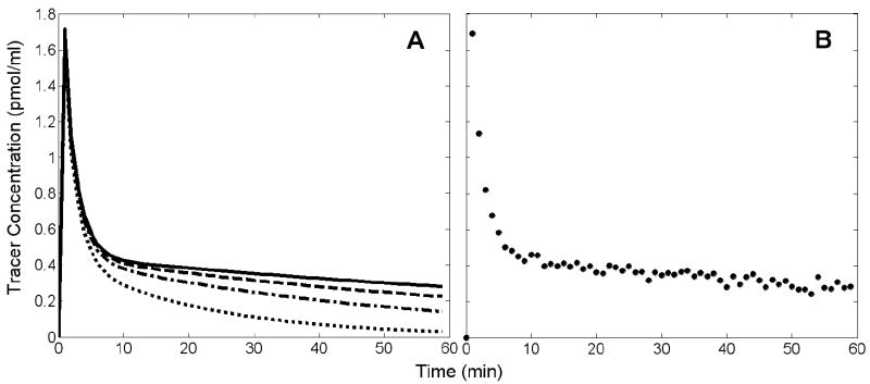
The effect of metabolism on the time course of tracer in the plasma is illustrated in Figure 3. The concentration of native tracer diminishes more quickly with higher rates of metabolism (Figure 3A). The rate of metabolism does not change the total plasma radioactivity, but as metabolism progresses a decreasing proportion of the plasma signal represents native tracer. By not correcting for the accumulation of labeled metabolites we introduced a nonlinear bias to the TIF that increased with scan time and speed of metabolism. Figure 3B shows an example of a noisy, simulated TIF, derived from total plasma radioactivity without correction for metabolites.

Figure 3.

A. Time course of unmetabolized tracer. Solid black curve is a noiseless TIF without metabolism. Other curves represent TIFs with first order metabolism, with rate constants selected such that unmetabolized tracer contributed 80% (dashed), 50% (dashed-dotted), or 10% (dotted) of total plasma radioactivity at 60 min. These TIFs were used for simulation of data when testing ART with biased TIFs. B. Example of a noisy TIF without correction for metabolites, used when performing estimations with ART method. The example TIF is representative of the input used for all ART estimations because the time course of total plasma radioactivity was the same for all cases of simulated tracer metabolism.

For all simulations in this category, ΔBP from data sets with NT release were smaller the more rapid the metabolism. As with data sets having no model violations, ΔBP was less than 0.2 and varied with NT timing (Table 1, lines 8-13 and 15-20). All null data sets had very small ΔBP for all rates of metabolism (see lines 14, 21 in Table 1).

II.b. Biased TIFs: REF Method

Data sets were generated with non-ideal reference regions (i.e., having non-zero receptor density) to test the REF method. Specifically, we considered reference-to-target receptor density ratios (RDR_R:T) of 1:20, 1:10, 1:5, and 2:5. These conditions violated the central assumption of all reference region approaches, namely, that the reference region is devoid of specific binding. ART does not use reference region data, so testing of ART did not consider this violation. NT release during activation was confined to the target region. 600 activation (4 different RDR_R:T × 6 delay times × 25 sets of tracer parameters; see Table 1 lines 22-27, 29-34) and 200 null (4 different RDR_R:T × 50 sets of tracer parameters; see Table 1 lines 28 and 35) data sets were generated as described above.

Figure 4 shows examples of reference region TACs containing specific binding and the TIFs derived from them. Figure 4A confirms that increasing receptor density increases retention of tracer in the reference tissue. Following the initial peak, the scale of the biased TIFs reflects the degree of retention in the reference TACs, as shown in Figure 4B.

Figure 4.

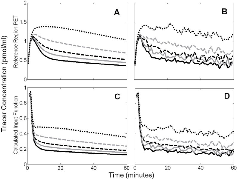
Simulated noiseless (A) and noisy (B) reference region PET data and the TIFs derived from them (C,D). Solid black curves correspond to reference region with no receptors. Other curves represent data with reference-to-target receptor density ratios (RDR_R:T) of 1:20 (solid gray), 1:10 (dashed black), 1:5 (dashed gray), or 2:5 (dotted black).

Tracer binding in the reference region caused a negative bias in BP, as has been noted previously (Asselin et al., 2007; Slifstein et al., 2000). In turn, ΔBP of our simulated data was smaller the greater the reference region receptor density. ΔBP from null data was very small and was not dependent on the amount of reference region binding (see Table 1, lines 28 and 35).

III. Altered Tracer Delivery

Changes in blood flow or initial tracer uptake constants (i.e., K₁ and ${\mathrm{K}}_1^{\mathrm{REF}}$) as a result of activation would constitute a violation of the assumption that kinetic rate constants (i.e., the elements of Θ_TR) are time-invariant. We addressed four possible stimulus-induced alterations of tracer delivery based on the effects of an ethanol challenge (Volkow et al., 1988): (1) decrease in blood flow to the reference region (BF^REF), (2) decrease of ${\mathrm{K}}_1^{\mathrm{REF}}$ by 10%, (3) increase in blood flow to the target region (BF^TAR) concurrent with decreased BF^REF, and (4) increase of K₁ by 10% concurrent with decrease of ${\mathrm{K}}_1^{\mathrm{REF}}$ by 10%. To simulate decreased BF^REF, both ${\mathrm{K}}_1^{\mathrm{REF}}$ and ${\mathrm{k}}_2^{\mathrm{REF}}$ were lowered by 10%. To simulate increased BF^TAR, both K₁ and k₂ were increased by 10%. In each case, alteration of tracer delivery started 15 min after the start of the activation scan and persisted for the remainder of the scan. The change in parameter(s) was implemented by simulating the data in two distinct epochs. First, data were simulated in the conventional manner (i.e., with zero initial conditions) up to the time at which blood flow or K₁ changed. Then, using the state variables from the end of the first epoch as the initial conditions for the second epoch, data were simulated with the blood flow parameter(s) at new, constant value(s) for the remainder of the scan. All four alterations of tracer delivery were simulated both with and without NT response.

Figure 5 shows noiseless examples of simulated TACs containing altered tracer delivery. In Figure 5A, TACs in the rest condition are overlaid on TACs generated with an increase of BF^TAR and a decrease of BF^REF beginning at 15 minutes. For both regions, TACs with changes in blood flow were nearly indistinguishable from TACs from those in the rest condition. In Figure 5B, the same comparison is made for increased K₁ and decreased ${\mathrm{K}}_1^{\mathrm{REF}}$. The change began at 15 minutes and there was no NT response. TACs simulated with changes in K₁ or ${\mathrm{K}}_1^{\mathrm{REF}}$ were shaped differently than those without activation-induced artifact.

Figure 5.

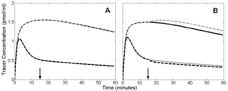
Effect of altered tracer delivery on tissue time activity curves (TACs). Solid black curves and solid gray curves correspond to noiseless, simulated TACs from target and reference region, respectively, during rest condition. Alterations in delivery were simulated by instantaneously changing tracer parameters 15 minutes into activation scan. A. Increased blood flow to target region (dashed gray) and decreased flow to reference region (dashed black). These curves almost completely overlay the TACs from the rest condition. Arrow indicates time at which flow changes occurred. B. Increased K₁ (dashed gray) and decreased ${\mathrm{K}}_1^{\mathrm{REF}}$ (dashed black). Arrow indicates time at which K₁ increased and ${\mathrm{K}}_1^{\mathrm{REF}}$ decreased.

Simulations including changes in blood flow had ΔBP values similar to equivalent simulations without flow artifacts (Table 1, lines 36-39). Simulations with altered K₁ or ${\mathrm{K}}_1^{\mathrm{REF}}$ and NT release were characterized by markedly lower ΔBP (Table 1, lines 40 and 42). Null data sets with altered K₁ or ${\mathrm{K}}_1^{\mathrm{REF}}$ gave negatives values for measured ΔBP (Table 1, lines 41 and 43).

C. Application of ART and REF Methods

I. Parameter Estimation

Parameter estimation was performed using penalized weighted non-linear least squares. The objective function was composed of the weighted residual sum of squares from the rest and activation conditions and two penalty terms. The first penalty term constrained the time of peak NT concentration (t_P=t_D+α/β) during activation. The second penalty constrained binding potential (BP=k_on[B_max-B-B^NT]/k_off) during rest. The penalized objective function was

$$\mathrm{\Phi }({\mathrm{\Theta }}_{\mathit{TR}},{\mathrm{\Theta }}_{\mathit{NT}})=\sum _i{w}_i\hspace{0.17em}{[{\mathit{PET}}_i^{\mathit{meas}}-{\mathit{PET}}_i({\mathrm{\Theta }}_{TR},{\mathrm{\Theta }}_{NT})]}^2+{\tau }_1\hspace{0.17em}[\exp (-\hspace{0.17em}[t_p\hspace{0.17em}({\mathrm{\Theta }}_{NT})-t_L])+\exp (t_P({\mathrm{\Theta }}_{NT})-t_U)]+{\tau }_2\hspace{0.17em}{[{BP}^{\mathit{meas}}-BP\hspace{0.17em}({\mathrm{\Theta }}_{TR},{\mathrm{\Theta }}_{NT})]}^2$$ (9)

where w_i are the weights applied to each residual (set proportional to ${\mathrm{\sigma }}_{\mathrm{i}}^{-2}$), and τ₁ and τ₂ are weights applied to the penalty terms (τ₁ = τ₂ = 60). t_L and t_U are the upper and lower peak time constraints (t_L = 0 min, t_U = 60 min) and Θ_TR and Θ_NT are the vectors of tracer and NT parameters, respectively. For better performance, one could reasonably assume that the NT response is causal and set t_L to the time of stimulus onset, although we did not do that here. BP(Θ_TR, Θ_NT) is calculated from the estimated parameters on each iteration of the fitting procedure, whereas BP^meas is determined independently by a graphical analysis (Logan et al., 1996) of the rest data prior to parameter estimation. Eq. 9 is minimized by parameters which fit the data from both scan conditions, yield a BP near BP^meas, and find NT events which peak during the scan. For clarity, estimated quantities will be indicated by a caret (e.g., t̂_D is the delay time estimated from data; t_D is the true delay time used in simulations).

Noiseless TIFs were used to generate simulated data, but noisy TIFs were used in the estimation process. The noisy TIFs provided to ART for parameter estimation were produced by adding zero-mean Gaussian noise to the total plasma radioactivity signal. The TIFs used for REF analyses were derived (see Eq. 5) from the noisy simulated reference region data.

II. Parameter Identifiability, Goodness of Fit, and Classification

Due to the large number of parameters being estimated, correlation between parameters, and noise in the data, we were wary of possible dependence of our final estimates on the initial parameter guess. As a precaution, we fit each data set 50 times with 50 initial guesses chosen randomly from a uniform distribution across a wide range of parameter values. Refer to Figure 6 for a plot of the 50 NT responses associated with a typical set of 50 initial guesses. Of the estimations that converged for a given data set, the best model fits to the data were determined by a multiple stage goodness of fit selection process based on objective criteria (Morris et al., 2005). In the first step, we eliminated fits with weighted residual sum of squares greater than the median. From the fits that were retained, we kept only the ones having at least as many runs (zero crossings in the residuals) as the median number. Therefore, analysis of each data set yielded multiple answers representing a group of NT responses that best explain the data from both scan conditions (i.e., an “NT profile family”). Reported parameters (i.e., t̂_D, t̂_P, F̂^NT(t̂_P)) for a single data set represent peak height, delay time, and peak time averaged over each member of the resultant NT profile family. Reported standard deviations (see Results) represent the variability in reported parameters from multiple data sets.

Figure 6.

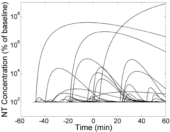
The 50 NT profiles corresponding to a typical set of 50 randomly selected initial guesses used to fit a data set multiple times. The vertical axis is plotted on a logarithmic scale, as the magnitudes of the NT profiles at initial guess are highly variable.

In the final post-processing step, the average peak height of the NT profile family was compared to a “95% confidence threshold” determined by analysis of null data without model violations. The threshold was set such that ntPET analysis of at least 95% percent of the null data sets yielded an average peak height less than the threshold. Because ART and REF yielded different results from the same data, each method was assigned its own threshold value (see Results section). A family of estimated NT responses which had an average peak height exceeding the threshold was considered a positive event. If the estimated NT profile family was from data containing a true NT response, the event was classified as a true positive; if the NT profile family was from null data, the event was designated a false positive. True negatives and false negatives were defined similarly.

RESULTS

I. Unbiased TIFs, No Alteration in Tracer Delivery

Null Data

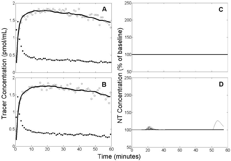
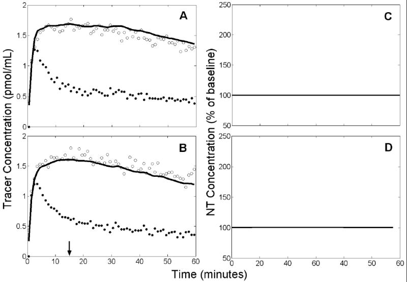
Analyses of null data via either method typically found little or no NT response. Figure 7 shows a representative ART fit to null data and the estimated NT profile family. The NT responses estimated from null data were characterized by small peak height (112±10% of baseline for ART; 107±13% of baseline for REF) and large temporal variance (σ(t̂_D)=10.78 min, σ(t̂_P)=9.69 min using ART; σ(t̂_D)=14.82 min, σ(t̂_P)=11.94 min using REF). Over 95% of the NT profile families estimated by ART from null data had an average peak height less than 129% of baseline. Thus, we designated 129% of baseline as the “95% confidence threshold” for families of NT curves estimated from PET data at this noise level (ζ = 0.03; see Eq 7). The 95% confidence threshold for the REF method based on these same data was 131%.

Figure 7.

Example of results obtained from simulated null data by applying ART using a noisy, unbiased TIF. Left panels (A,B): simulated PET data (open circles), measured plasma input (black circles), and model fit to the data (solid black curve). Right panels (C,D): estimated NT responses (black curves) from different initial parameter guesses. Top panels (A,C) refer to rest condition, bottom panels (B,D) to activation. There are 13 retained NT responses shown in D.

Data with NT Response

An ART example fit to PET data and the estimated NT profile family are shown in Figure 8. The average peak heights of the NT profile families estimated by both the ART and REF methods from simulated data with an authentic NT response typically exceeded the 95% confidence thresholds. All data sets analyzed by ART yielded NT response families with average peak heights exceeding the ART 95% confidence threshold. 149 of 150 NT profile families estimated by REF exceeded the REF 95% threshold. See Table 1 (lines 1-6) for a listing of false classification rates.

Figure 8.

Example of results obtained from data with true NT response by applying ART using a noisy, unbiased TIF. Left panels (A,B): simulated PET data (open circles), measured plasma input (black circles), and model fit to the data (solid black curve). Right panels (C,D): estimated NT responses (solid, thin curves) based on different initial parameters guesses and true NT curve (heavy, dashed curve). Top panels (A,C) apply to rest condition, bottom panels (B,D) to activation. There are 20 retained NT responses shown in D.

Figure 9 presents the performance of the ART and REF methods for NT events occurring at different times during the scan session. In the upper and middle panels of Figure 9, t̂_D and t̂_P estimated from 25 data sets containing the same true NT response for every delay time are plotted against their respective true values. F̂^NT (t̂_P) is plotted as a function of t_D in the bottom panel of Figure 9. For comparison, ΔBP measured from the curves is also provided. Figure 9 is based on unbiased TIFs only. For early NT release (t_D≤15 min), the ART method estimated delay time with slightly less bias than did REF; for later NT release, REF estimates of delay time were closer to the true values. ART and REF both overestimated peak time by several minutes, but ART generally showed slightly smaller bias. Peak height was consistently underestimated by both methods. Parameters estimated by ART tended to have slightly lower variance than those estimated by REF, particularly for early NT events.

Figure 9.

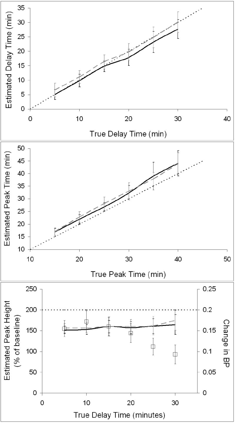
Values of key NT parameters (i.e., delay time, peak time, and peak height) estimated by ART and REF using unbiased TIFs. ART estimates are indicated by black curves and REF estimates by dashed gray curves. The line of identity is indicated by a think dotted black line. Top panel pertains to delay time, middle panel to peak time, and bottom panel to peak height. Measured changes in BP, indicated by square symbols, are included on peak height plot for comparison.

II.a. Biased TIFs: Effect on ART Method

Null Data

Average peak heights of NT profile families estimated by ART from null data with slow tracer metabolism were 118±14% of baseline and 155±26% of baseline for moderate metabolism. The false positive rate for slow metabolism was 22% but jumped to 90% for moderate metabolism. Variance in timing parameters estimated from null data with slow metabolism was large (σ(t̂_D)=16.17 min, σ(t̂_P)=15.36 min). Moderate metabolism gave less temporal uncertainty than slow metabolism (σ(t̂_D)=6.07 min, σ(t̂_P)=4.81 min). The model was unable to fit the data when rapid metabolism of the tracer was uncorrected.

Data with NT Response

Figure 10 displays overall performance of the ART method in the presence of uncorrected metabolism. Delay time was accurately estimated if metabolism was slow but overestimated if it was moderate. Peak time was consistently overestimated with large variance for slow metabolism, but correlation with the true values was high (R²=0.96). Moderate metabolism prevented any meaningful estimation of peak time. For both rates of metabolism, variance in estimated peak height was greatest for late responses. Peak height was consistently underestimated by ART using biased TIFs. See Table 1 (lines 8-13 and 15-20) for the associated false negative rates.

Figure 10.

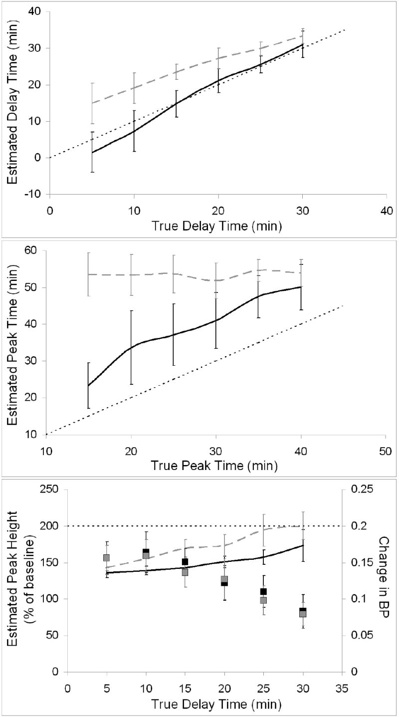
Key NT parameters estimated by ART using biased TIFs. Estimates from data with slow metabolism are indicated by black curves and estimates from data with moderate metabolism by dashed gray curves. The line of identity is indicated by a think dotted black line. Top panel pertains to delay time, middle panel to peak time, and bottom panel to peak height. Measured changes in BP (slow metabolism indicated by black squares, moderate metabolism by gray squares) are included on peak height plot for comparison.

II.b. Biased TIFs: Effect on REF Method

Null Data

The peak heights estimated by the REF method from null data with non-ideal reference regions were similar to those estimated using unbiased TIFs. The frequency of false positive events for RDR_R:T 1:5 and RDR_R:T 2:5 are reported in Table 1 (see lines 28 and 35). In no case was the false positive rate greater than 4%, nor did extent of receptor density in the reference region correlate with number of false positives. The estimated NT profiles were temporally incoherent; both σ(t_D) and σ(t_P) were greater than 10 minutes for all cases.

Data with NT Response

Figure 11 demonstrates the ability of the REF method to determine the NT profile if TIFs are biased. The two cases with greatest amounts of binding in the reference region, RDR_R:T 1:5 and RDR_R:T 2:5, are shown. Peak time is consistently overestimated but peak height estimates are not dependent on the timing of NT release. The rate of false negative findings was low and did not correlate with density of receptors in the reference region or with timing of NT response (see Table 1, lines 22-27 and 29-34). Variances of the estimated parameters were greater for later NT release, but generally similar to those observed using unbiased TIFs.

Figure 11.

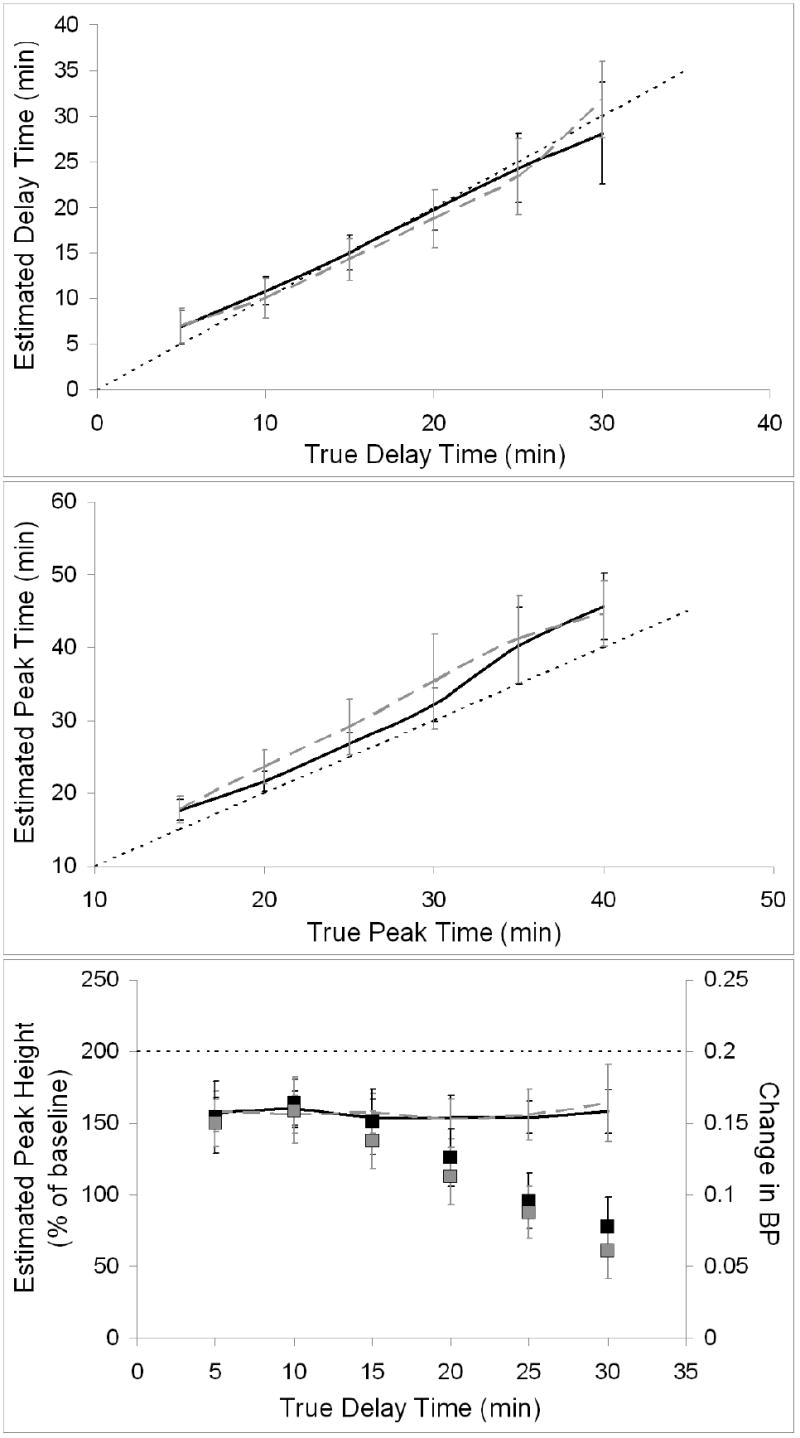
Estimated values of key NT parameters obtained by applying REF using biased TIFs. Results from the two cases with most heavily biased inputs (most binding in reference region) are shown. Black curves correspond to data with reference-to-target receptor density ratio (RDR_R:T) of 1:5 and dashed grey curves correspond to data with RDR_R:T of 2:5. The line of identity is indicated by a think dotted black line. Top panel pertains to delay time, middle panel to peak time, and bottom panel to peak height. Measured changes in BP (RDR_R:T 1:5 indicated by black squares, RDR_R:T 2:5 by grey squares) are included on peak height plot for comparison.

III. Altered Tracer Delivery

III.a. Changes in Blood Flow

Null Data

For all cases, estimated NT profiles had consistently small magnitude and large temporal uncertainty. Peak height estimated by REF was 111±13% of baseline when BF^REF decreased. For increased BF^TAR and decreased BF^REF, REF estimated a peak height of 109±12%. Analysis of these same data with ART (which used only the target region TACs) resulted in an estimated peak height of 112±8%. See Table 1 (lines 37 and 39) for the false positive frequencies associated with each of these cases. Standard deviation of timing parameters was greater than 11 min for all analyses of null data with activation-induced flow alterations.

Data with NT Response

The effects of altered blood flow on analysis of data with an authentic NT response were minor. Peak height estimated by REF was not affected by either decrease in BF^REF or BF^TAR increase with concurrent BF^REF decrease. Similarly, the peak height estimated by ART was not changed by increased BF^TAR. No false negative events were found for any of these cases (see lines 36 and 38 in Table 1).

III.b. Changes in Initial Tracer Uptake Constant

Null Data

The NT profiles estimated from null data with altered K₁ or ${\mathrm{K}}_1^{\mathrm{REF}}$ had very small peak height and large temporal variance. Figure 12 shows a representative REF fit and the family of estimated NT profiles from null data that were simulated with a decrease in ${\mathrm{K}}_1^{\mathrm{REF}}$ beginning at 15 min. Note that the model fit is poor (residuals are predominantly negative in the rest scan and positive in the activation scan) due to the incompatibility of the reference region TAC (and thus the TIF derived from it) in the activation condition with all other data. The NT curves estimated from null data sets containing decrease in ${\mathrm{K}}_1^{\mathrm{REF}}$ are characterized by very small magnitudes, with average peak height 100±1% of baseline. REF analysis of null data sets yielded an estimated peak height 100±0% of baseline if K₁ increased and ${\mathrm{K}}_1^{\mathrm{REF}}$ decreased. Peak height estimated by ART was 102±3% if initial uptake increased in the target region. No false positives were found in any of these cases (see Table 1, lines 41 and 43).

Figure 12.

Example of results obtained by applying REF to null data with a 10% decrease of ${\mathrm{K}}_1^{\mathrm{REF}}$ at 15 min. Left panels (A,B): simulated PET data (open circles), measured plasma input (black circles), and model fit to the data (solid black curve). Arrow indicates time at which ${\mathrm{K}}_1^{\mathrm{REF}}$ was decreased. Right panels (C,D): estimated NT responses (black curves) from different initial parameter guesses. Top panels (A,C) apply to rest condition, bottom panels (B,D) to activation. Note that the model fit is poor due to the incompatibility of the reference region TAC (and thus the TIF derived from it) in the activation condition with all other data. In addition to poor fits to the data, model insufficiency resulted in the failure of many initial guesses to converge. Thus, only 3 NT responses were retained (shown in D).

Data with NT Response

Simulated changes in K₁ and/or ${\mathrm{K}}_1^{\mathrm{REF}}$ alone exacerbated the underestimation of peak height from simulated data containing NT release. REF estimated the peak height to be 145±19% of baseline when ${\mathrm{K}}_1^{\mathrm{REF}}$ decreased. If K₁ increased, peak height estimated by ART was 143±17%. REF estimates of peak height decreased considerably if K₁ increased and ${\mathrm{K}}_1^{\mathrm{REF}}$ decreased. In this case, estimated peak height was 109±11%. False negative rates were large, particularly for K₁ increase with ${\mathrm{K}}_1^{\mathrm{REF}}$ decrease (refer to Table 1, lines 40 and 42).

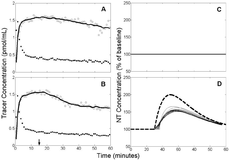
Alterations of K₁ and/or ${\mathrm{K}}_1^{\mathrm{REF}}$ alone exhibited varied effects on the accuracy of estimated NT timing parameters. Figure 13 shows a typical REF fit and the estimated NT profile family for the case of an NT response accompanied by a simultaneous decrease of ${\mathrm{K}}_1^{\mathrm{REF}}$. The estimated NT curves are temporally coherent and resemble a slightly delayed version of the true response. Decreased ${\mathrm{K}}_1^{\mathrm{REF}}$ increased the REF overestimation of delay time (bias(t̂_D)=3.31 min vs 1.33 min with no model violations). ART also overestimated delay time (bias(t̂_D)=2.44 min vs -0.21 min with no model violations) when K₁ increased. K₁ increase with concurrent ${\mathrm{K}}_1^{\mathrm{REF}}$ decrease caused REF to estimate both timing parameters inaccurately (bias(t̂_D)=−4.89 min, bias (t̂_P)=−4.60 min) and imprecisely (σ(t̂_D)=12.91 min, σ(t̂_P)=9.08 min).

Figure 13.

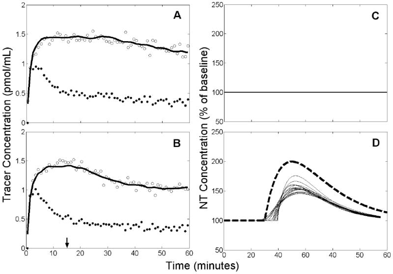
Example of results obtained by applying REF to data with a true NT response and 10% decrease of ${\mathrm{K}}_1^{\mathrm{REF}}$ at 15 min. Left panels (A,B): simulated PET data (open circles), measured plasma input (black circles), and model fit to the data (solid black curve). Arrow indicates time at which ${\mathrm{K}}_1^{\mathrm{REF}}$ decreased and NT response commenced. Right panels (C,D): estimated NT response (thin solid curves) and true NT curve (heavy dashed curve). Top panels (A,C) apply to rest condition, bottom panels (B,D) to activation. There are 18 retained NT responses shown in D.

III.c. Effects of Altered Tracer Delivery on Detection Ability

We looked at a number of possible scenarios that involved alteration of blood flow parameters. To summarize the detection ability of the ART and REF models in the face of changes in blood flow parameters, we present detection results via receiver operating characteristic (ROC) curves. ROC curves for analyses of data with changes in tracer delivery are shown in Figure 14. Circles on the figure indicate our chosen operating point, based upon the 95% confidence thresholds obtained from null data with constant flow parameters and unbiased TIFs. Figure 14A demonstrates that simulated changes in blood flow did not seriously compromise the detection ability of either the ART or the REF method. False positive rates remained consistent with those from data with constant flow parameters. Figure 14B shows the ability of each method to detect a true NT response if K₁ and/or ${\mathrm{K}}_1^{\mathrm{REF}}$ change during activation (but k₂ and ${\mathrm{k}}_2^{\mathrm{REF}}$ do not). Because the alterations in tracer delivery tended to decrease the height of the estimated NT profiles in the true activation and null cases, both the true positive and false positive rates were decreased. In fact, when K₁ increased and ${\mathrm{K}}_1^{\mathrm{REF}}$ decreased, 96% of true NT responses were below the 95% confidence threshold established for REF analysis.

Figure 14.

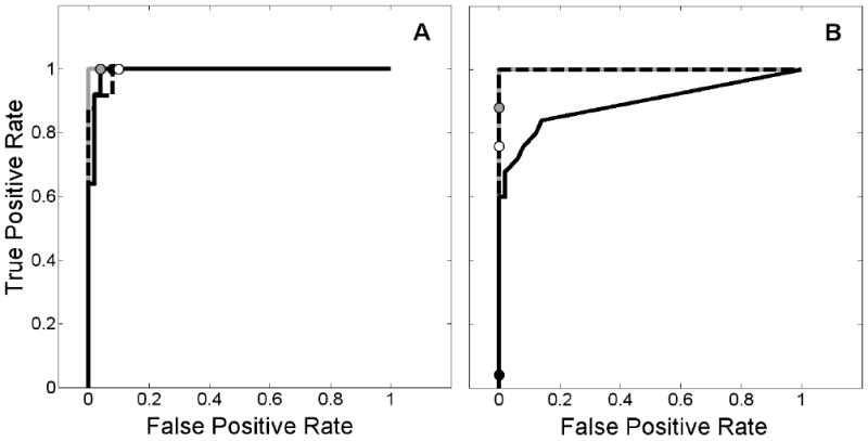
Receiver operating characteristic (ROC) curves demonstrating the effect of altered tracer delivery on the ability of ART and REF to detect neurotransmitter release events. 95% confidence thresholds are indicated by circles to show the chosen operating point. Left panel (A) corresponds to changes in blood flow, right panel (B) to changes in K₁ and/or ${\mathrm{K}}_1^{\mathrm{REF}}$. ROC curve for ART applied to data with increased delivery to target region is shown as solid gray curve (threshold: gray circle), REF applied to data with increased delivery to target region and decreased delivery to reference region displayed as solid black curve (threshold: solid black circle), and REF applied to data with decreased delivery to reference region only plotted as dashed black curve (threshold: white circle). In B, solid gray and dashed black curves overlay one another.

DISCUSSION

The present work examines the temporal precision of two variants of ntPET and assesses the performance of the methods when confronted with likely violations of model assumptions. In addition, we compare the ART and REF formulations and determine under what conditions the use of a reference region-derived TIF is an acceptable alternative to arterial blood sampling. We develop these ideas here, explore some technical details of the methods, and consider the complementary roles that ntPET and microdialysis could play in studying neurotransmission in vivo.

A. Temporal Precision of ntPET

The temporal precision of ntPET varies slightly with the timing of the NT response. In general, performance is better when NT release occurs early rather than late in the scan. Absent model violations, the precision of estimated delay time, t̂_D, is approximately σ(t̂_D)=2 min using ART and σ(t̂_D)=2.5 min using REF for early NT events (defined as true t_P=15 to 25 min); uncertainty of estimated peak time, t̂_p, is less than 2 min with ART and 2-2.5 min with REF. The error in estimated timing parameters tends to increase as the NT response occurs later in time. With the ART method we find σ(t̂_D)<4 min and σ(t̂_P)≈4.5 min when data have late NT responses (defined as true t_P=30 to 40min). Under similar conditions, the REF method estimates both timing parameters with comparable variance (σ(t̂_D)≈σ(t̂_P)≈3.5 min). We have shown previously that the precision of estimated parameters improves with the prominence of the NT profile (i.e., larger magnitude and greater sharpness of the NT response, and higher PET signal-to-noise ratio) (Normandin and Morris, 2006).

The ability of ntPET to characterize NT dynamics represents a potential advance in PET analysis. The temporal resolution that we report here may be sufficient to provide answers that have previously eluded researchers. For instance, PET investigators have compared the kinetics of cocaine and methylphenidate (Volkow et al., 1995; Volkow et al., 1999) and the effects of long- and short-acting methylphenidate (Spencer et al., 2006), and surmised that the speed of their respective dopamine responses may predict their addictive liabilities. However, it would be impossible to test this hypothesis with PET by measuring change in binding potential. In recent work investigating conditioned NT release, Boileau et al. (2007) found that the change in raclopride binding potential after amphetamine was the same as after placebo, but the behavioral effects persisted longer after drug. They speculated that amphetamine- and placebo-induced dopamine responses may have distinct temporal characteristics, but lamented the inability of PET to resolve such a difference. We believe that, coupled with an appropriate analysis technique, PET could discern different temporal profiles in NT responses. Answers to questions about the time course of NT release may be attainable through ntPET analysis.

B. Performance of ntPET Under Conditions of Model Violations

We examined plausible violations of model assumptions and evaluated their respective impacts on the results of ntPET. Many violations failed to undermine the method. The violations that did degrade model performance were either correctable (presence of labeled metabolites in the blood) or physiologically ambiguous (instantaneous changes in K₁ and/or ${\mathrm{K}}_1^{\mathrm{REF}}$ without accompanying changes in k₂ or ${\mathrm{k}}_2^{\mathrm{REF}}$).

Uncorrected Metabolites in Blood

The uncorrected presence of labeled metabolites in the plasma is a likely corruption of the measured TIFs used by ART. TACs decrease more quickly than they would otherwise, which could be attributed to faster tracer efflux or a sustained release of NT. This corruption of the input data causes a progressive bias with time and degrades the performance of ART. Therefore, when using the ART method, we recommend that metabolite correction be performed unless tracer metabolism is known to be very limited. Population-based corrections may not be adequate because rates of tracer metabolism can be highly variable between subjects (Gillings et al., 2001; Ishiwata et al., 1998) and can be influenced by drug treatments (Cumming et al., 1999). We speculate that the complexity of the ntPET models, in particular the desired endpoint (a full characterization of the NT response), makes the method more sensitive to biases in the TIF than conventional PET models. The previously demonstrated sensitivity of multiple tracer injection experiments to errors in the calculated input functions (Morris et al., 1999) supports this conjecture.

Specific Binding in Reference Region

Reference region-derived TIFs could be biased by specific binding in the reference region, a common problem for non-dopaminergic NT systems (Litton et al., 1994; Logan et al., 2005) or for dopaminergic imaging with high affinity tracers (Asselin et al., 2007; Christian et al., 2004; Delforge et al., 1999; Pinborg et al., 2007). The presence of receptors in the reference region increases tracer retention and, coupled with the errant assumption of no receptors, lends the appearance of lower than expected initial uptake in the target region than the reference region. This violation manifests itself as an underestimation of R₁ (=K₁/ ${\mathrm{K}}_1^{\mathrm{REF}}$). Fortunately, the use of imperfect reference regions neither biases the temporal accuracy nor degrades the temporal precision of the REF method. Different amounts of specific binding in the reference region yield TIFs of different magnitudes but similar shape throughout most of the scan (see Figure 4). In the present simulations of raclopride TACs, the derived TIF is dominated by the plateau that follows the early peak. Consistency in the shape of the resultant TIFs probably explains the insensitivity of REF to binding in the reference region.

Flow Parameters Altered by Activation

Activation-induced changes in blood flow are likely to be encountered following many NT-releasing tasks. Such changes have been observed after ethanol administration using H₂[¹⁵O] PET (Volkow et al., 1988). Our demonstration that alterations to the shapes of TACs caused by simulated changes in blood flow are negligible is in agreement with previous work (Alpert et al., 2003; Pappata et al., 2002), and any changes in the curves are well below the level of noise in typical data. Thus, changes in blood flow should not appreciably impact ntPET results.

If it were physiologically possible, alteration of K₁ and/or ${\mathrm{K}}_1^{\mathrm{REF}}$ alone could influence results obtained with ntPET. The trajectory of the target region TAC rises when K₁ is increased (see Figure 5B). Release of NT has the opposite effect because it displaces the tracer from binding sites and lowers the TAC. When these two effects occur simultaneously they counteract one another, and the peak height of the NT response estimated by ART is attenuated. Similarly, a decrease of ${\mathrm{K}}_1^{\mathrm{REF}}$ reduces the magnitude of the NT responses estimated by REF. In these two cases, the sensitivity of ntPET is reduced but useful results may still be obtained. However, if K₁ is increased and ${\mathrm{K}}_1^{\mathrm{REF}}$ decreased, the NT responses estimated by REF will be completely nullified. To achieve greater sensitivity, one might consider lowering the threshold value. Unfortunately, even setting the threshold as low as 103% of baseline would yield a true positive detection rate of only 0.72. In addition, such a low threshold would lead to an unacceptably large false positive rate (0.46) if the expected model violations did not occur. Thus, a modification of the threshold is not a viable correction to ntPET for the case of K₁ increase coupled with ${\mathrm{K}}_1^{\mathrm{REF}}$ decrease.

The physiological likelihood of isolated changes in K₁ remains unresolved (Alpert et al., 2003; Logan et al., 1994; Pappata et al., 2002). Nevertheless, our simulated tests with K₁ alterations represent worst case scenarios. Change in flow parameters may not coincide with NT release (Schwarz et al., 2004), and would probably depend upon the type of stimulus and might vary between individuals. With regard to our specific interest in alcohol-induced dopamine release, the simulated changes in K₁ and ${\mathrm{K}}_1^{\mathrm{REF}}$, which were chosen to simulate the alcohol-induced blood flow alterations reported by Volkow et al. (1988), should not cause false positive findings; rather, false negatives would result (refer to Figure 14 and lines 40 and 42 of Table 1). Thus, any supra-threshold NT profiles estimated from data in subjects receiving alcohol could be confidently attributed to NT release. In practice, the threshold value may be established based on evaluations of rest-rest studies (the experimental null case) and/or simulations that appropriately represent the acquired data.

C. Comparison of ART and REF

The ART formulation of ntPET performs slightly better than REF, provided that (1) NT responses occur early in the scan, (2) unbiased TIFs are available, and (3) the PET data are free of activation-induced changes in tracer delivery. Figure 15 summarizes the respective performance of the methods by plotting the average estimated peak height against the average estimated peak time for ART and REF analyses of each data set that does not contain model violations. The points cluster more tightly for ART (shown at left) than REF, particularly for early NT events (darker markers). The performance advantage of ART over REF is less evident if NT responses occur later in the scan.

Figure 15.

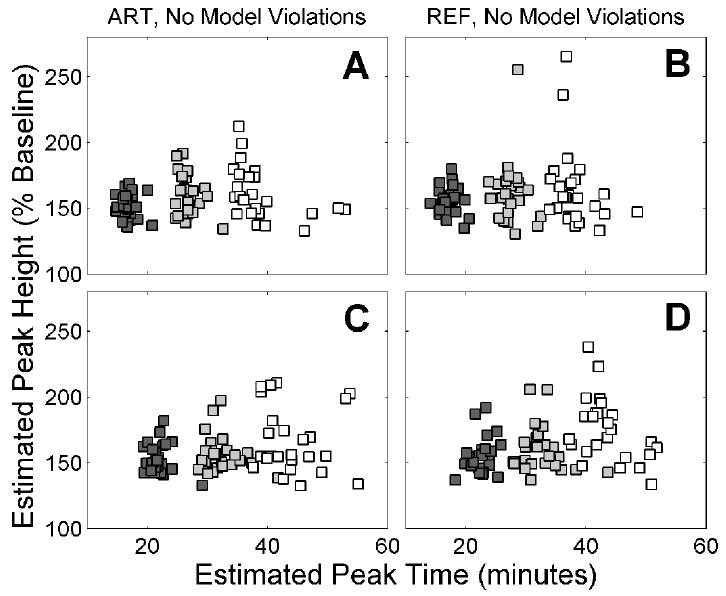
Estimated peak height of NT response, [F̂^NT (t̂_P)/Basal]×100%, plotted against estimated peak time, t̂_P. ART results are shown on left panels, REF on right panels. Data sets with NT responses separated by 10 min are shown on the upper (A,B) and lower (C,D) panels, with different colored markers indicating different NT timing. A,B: true t_P=15 min for dark grey, t_P=25 min for light grey, t_P=35 min for white. C,D: A,B: true t_P=20 min for dark grey, t_P=30 min for light grey, t_P=40 min for white.

The two variants of ntPET behaved very differently when presented with realistically biased TIFs: ART performance deteriorated even with slow tracer metabolism, but REF was insensitive to specific binding in the reference region. Neither method was appreciably impaired by an activation stimulus that also caused a change in blood flow. A strength of the ART method is that it requires PET data from the target region only, whereas REF needs data from the target and a reference region. Thus, biases in either region could theoretically cause artifacts in REF analyses. If biases are present in both regions and in opposite directions (e.g., K₁ increases and ${\mathrm{K}}_1^{\mathrm{REF}}$ decreases) the impact on REF is severe. On the other hand, should the biases occur in the same direction (e.g., a “global” change in K₁), the REF method performs better than ART because the kinetic artifacts in the two regions counteract one another (data not shown). In other words, a global change in K₁ leads to a reference region-derived TIF that is consistent with the target region TAC, whereas the plasma curve is not. Unless the investigator specifically expects that the particular stimulus will increase K₁ and decrease ${\mathrm{K}}_1^{\mathrm{REF}}$ (or vice versa), we recommend the REF variant of ntPET as an alternative to ART that is more convenient, nearly as precise, and more robust to plausible corruptions of the TIF.

D. Technical Details

Peak Time Constraint

Use of the peak time constraint marks an improvement over our original implementation of ntPET (Morris et al., 2005). This penalty term increases the value of the cost function if the peak of the NT response occurs outside the scan window. The peak time constraint has little effect if NT release peaks during PET acquisition, but it has a useful impact if there is no NT response (i.e., null data). If the peak time constraint were not used, the fitting routine would be free to find NT responses that peak before or after the scan. Since there are no data at these times to dictate the amplitude of the response, the estimated NT profiles could have very large magnitude. The net effect, if we included peaks outside the scan window, would be to force a higher 95% confidence threshold (based on null data), and thus accept more false negative events from data with bona fide NT responses.

Characteristics of Estimated Peak Height

Peak height is consistently underestimated, as demonstrated by Figure 8 and lower panels of Figures 9-11. Absolute scale is not identifiable, but fractional scale (relative to basal NT level) can be determined. Peak height estimates have greater variability than do the timing parameters, particularly for early NT responses (see Figure 15). Previous work (Normandin and Morris, 2006) has shown that underestimation of peak height is also observed with larger NT responses, but that the estimated peak height correlates with the true value. Although peak height is underestimated, the bias tends to be fairly consistent across a wide range of NT response times (see bottom panel of Figures 9-11). This consistency contrasts with estimates of ΔBP, which have been shown to be conflated with NT timing (Morris and Yoder, 2007; Yoder et al., 2004: see also bottom panels of Figures 9-11). Because F̂^NT (t̂_P) does not vary with NT response time, the peak height estimated by ntPET may be a more consistent measure of the magnitude of NT release than the commonly used ΔBP.

Parameter Estimation, Restrictions, and Identifiability

Parameter estimation was performed using the MATLAB function ‘lsqcurvefit’, a Levenberg-Marquardt algorithm. Convergence tolerances for function and parameter values (‘TolFun’ and ‘TolX’, respectively, in MATLAB optimization settings) were both set to 10^-9. A given fit was terminated and considered non-converging if the number of iterations reached 400.

In the present studies, we have fixed B_max, ${\mathrm{k}}_{\mathrm{on}}^{\mathrm{NT}}$, and ${\mathrm{k}}_{\mathrm{off}}^{\mathrm{NT}}$ (Fisher et al., 1995; Morris et al., 1995), and restricted γ to nonnegative values in order to detect only increases in NT. Future work to improve the practicality of the method will include efforts to reduce computational load and sensitivity to initial guess by fixing more parameters. This may be possible given sufficient preliminary data for a given tracer (i.e., prior knowledge of Θ_TR).

We acknowledge that identifiability of parameters is a potential problem. We have sought to address this concern by using a constrained optimization routine that aids identifiability and by fitting the data with many different, randomly selected initial guesses. Our results with multiple initial guesses demonstrate that while a unique, global minimum in parameter space may not be attainable, the recovered neurotransmitter responses are generally consistent for a given data set. Note that this consistency is in stark contrast to the neurotransmitter profiles associated with the initial parameter guesses, examples of which are shown in Figure 6. It should also be emphasized that the neurotransmitter timing parameters are largely insensitive to the choice of tracer parameters. Finally, we reiterate that the goal of ntPET analysis is the determination of the neurotransmitter profile – that is, for our purposes the tracer parameters can be considered “nuisance” parameters.

E. ntPET as a Complement to Microdialysis

ntPET shares a common goal with microdialysis, namely, characterization of the time course of neurotransmitter concentration. Microdialysis is used extensively in neurochemical studies on animals, but requires placement of probes into the brain for direct assay of chemical species. Though ntPET and microdialysis are similar in their objective, their respective endpoints are dissimilar. For example, amphetamine and methylphenidate have been shown to cause comparable changes in intrasynaptic dopamine (as determined by ΔBP from PET) but different effects on extracellular dopamine (measured by microdialysis) (Schiffer et al., 2006b). Microdialysis samples from the extracellular fluid, whereas the PET signal and a proper model measure the effects of intrasynaptic binding and displacement of tracer. ntPET cannot be readily performed on awake rodents or provide sequential measurements over several days as can be done with microdialysis. On the other hand, ntPET is non-invasive and can be performed on humans. The collateral effects of microdialysis on brain physiology have recently been questioned, particularly with regard to probe-induced damage to tissue integrity (Bungay et al., 2003; Tang et al., 2003), cerebral metabolism (Frumberg et al., 2007; Schiffer et al., 2006a), and animal behavior (Frumberg et al., 2007). These alterations will not be caused by ntPET. Nevertheless, ntPET and microdialysis may represent complementary techniques to resolve difference between intra- and extra-synaptic neurotransmitter fluctuations. If the relationship between microdialysis and ntPET can be determined, the vast microdialysis literature could be mined to suggest a large number of informative, translational studies in human subjects.

CONCLUSIONS

This simulation study evaluated two alternative formulations of ntPET under idealized conditions (noisy but unbiased data) and when confronted with plausible model violations. The ART formulation of ntPET, which obtains the tracer input function from arterial blood samples, was sensitive to the presence of labeled metabolites in the plasma that were left uncorrected. The REF variant of ntPET, which derives the tracer input function from reference region PET data, was robust to specific binding in the reference region. Neither ART nor REF was significantly influenced by changes in blood flow. However, the performance of both methods was impaired by changes in K₁ decoupled from changes in k₂. The accuracy of conventional ΔBP measurements was also degraded by changes in K₁ alone. ΔBP is known to be compromised by the timing of NT release, whereas ntPET proved to be robust. Under most circumstances, the REF formulation of ntPET is an appropriate alternative to the more demanding ART method.

References

- Alpert NM, Badgaiyan RD, Livni E, Fischman AJ. A novel method for noninvasive detection of neuromodulatory changes in specific neurotransmitter systems. Neuroimage. 2003;19:1049–1060. doi: 10.1016/s1053-8119(03)00186-1. [DOI] [PubMed] [Google Scholar]
- Asselin MC, Montgomery AJ, Grasby PM, Hume SP. Quantification of PET studies with the very high-affinity dopamine D2/D3 receptor ligand [11C]FLB 457: re-evaluation of the validity of using a cerebellar reference region. J Cereb Blood Flow Metab. 2007;27:378–392. doi: 10.1038/sj.jcbfm.9600340. [DOI] [PubMed] [Google Scholar]
- Aston JA, Gunn RN, Worsley KJ, Ma Y, Evans AC, Dagher A. A statistical method for the analysis of positron emission tomography neuroreceptor ligand data. Neuroimage. 2000;12:245–256. doi: 10.1006/nimg.2000.0620. [DOI] [PubMed] [Google Scholar]
- Bertoldo A, Sparacino G, Cobelli C. “Population” approach improves parameter estimation of kinetic models from dynamic PET data. Medical Imaging, IEEE Transactions on. 2004;23:297–306. doi: 10.1109/TMI.2004.824243. [DOI] [PubMed] [Google Scholar]
- Blomqvist G, Pauli S, Farde L, Eriksson L, Persson A, Halldin C. Maps of receptor binding parameters in the human brain--a kinetic analysis of PET measurements. Eur J Nucl Med. 1990;16:257–265. doi: 10.1007/BF00842777. [DOI] [PubMed] [Google Scholar]
- Boileau I, Dagher A, Leyton M, Welfeld K, Booij L, Diksic M, Benkelfat C. Conditioned dopamine release in humans: a positron emission tomography [11C]raclopride study with amphetamine. J Neurosci. 2007;27:3998–4003. doi: 10.1523/JNEUROSCI.4370-06.2007. [DOI] [PMC free article] [PubMed] [Google Scholar]
- Buchsbaum MS, Christian BT, Lehrer DS, Narayanan TK, Shi B, Mantil J, Kemether E, Oakes TR, Mukherjee J. D2/D3 dopamine receptor binding with [F-18]fallypride in thalamus and cortex of patients with schizophrenia. Schizophr Res. 2006;85:232–244. doi: 10.1016/j.schres.2006.03.042. [DOI] [PubMed] [Google Scholar]
- Bungay PM, Newton-Vinson P, Isele W, Garris PA, Justice JB. Microdialysis of dopamine interpreted with quantitative model incorporating probe implantation trauma. J Neurochem. 2003;86:932–946. doi: 10.1046/j.1471-4159.2003.01904.x. [DOI] [PMC free article] [PubMed] [Google Scholar]
- Christian BT, Narayanan T, Shi B, Morris ED, Mantil J, Mukherjee J. Measuring the in vivo binding parameters of [18F]-fallypride in monkeys using a PET multiple-injection protocol. J Cereb Blood Flow Metab. 2004;24:309–322. doi: 10.1097/01.WCB.0000105020.93708.DD. [DOI] [PubMed] [Google Scholar]
- Cumming P, Yokoi F, Chen A, Deep P, Dagher A, Reutens D, Kapczinski F, Wong DF, Gjedde A. Pharmacokinetics of radiotracers in human plasma during positron emission tomography. Synapse. 1999;34:124–134. doi: 10.1002/(SICI)1098-2396(199911)34:2<124::AID-SYN5>3.0.CO;2-O. [DOI] [PubMed] [Google Scholar]
- Cunningham VJ, Hume SP, Price GR, Ahier RG, Cremer JE, Jones AK. Compartmental analysis of diprenorphine binding to opiate receptors in the rat in vivo and its comparison with equilibrium data in vitro. J Cereb Blood Flow Metab. 1991;11:1–9. doi: 10.1038/jcbfm.1991.1. [DOI] [PubMed] [Google Scholar]
- Delforge J, Bottlaender M, Loc’h C, Guenther I, Fuseau C, Bendriem B, Syrota A, Maziere B. Quantitation of extrastriatal D2 receptors using a very high-affinity ligand (FLB 457) and the multi-injection approach. J Cereb Blood Flow Metab. 1999;19:533–546. doi: 10.1097/00004647-199905000-00008. [DOI] [PubMed] [Google Scholar]
- Delforge J, Syrota A, Mazoyer BM. Experimental design optimisation: theory and application to estimation of receptor model parameters using dynamic positron emission tomography. Phys Med Biol. 1989;34:419–435. doi: 10.1088/0031-9155/34/4/002. [DOI] [PubMed] [Google Scholar]
- Delforge J, Syrota A, Mazoyer BM. Identifiability analysis and parameter identification of an in vivo ligand-receptor model from PET data. IEEE Trans Biomed Eng. 1990;37:653–661. doi: 10.1109/10.55673. [DOI] [PubMed] [Google Scholar]
- Dewey SL, Smith GS, Logan J, Brodie JD, Simkowitz P, MacGregor RR, Fowler JS, Volkow ND, Wolf AP. Effects of central cholinergic blockade on striatal dopamine release measured with positron emission tomography in normal human subjects. Proc Natl Acad Sci U S A. 1993;90:11816–11820. doi: 10.1073/pnas.90.24.11816. [DOI] [PMC free article] [PubMed] [Google Scholar]
- Endres CJ, Kolachana BS, Saunders RC, Su T, Weinberger D, Breier A, Eckelman WC, Carson RE. Kinetic modeling of [11C]raclopride: combined PET-microdialysis studies. J Cereb Blood Flow Metab. 1997;17:932–942. doi: 10.1097/00004647-199709000-00002. [DOI] [PubMed] [Google Scholar]
- Fedi M, Berkovic SF, Marini C, Mulligan R, Tochon-Danguy H, Reutens DC. A GABAA receptor mutation causing generalized epilepsy reduces benzodiazepine receptor binding. Neuroimage. 2006;32:995–1000. doi: 10.1016/j.neuroimage.2006.05.059. [DOI] [PubMed] [Google Scholar]
- Feng D, Huang SC, Wang X. Models for computer simulation studies of input functions for tracer kinetic modeling with positron emission tomography. Int J Biomed Comput. 1993;32:95–110. doi: 10.1016/0020-7101(93)90049-c. [DOI] [PubMed] [Google Scholar]
- Fisher RE, Morris ED, Alpert NM, Fischman AJ. In vivo imaging of neuromodulatory synaptic transmission using PET: A review of relevant neurophysiology. Human Brain Mapping. 1995;3:24–34. [Google Scholar]
- Friston KJ, Malizia AL, Wilson S, Cunningham VJ, Jones T, Nutt DJ. Analysis of dynamic radioligand displacement or “activation” studies. J Cereb Blood Flow Metab. 1997;17:80–93. doi: 10.1097/00004647-199701000-00011. [DOI] [PubMed] [Google Scholar]
- Frumberg DB, Fernando MS, Lee DE, Biegon A, Schiffer WK. Metabolic and behavioral deficits following a routine surgical procedure in rats. Brain Res. 2007 doi: 10.1016/j.brainres.2007.01.134. [DOI] [PMC free article] [PubMed] [Google Scholar]
- Gillings NM, Bender D, Falborg L, Marthi K, Munk OL, Cumming P. Kinetics of the metabolism of four PET radioligands in living minipigs. Nucl Med Biol. 2001;28:97–104. doi: 10.1016/s0969-8051(00)00187-6. [DOI] [PubMed] [Google Scholar]
- Heinz A, Ragan P, Jones DW, Hommer D, Williams W, Knable MB, Gorey JG, Doty L, Geyer C, Lee KS, Coppola R, Weinberger DR, Linnoila M. Reduced central serotonin transporters in alcoholism. Am J Psychiatry. 1998;155:1544–1549. doi: 10.1176/ajp.155.11.1544. [DOI] [PubMed] [Google Scholar]
- Huang SC, Bahn MM, Barrio JR, Hoffman JM, Satyamurthy N, Hawkins RA, Mazziotta JC, Phelps ME. A double-injection technique for in vivo measurement of dopamine D2-receptor density in monkeys with 3-(2’-[18F]fluoroethyl)spiperone and dynamic positron emission tomography. J Cereb Blood Flow Metab. 1989;9:850–858. doi: 10.1038/jcbfm.1989.119. [DOI] [PubMed] [Google Scholar]
- Innis RB, Cunningham VJ, Delforge J, Fujita M, Gjedde A, Gunn RN, Holden J, Houle S, Huang SC, Ichise M, Iida H, Ito H, Kimura Y, Koeppe RA, Knudsen GM, Knuuti J, Lammertsma AA, Laruelle M, Logan J, Maguire RP, Mintun MA, Morris ED, Parsey R, Price JC, Slifstein M, Sossi V, Suhara T, Votaw JR, Wong DF, Carson RE. Consensus nomenclature for in vivo imaging of reversibly binding radioligands. J Cereb Blood Flow Metab. 2007;27:1533–1539. doi: 10.1038/sj.jcbfm.9600493. [DOI] [PubMed] [Google Scholar]
- Innis RB, Malison RT, al-Tikriti M, Hoffer PB, Sybirska EH, Seibyl JP, Zoghbi SS, Baldwin RM, Laruelle M, Smith EO, et al. Amphetamine-stimulated dopamine release competes in vivo for [123I]IBZM binding to the D2 receptor in nonhuman primates. Synapse. 1992;10:177–184. doi: 10.1002/syn.890100302. [DOI] [PubMed] [Google Scholar]
- Ishiwata K, Itou T, Ohyama M, Yamada T, Mishina M, Ishii K, Nariai T, Sasaki T, Oda K, Toyama H, Senda M. Metabolite analysis of [11C]flumazenil in human plasma: assessment as the standardized value for quantitative PET studies. Ann Nucl Med. 1998;12:55–59. doi: 10.1007/BF03165418. [DOI] [PubMed] [Google Scholar]
- Koepp MJ, Gunn RN, Lawrence AD, Cunningham VJ, Dagher A, Jones T, Brooks DJ, Bench CJ, Grasby PM. Evidence for striatal dopamine release during a video game. Nature. 1998;393:266–268. doi: 10.1038/30498. [DOI] [PubMed] [Google Scholar]
- Kwong KK, Hopkins AL, Belliveau JW, Chesler DA, Porkka LM, McKinstry RC, Finelli DA, Hunter GJ, Moore JB, Barr RG, et al. Proton NMR imaging of cerebral blood flow using H2(17)O. Magn Reson Med. 1991;22:154–158. doi: 10.1002/mrm.1910220116. [DOI] [PubMed] [Google Scholar]
- Landaw EM, DiStefano JJ., 3rd Multiexponential, multicompartmental, and noncompartmental modeling. II. Data analysis and statistical considerations. Am J Physiol. 1984;246:R665–677. doi: 10.1152/ajpregu.1984.246.5.R665. [DOI] [PubMed] [Google Scholar]
- Laruelle M, Abi-Dargham A, van Dyck CH, Rosenblatt W, Zea-Ponce Y, Zoghbi SS, Baldwin RM, Charney DS, Hoffer PB, Kung HF, et al. SPECT imaging of striatal dopamine release after amphetamine challenge. J Nucl Med. 1995;36:1182–1190. [PubMed] [Google Scholar]
- Litton JE, Hall H, Pauli S. Saturation analysis in PET--analysis of errors due to imperfect reference regions. J Cereb Blood Flow Metab. 1994;14:358–361. doi: 10.1038/jcbfm.1994.45. [DOI] [PubMed] [Google Scholar]
- Logan J, Ding YS, Lin KS, Pareto D, Fowler J, Biegon A. Modeling and analysis of PET studies with norepinephrine transporter ligands: the search for a reference region. Nucl Med Biol. 2005;32:531–542. doi: 10.1016/j.nucmedbio.2005.04.005. [DOI] [PubMed] [Google Scholar]
- Logan J, Fowler JS, Volkow ND, Wang GJ, Ding YS, Alexoff DL. Distribution volume ratios without blood sampling from graphical analysis of PET data. J Cereb Blood Flow Metab. 1996;16:834–840. doi: 10.1097/00004647-199609000-00008. [DOI] [PubMed] [Google Scholar]
- Logan J, Fowler JS, Volkow ND, Wolf AP, Dewey SL, Schlyer DJ, MacGregor RR, Hitzemann R, Bendriem B, Gatley SJ, et al. Graphical analysis of reversible radioligand binding from time-activity measurements applied to [N-11C-methyl]-(-)-cocaine PET studies in human subjects. J Cereb Blood Flow Metab. 1990;10:740–747. doi: 10.1038/jcbfm.1990.127. [DOI] [PubMed] [Google Scholar]
- Logan J, Volkow ND, Fowler JS, Wang GJ, Dewey SL, MacGregor R, Schlyer D, Gatley SJ, Pappas N, King P, et al. Effects of blood flow on [11C]raclopride binding in the brain: model simulations and kinetic analysis of PET data. J Cereb Blood Flow Metab. 1994;14:995–1010. doi: 10.1038/jcbfm.1994.132. [DOI] [PubMed] [Google Scholar]
- Mach RH, Nader MA, Ehrenkaufer RL, Line SW, Smith CR, Gage HD, Morton TE. Use of positron emission tomography to study the dynamics of psychostimulant-induced dopamine release. Pharmacol Biochem Behav. 1997;57:477–486. doi: 10.1016/s0091-3057(96)00449-2. [DOI] [PubMed] [Google Scholar]
- Millet P, Ibanez V, Delforge J, Pappata S, Guimon J. Wavelet analysis of dynamic PET data: application to the parametric imaging of benzodiazepine receptor concentration. Neuroimage. 2000;11:458–472. doi: 10.1006/nimg.2000.0563. [DOI] [PubMed] [Google Scholar]
- Mintun MA, Raichle ME, Kilbourn MR, Wooten GF, Welch MJ. A quantitative model for the in vivo assessment of drug binding sites with positron emission tomography. Ann Neurol. 1984;15:217–227. doi: 10.1002/ana.410150302. [DOI] [PubMed] [Google Scholar]
- Morris ED, Alpert NM, Fischman AJ. Comparison of two compartmental models for describing receptor ligand kinetics and receptor availability in multiple injection PET studies. J Cereb Blood Flow Metab. 1996a;16:841–853. doi: 10.1097/00004647-199609000-00009. [DOI] [PubMed] [Google Scholar]
- Morris ED, Babich JW, Alpert NM, Bonab AA, Livni E, Weise S, Hsu H, Christian BT, Madras BK, Fischman AJ. Quantification of dopamine transporter density in monkeys by dynamic PET imaging of multiple injections of 11C-CFT. Synapse. 1996b;24:262–272. doi: 10.1002/(SICI)1098-2396(199611)24:3<262::AID-SYN9>3.0.CO;2-C. [DOI] [PubMed] [Google Scholar]
- Morris ED, Bonab AA, Alpert NM, Fischman AJ, Madras BK, Christian BT. Concentration of dopamine transporters: to Bmax or not to Bmax? Synapse. 1999;32:136–140. doi: 10.1002/(SICI)1098-2396(199905)32:2<136::AID-SYN7>3.0.CO;2-G. [DOI] [PubMed] [Google Scholar]
- Morris ED, Fisher RE, Alpert NM, Rauch SL, Fischman AJ. In vivo imaging of neuromodulation using positron emission tomography: Optimal ligand characteristics and task length for detection of activation. Human Brain Mapping. 1995;3:35–55. [Google Scholar]
- Morris ED, Yoder KK. Positron emission tomography displacement sensitivity: predicting binding potential change for positron emission tomography tracers based on their kinetic characteristics. J Cereb Blood Flow Metab. 2007;27:606–617. doi: 10.1038/sj.jcbfm.9600359. [DOI] [PubMed] [Google Scholar]
- Morris ED, Yoder KK, Wang C, Normandin MD, Zheng QH, Mock B, Muzic RF, Jr, Froehlich JC. ntPET: a new application of PET imaging for characterizing the kinetics of endogenous neurotransmitter release. Mol Imaging. 2005;4:473–489. doi: 10.2310/7290.2005.05130. [DOI] [PubMed] [Google Scholar]
- Muzic RF, Jr, Christian BT. Evaluation of objective functions for estimation of kinetic parameters. Med Phys. 2006;33:342–353. doi: 10.1118/1.2135907. [DOI] [PubMed] [Google Scholar]
- Muzic RF, Jr, Cornelius S. COMKAT: compartment model kinetic analysis tool. J Nucl Med. 2001;42:636–645. [PubMed] [Google Scholar]
- Muzic RF, Jr, Nelson AD, Saidel GM, Miraldi F. Optimal experiment design for PET quantification of receptor concentration. Medical Imaging, IEEE Transactions on. 1996;15:2–12. doi: 10.1109/42.481436. [DOI] [PubMed] [Google Scholar]
- Normandin MD, Morris ED. Temporal Resolution of ntPET Using Either Arterial or Reference Region-Derived Plasma Input Functions. Engineering in Medicine and Biology Society, 2006; EMBS ’06 28th Annual International Conference of the IEEE; 2006. pp. 2005–2008. [DOI] [PubMed] [Google Scholar]
- O’Sullivan F, Saha A. Use of ridge regression for improved estimation of kinetic constants from PET data. IEEE Trans Med Imaging. 1999;18:115–125. doi: 10.1109/42.759111. [DOI] [PubMed] [Google Scholar]
- Ogawa S, Lee TM, Kay AR, Tank DW. Brain magnetic resonance imaging with contrast dependent on blood oxygenation. Proc Natl Acad Sci U S A. 1990;87:9868–9872. doi: 10.1073/pnas.87.24.9868. [DOI] [PMC free article] [PubMed] [Google Scholar]
- Pappata S, Dehaene S, Poline JB, Gregoire MC, Jobert A, Delforge J, Frouin V, Bottlaender M, Dolle F, Di Giamberardino L, Syrota A. In vivo detection of striatal dopamine release during reward: a PET study with [(11)C]raclopride and a single dynamic scan approach. Neuroimage. 2002;16:1015–1027. doi: 10.1006/nimg.2002.1121. [DOI] [PubMed] [Google Scholar]
- Picard F, Bruel D, Servent D, Saba W, Fruchart-Gaillard C, Schollhorn-Peyronneau MA, Roumenov D, Brodtkorb E, Zuberi S, Gambardella A, Steinborn B, Hufnagel A, Valette H, Bottlaender M. Alteration of the in vivo nicotinic receptor density in ADNFLE patients: a PET study. Brain. 2006;129:2047–2060. doi: 10.1093/brain/awl156. [DOI] [PubMed] [Google Scholar]
- Pinborg LH, Videbaek C, Ziebell M, Mackeprang T, Friberg L, Rasmussen H, Knudsen GM, Glenthoj BY. [(123)I]Epidepride binding to cerebellar dopamine D(2)/D(3) receptors is displaceable: Implications for the use of cerebellum as a reference region. Neuroimage. 2007;34:1450–1453. doi: 10.1016/j.neuroimage.2006.11.003. [DOI] [PubMed] [Google Scholar]
- Schiffer WK, Mirrione MM, Biegon A, Alexoff DL, Patel V, Dewey SL. Serial microPET measures of the metabolic reaction to a microdialysis probe implant. J Neurosci Methods. 2006a;155:272–284. doi: 10.1016/j.jneumeth.2006.01.027. [DOI] [PubMed] [Google Scholar]
- Schiffer WK, Volkow ND, Fowler JS, Alexoff DL, Logan J, Dewey SL. Therapeutic doses of amphetamine or methylphenidate differentially increase synaptic and extracellular dopamine. Synapse. 2006b;59:243–251. doi: 10.1002/syn.20235. [DOI] [PubMed] [Google Scholar]
- Schwarz AJ, Zocchi A, Reese T, Gozzi A, Garzotti M, Varnier G, Curcuruto O, Sartori I, Girlanda E, Biscaro B, Crestan V, Bertani S, Heidbreder C, Bifone A. Concurrent pharmacological MRI and in situ microdialysis of cocaine reveal a complex relationship between the central hemodynamic response and local dopamine concentration. Neuroimage. 2004;23:296–304. doi: 10.1016/j.neuroimage.2004.05.001. [DOI] [PubMed] [Google Scholar]
- Slifstein M, Parsey RV, Laruelle M. Derivation of [(11)C]WAY-100635 binding parameters with reference tissue models: effect of violations of model assumptions. Nucl Med Biol. 2000;27:487–492. doi: 10.1016/s0969-8051(00)00117-7. [DOI] [PubMed] [Google Scholar]
- Spencer TJ, Biederman J, Ciccone PE, Madras BK, Dougherty DD, Bonab AA, Livni E, Parasrampuria DA, Fischman AJ. PET study examining pharmacokinetics, detection and likeability, and dopamine transporter receptor occupancy of short- and long-acting oral methylphenidate. Am J Psychiatry. 2006;163:387–395. doi: 10.1176/appi.ajp.163.3.387. [DOI] [PubMed] [Google Scholar]
- Szabo Z, Owonikoko T, Peyrot M, Varga J, Mathews WB, Ravert HT, Dannals RF, Wand G. Positron emission tomography imaging of the serotonin transporter in subjects with a history of alcoholism. Biol Psychiatry. 2004;55:766–771. doi: 10.1016/j.biopsych.2003.11.023. [DOI] [PubMed] [Google Scholar]
- Talvik M, Nordstrom AL, Olsson H, Halldin C, Farde L. Decreased thalamic D2/D3 receptor binding in drug-naive patients with schizophrenia: a PET study with [11C]FLB 457. Int J Neuropsychopharmacol. 2003;6:361–370. doi: 10.1017/S1461145703003699. [DOI] [PubMed] [Google Scholar]
- Tang A, Bungay PM, Gonzales RA. Characterization of probe and tissue factors that influence interpretation of quantitative microdialysis experiments for dopamine. J Neurosci Methods. 2003;126:1–11. doi: 10.1016/s0165-0270(03)00003-7. [DOI] [PubMed] [Google Scholar]
- Volkow ND, Ding YS, Fowler JS, Wang GJ, Logan J, Gatley JS, Dewey S, Ashby C, Liebermann J, Hitzemann R, et al. Is methylphenidate like cocaine? Studies on their pharmacokinetics and distribution in the human brain. Arch Gen Psychiatry. 1995;52:456–463. doi: 10.1001/archpsyc.1995.03950180042006. [DOI] [PubMed] [Google Scholar]
- Volkow ND, Fowler JS, Gatley SJ, Dewey SL, Wang GJ, Logan J, Ding YS, Franceschi D, Gifford A, Morgan A, Pappas N, King P. Comparable changes in synaptic dopamine induced by methylphenidate and by cocaine in the baboon brain. Synapse. 1999;31:59–66. doi: 10.1002/(SICI)1098-2396(199901)31:1<59::AID-SYN8>3.0.CO;2-Y. [DOI] [PubMed] [Google Scholar]
- Volkow ND, Mullani N, Gould L, Adler SS, Guynn RW, Overall JE, Dewey S. Effects of acute alcohol intoxication on cerebral blood flow measured with PET. Psychiatry Res. 1988;24:201–209. doi: 10.1016/0165-1781(88)90063-7. [DOI] [PubMed] [Google Scholar]
- Volkow ND, Swanson JM. Variables that affect the clinical use and abuse of methylphenidate in the treatment of ADHD. Am J Psychiatry. 2003;160:1909–1918. doi: 10.1176/appi.ajp.160.11.1909. [DOI] [PubMed] [Google Scholar]
- Volkow ND, Wang GJ, Fowler JS, Logan J, Schlyer D, Hitzemann R, Lieberman J, Angrist B, Pappas N, MacGregor R, et al. Imaging endogenous dopamine competition with [11C]raclopride in the human brain. Synapse. 1994;16:255–262. doi: 10.1002/syn.890160402. [DOI] [PubMed] [Google Scholar]
- Yoder KK, Wang C, Morris ED. Change in binding potential as a quantitative index of neurotransmitter release is highly sensitive to relative timing and kinetics of the tracer and the endogenous ligand. J Nucl Med. 2004;45:903–911. [PubMed] [Google Scholar]
- Zald DH, Boileau I, El-Dearedy W, Gunn R, McGlone F, Dichter GS, Dagher A. Dopamine transmission in the human striatum during monetary reward tasks. J Neurosci. 2004;24:4105–4112. doi: 10.1523/JNEUROSCI.4643-03.2004. [DOI] [PMC free article] [PubMed] [Google Scholar]
- Zhou Y, Chen MK, Endres CJ, Ye W, Brasic JR, Alexander M, Crabb AH, Guilarte TR, Wong DF. An extended simplified reference tissue model for the quantification of dynamic PET with amphetamine challenge. Neuroimage. 2006;33:550–563. doi: 10.1016/j.neuroimage.2006.06.038. [DOI] [PubMed] [Google Scholar]
- Zhou Y, Huang S-C, Bergsneider M. Linear ridge regression with spatial constraint for generation of parametric images in dynamic positron emission tomography studies. Nuclear Science, IEEE Transactions on. 2001;48:125–130. [Google Scholar]
- Zhou Y, Huang S-C, Bergsneider M, Wong DF. Improved parametric image generation using spatial-temporal analysis of dynamic PET studies. Neuroimage. 2002;15:697–707. doi: 10.1006/nimg.2001.1021. [DOI] [PubMed] [Google Scholar]