Auditory nerve fiber responses to electric stimulation: Modulated and unmodulated pulse trains

Abstract

Many modern cochlear implants use sound processing strategies that stimulate the cochlea with modulated pulse trains. Rubinstein et al. [Hear. Res. 127, 108 (1999)] suggested that representation of the modulator in auditory nerve responses might be improved by the addition of a sustained, high-rate, desynchronizing pulse train (DPT). In addition, activity in response to the DPT may mimic the spontaneous activity (SA) in a healthy ear. The goals of this study were to compare responses of auditory nerve fibers in acutely deafened, anesthetized cats elicited by high-rate electric pulse trains delivered through an intracochlear electrode with SA, and to measure responses of these fibers to amplitude-modulated pulse trains superimposed upon a DPT. Responses to pulse trains showed variability from presentation to presentation, but differed from SA in the shape of the envelope of the interval histogram (IH) for pulse rates above 4.8 kpps (kilo pulses per second). These IHs had a prominent mode near 5 ms that was followed by a long tail. Responses to modulated biphasic pulse trains resembled responses to tones in intact ears for small (<10%) modulation depths, suggesting that acousticlike responses to sinusoidal stimuli might be obtained with a DPT. However, realistic responses were only observed over a narrow range of levels and modulation depths. Improved coding of complex stimulus waveforms may be achieved by signal processing strategies for cochlear implants that properly incorporate a DPT.

I. INTRODUCTION

In the continuous interleaved sampling (CIS) strategies used in many modern cochlear implant processors, temporal information about incoming sounds is encoded in the amplitude modulations of pulse trains (Wilson et al., 1991). Proper representation of modulation in temporal discharge patterns of the auditory nerve is an important goal in these strategies.

Despite the popularity of CIS schemes, the responses of auditory nerve fibers to a sinusoidal modulation of an electric pulse train can be very different from responses to a tone in a healthy ear. For modulation frequencies below 500 Hz, virtually every stimulated neuron is likely to entrain to the modulator (i.e., to produce a spike discharge for every modulator cycle). In contrast, neurons of a healthy ear responding to an acoustic tone fire at random multiples of the stimulus period. For example, there may be 1, 2, 3 or more cycles between successive spikes (Rose et al., 1967). The situation is even worse at higher frequencies, because, with electric stimulation, neurons may fire on every other cycle or even higher multiples of the modulation period. If most stimulated neurons fire together, then the population of auditory neurons would code a submultiple of the modulator frequency rather than the actual frequency (Wilson et al., 1997). Rubinstein et al. (Rubinstein et al., 1999) proposed that the coding of modulation waveforms might be improved by introducing a sustained, high-frequency, “desynchronizing” pulse train (DPT) in addition to the modulated pulse train. The rationale for the DPT is that across-fiber differences in refractory, sensitivity and other properties, as well as noise present in the neural membrane will result in the responses across fibers being desynchronized after the first few hundred milliseconds of DPT stimulation. Such desynchronization would lead to an improved representation of the modulator in temporal discharge patterns by allowing an ensemble of neurons to encode the true modulator frequency rather than a submultiple.

In this paper, we report the responses of auditory nerve fibers to both modulated and unmodulated electric pulse trains that were recorded to test the ideas underlying the DPT. We focused on two specific questions:

1. Do the responses to a sustained high-frequency pulse train resemble spontaneous activity? Specifically, we characterized interval histograms (IH) for pulse trains and compared them to the nearly exponential histograms observed for spontaneous activity in an intact ear (Kiang et al., 1965). We also quantified the variability in the spike count from presentation to presentation, and compared it to the variability expected for normal spontaneous activity.

2. Does use of a high-frequency DPT result in a better representation of modulation frequency? We used modulated high-frequency pulse trains with low modulation depths (≤10%) to imitate the effect of a DPT. We assumed that neural responses to a high-frequency pulse train with a low modulation depth are similar to those elicited by a stimulus that is a sum of a sustained DPT and a highly modulated pulse train (Fig. 1). This assumption may hold if the membrane time constant is large compared to the intervals between pulses. We compared period and interval histograms of responses to electric, modulated pulse trains with acoustic responses to tones.

FIG. 1.

The left panel shows two stimuli generated by a cochlear implant to implement a DPT protocol, as suggested by Rubinstein et al. (1999). This stimulus is composed of two pulse trains: one, strongly modulated, is the CIS signal, and the other, unmodulated, is the DPT. The carrier for the two signals need not be identical. We assume that the DPT-enhanced stimulus can be modeled by a carrier of the same frequency as the DPT that is more weakly modulated than the original CIS stimulus (right). This approximation is exact if the CIS and the DPT have identical carriers.

II. METHODS

A. Animal preparation

Cats were first anesthetized using dial in urethane (75 mg/kg). Co-administration of kanamycin (subcutaneous, 300 mg/kg) and ethacrinic acid (intravenous, 25 mg/kg) was then used to deafen the animals (Xu et al., 1993). The bulla was opened to expose the round window. An intracochlear stimulating electrode was inserted about 10 mm into the cochlea through the round window. The electrode was a 400 μm Pl/Ir ball. A similar electrode was inserted into the base of the cochlea for compound auditory potential (CAP) recordings. The round window was then sealed using connective tissue. The ear bar was used as a reference electrode for both stimulation and recording.

In order to verify that the animal was deafened, we measured a CAP in response to acoustic clicks (condensation, 100 μs). The CAP was measured in the implanted ear. In all cases, no CAP was noted for the highest click levels (~90 dB SPL) investigated.

B. Stimuli

Stimuli were delivered through an isolated current source and were either (1) unmodulated pulse trains (150 ms or 250 ms duration) with pulse rates of 1.2, 2.4, 4.8 or 24 kpps (kilo pulses per second) or (2) “modulated” 4.8 kpps pulse trains (first 50 ms or 150 ms unmodulated; last 100 ms modulated; modulation frequency: 400 Hz) of varying modulation depth. In all cases, pulse trains consisted of cathodic-anodic (CA) biphasic pulses (20.8 μs per phase). Modulated stimuli were modulated “down” such that the peak amplitude was equal in the modulated and the unmodulated portion of the stimulus. Stimuli were presented at a repetition rate of 1 per second. Stimulus level was adjusted to obtain discharge rates of 50 to 400 spikes/s. All stimulus levels reported in this study are peak currents.

C. Recording techniques

Standard techniques were used to expose the auditory nerve via a dorsal approach (Kiang et al., 1965). We measured from single units in the auditory nerve using glass micropipettes filled with 3M KCl. A digital signal processor (DSP) was used to separate neural responses from the stimulus artifact (voltage excursions recorded at the micropipette that are not due to neural discharges). First, we recorded the “artifact” at a subthreshold stimulus level. Then, a scaled version of the recorded “artifact” was subtracted from the incoming waveform in real time. The gain applied to the recorded waveform was adjusted to optimally match the recorded and the incoming waveforms. The operation of recording the artifact was repeated for each neuron and for each stimulus studied. An important assumption of this technique is that the artifact grows linearly with stimulus level. Consequently, nonlinearities in the conducting medium, stimulation system or the recording equipment decrease the effectiveness of the cancellation for levels that are significantly above the neural threshold. In a saline solution, the stimulus artifact could be cancelled effectively at up to 6 dB above the recorded level. In an actual experiment, however, time constraints in finding the highest level at which there are no spikes, instability of the artifact waveform, the nonlinearity of biological tissue and contributions of nonlinear gross evoked responses limited the levels that could be investigated to no more than 2.5 dB above fiber threshold.

Times of the spike peaks were measured with 1 μs precision, and recorded in computer files for both on-line and off-line analysis.

D. Unit selection criteria

Possible hair-cell mediated activity (“electrophonic hearing”) complicates the interpretation of responses of ANFs to electric stimulation. Hair cells might not be completely eliminated by the acute deafening protocol used in this study. To minimize the effect of any remaining hair cells, only units that (1) had no spontaneous activity, (2) did not respond to an acoustic click at 90 dB SPL and (3) had unimodal, short-latency (<1 ms) PSTs in response to an electric biphasic pulse (CA, 20 μs per phase) were included for further analysis. The last criterion is based on the observation that when the hair cells are intact, responses to single pulses may contain late components that are hair-cell mediated (Moxon, 1967, 1971; van den Honert and Stypulkowski, 1984; Javel et al., 1987).

Electrically stimulated ANFs can exhibit long-term adaptation with the time scale of seconds (Moxon, 1967). This implies that for relatively short repetition times, the responses can undergo a steady change in discharge rate from one run to the next. Although we used reasonably long (750 ms) pauses between successive presentations, some units still showed statistically significant adaptation in discharge rate throughout the measurement. Records were included in the analysis only if the correlation between the number of spikes per presentation and presentation time was not significantly different from 0 (P>0.01).

Electrically stimulated ANFs also adapt on a shorter time scale. Responses of ANFs to sustained electric stimuli typically show a strong initial response followed by a gradual decrease in discharge rate over the course of 30–100 ms (Moxon, 1967; Killian, 1994). For analysis of interspike intervals, we selected a window in which the discharge rate is nearly constant. We developed a recursive algorithm for selecting such a window automatically. The algorithm begins by selecting a 10 ms window centered 135 ms after the onset of the 150 or 250 ms stimulus. For each step, the mean and variance of the spike count in the current window is compared to the mean and the variance of the spike count in the adjacent 10 ms windows using the permutation test (Efron and Tibshirani, 1993). If the two measures are not significantly different in the two windows [two-sided achieved significance level (ASL) >0.03], the adjacent window is appended to the steady state window, and the procedure is repeated. The algorithm stops when both adjacent windows are rejected, or when the end of the stimulus is reached. Responses to electric pulse trains in the computed window were used to compute histograms that were compared with those for spontaneous activity in a healthy ear.

III. RESULTS

We recorded from 106 single units in 5 acutely deafened, anaesthetized cats. Spontaneous activity was present in 13 units. Spontaneous activity can be detected in deafened preparations with no remaining hair cells (Shepherd and Javel, 1997). Nevertheless, units with spontaneous activity were not included in the consequent analysis. No unit responded to acoustic stimulation or exhibited a multi-modal response to a single biphasic pulse. These results suggest that the deafening protocol was largely effective in eliminating hair-cell mediated activity.

Artifact cancellation was applied in real time to the neural recordings. An example of the output of the cancellation is shown in Fig. 2. For the data presented in this paper, the artifact was at most 5% of the spike height. Because the cancellation technique was not effective in canceling the artifact for the earliest responses to high-rate pulse trains, responses that occurred within 5 ms of the stimulus onset were not analyzed.

FIG. 2.

Example of the raw spike waveforms derived after applying the cancellation strategy to remove the artifact. Responses to two presentations of the stimulus are shown (dark and light lines). The artifact template was learned at approximately 1 dB below the stimulus level used to generate the plotted responses. The gray area shows the portion of the initial response where the artifact is typically large. Both the initial peak, as well as the change in the envelope of the response during the first 5 ms are related to the residual artifact.

The presentation-to-presentation stability test (Methods, Sec. D) was applied to 430 spike records. The test rejected nearly 40% of the records. Thus, despite our relatively long interstimulus times (greater than 750 ms for 250 ms stimulus) adaptation of single units from presentation to presentation can still be significant. Responses to longer stimuli (250 ms) were less stable than responses to shorter stimuli (150 ms), as were responses at higher discharge rates.

For the records rejected, we frequently observed that the response rate in the first 10–20 presentations was significantly different from the later responses. For these records, the stability analysis was repeated for the late responses only. Using this less stringent criterion, we were able to include the late responses for an additional 7% of the records. It should be pointed out that although the results in this paper are based only on analysis of the records that passed the latter stability test (67% of the data), the conclusions are not changed if the rejected records are included in the analysis. The primary purpose for excluding the unstable records is to demonstrate that instability in the recordings cannot account for the results reported in this study.

A. Unmodulated pulse trains

Figure 3 shows responses of a fiber to two unmodulated pulse trains with pulse rates of 1.2 kpps (A, left) and 4.8 kpps (A, right). At this level, both stimuli evoke sustained responses from the unit. However, there is more adaptation in response to the higher-rate stimulus (B). This is a common finding in our data. For both pulse rates, responses are initially highly synchronized across trials, and become desynchronized over the course of the stimulus. This can be seen in the scatter of the response times from trial to trial in the dot raster plots (C). The interval histogram (IH, panel D) for the 1.2 kpps pulse train exhibits phase locking to the pulses, and a roughly exponential envelope. In contrast, the IH for the 4.8 kpps pulse train has a nonexponential envelope, with a pronounced mode at 5 ms. This mode is not related to the stimulus period, but is inversely related to the average discharge rate. At this coarse bin width (0.208 ms), phase locking to the pulse train is not apparent.

FIG. 3.

Responses of a fiber to two unmodulated pulse trains of similar levels with pulse rates of 1.2 kpps (left) and 4.8 kpps (right). Panel A shows each stimulus with an expanded time segment of 2 ms. Panel B shows the PST histogram of the unit’s responses. Gray bars indicate areas where spike data were discarded due to a large stimulus artifact. The response to the 4.8 kpps pulse train shows greater adaptation during the 150 ms window than the response to the 1.2 kpps stimulus. Panel C shows the dot raster plots of the responses. The desynchronization of the responses towards the later part of the stimulus is apparent. Finally, the last panel shows the interval histogram computed from responses that occurred during the last 30 ms of each stimulus. While the envelope of the IH computed from responses to the 1.2 kpps pulse train is similar to Poisson, the envelope of the IH computed from the responses to the 4.8 kpps pulse train is very different, showing a strong mode at 5 ms, followed by a longer tail.

1. Adaptation

As used here, adaptation refers to a slow (on the order of 30 to 100 ms) change in the response discharge rate over the course of the stimulus. We found that adaptation is a function of pulse rate. Figure 4 shows the final rate (the discharge rate in the 10 ms window centered at 145 ms after the onset of the stimulus) versus the initial rate (the rate in a 10 ms window centered at 15 ms from stimulus onset). The responses during the first 10 ms were not included in the analysis. The solid black line indicates where the initial and the final rates are equal. Records falling on this line would show no adaptation.

FIG. 4.

Adaptation of an auditory nerve fiber response to an electric pulse train is a function of pulse rate. Adaptation is represented by the fact that the final discharge rate (rate at 140–150 ms) is lower than the initial discharge rate (rate at 10–20 ms). Each point is based on an average response over 20–40 stimulus presentations for one unit and stimulus level. In the legend, “n” is the number of units for which at least one record was included. Different symbols represent responses to different pulse rates of the electric stimulus. Linear regressions (represented by broken lines) were computed for each pulse rate and were constrained to include the origin. The 1.2 kpps data show significantly less adaptation than the responses to 2.4 or 4.8 kpps. The difference between the 4.8 and 2.4 kpps data is not statistically significant.

The scatter in the points indicates that adaptation varies greatly across units, as reported in previous studies (Dynes and Delgutte, 1992; Killian, 1994). This variability is large even when the stimulus evoked comparable initial discharge rates. The dashed lines represent linear regressions for 1.2, 4.8, and 24 kpps stimuli. The slope of the 1.2 kpps regression line is significantly steeper than those for the 4.8 and 24 kpps (p<0.001, permutation test for 4.8 and 24 kpps). Thus, for stimuli that evoke similar initial discharge rates, the response tends to adapt less for pulse trains of lower pulse rate.

2. Dynamic range

In this study, level of the stimulus was adjusted for each fiber. While future cochlear implants might stimulate the auditory nerve more selectively, in the current designs a single stimulating electrode excites many fibers. If such an electrode is used to present DPT stimulation, differences in the responses of the stimulated fibers must be considered. Figure 5 plots the response rate in a 10 ms window centered 145 ms after stimulus onset as a function of level for eight fibers from the same animal. Each fiber responds at a rate appropriate for the range of spontaneous activity (gray area in the plot) over a limited range of levels (about 2 dB). Because the range of threshold across fibers for electric stimulation is 10–15 dB, a single electrode stimulus will, at best, result in only a small fraction (~20%) of the available ANFs responding at a rate appropriate for spontaneous activity.

FIG. 5.

Rate-level functions for eight fibers recorded from one animal as a function of stimulus current. Discharge rate is computed in a 10 ms window centered 145 ms after stimulus onset. The gray area indicates the range of rates that have been reported for spontaneously responding ANFs in an intact ear (Liberman, 1978). For each fiber, only a narrow (1–2 dB) range of stimulus levels result in a discharge rate that is appropriate for spontaneous activity.

3. Variability

When stimulated acoustically, auditory nerve responses show pronounced variability in the number of spikes elicited from trial to trial. Similarly, spontaneous activity shows variability in the spike count from one time interval to another (Kelly et al., 1993; Teich and Khanna, 1985). The variability can be quantified by the Fano Factor:

$$FF\equiv \frac{\mathit{Variance}[N_i]}{\mathit{Mean}[N_i]},$$

where N_i represents the number of spikes on trial i. For short (<100 ms) time intervals, the FF for normal spontaneous activity is consistent with a Poisson model with dead time of 2 ms (Kelly et al., 1996). Figure 6 plots the FF for responses to unmodulated pulse trains of 1.2, 4.8 and 24 kpps as a function of average discharge rate in the “steady-state” window. For rates below 180 spikes/s, most points fall within the 99% confidence interval for a Poisson model with a dead time of 2 ms (shaded area). For higher discharge rates, the data tend to fall below the predicted range, indicating that there is less variability than expected for a Poisson model. In any case, for low and moderate discharge rates, variability in spike count from trial to trial is comparable with that for spontaneous activity.

FIG. 6.

Fano Factor (which characterizes variability in the stimulus from presentation to presentation) as a function of discharge rate. Measurements were made in the analysis window determined as described in the Methods section. The gray area represents the 99% confidence interval for the distribution expected from a Poisson process.

4. Interval histograms

As indicated in Fig. 3, the shape of the interval histogram (IH) can depend on pulse rate. For the lowest pulse rate (1.2 kpps), IHs have an exponential envelope (Fig. 7, upper inset). An exponential shape is expected for Poisson discharges and is approximately consistent with the IHs for spontaneous activity in an intact ear. For high pulse rates, some but not all IH envelopes are clearly nonexponential, showing a sharp mode followed by a long tail (Fig. 7, left inset). To quantify the shape of the interval histogram, we fit the interval histogram with both a single exponential (dashed line in the insets) and piecewise, with three exponentials (solid line in the insets). The numerical procedures used in fitting the data are described in the Appendix. We measured the root mean squared error of each fit to the data, and defined an IH exponential shape factor (IH-ExpSF) as the ratio of the error for the piecewise fit to that for the single exponential fit. The IH-ExpSF for samples from a Poisson process is approximately 1.

FIG. 7.

Distribution of the IH-ExpSF as a function of the average discharge rate in the steady-state portion of the response. The filled area shows the region that would contain 99% of the units if their responses could be described by the Poisson process (see the Appendix).

The scatter plot of Fig. 7 shows IH-ExpSF versus the average discharge rate for measurements made with pulse rates of 1.2, 4.8 and 24 kpps. For a pulse rate of 1.2 kpps, most points fall in the region expected for a Poisson model (shaded area, Appendix). For higher pulse rates, 50% of the data points are outside of the range expected for a Poisson process. Thus, only lower pulse rates consistently produce IHs that resemble spontaneous activity in intact ears.

One possible explanation for the difference between the 1.2 kpps and higher rate responses is the difference in adaptation during the analysis window (the window over which the rate is assumed to be approximately steady state). To test this possibility, Fig. 8 plots the IH-ExpSF versus adaptation in the analysis window. Adaptation is defined here as the average decrease of discharge rate. There is no obvious trend, suggesting that adaptation in the analysis window does not significantly alter the IH.

FIG. 8.

Relationship between the measured IH-ExpSF and the adaptation that occurs within the analysis window. Adaptation is measured as the slope of the regression line to the PST histogram computed in the analysis window (bin width of PST computation 10 ms). The analysis window (referred in the legend as the SS window) is a window over which the discharge rate is considered approximately constant.

B. Modulated pulse trains

Figure 9 shows responses from a single unit to a sinusoidally amplitude modulated (400 Hz) pulse train (4.8 kpps) for modulation depths of 1% (left) and 10% (middle). These modulation depths might be representative of the modulation depths that would be used in a DPT-enhanced strategy. The smaller modulation depth is comparable to the psychophysical threshold to modulation in cochlear implant patients (Shannon, 1992). Pulse trains were modulated during the last 100 ms of the 150 ms train duration (row A). The levels of the two stimuli were adjusted to produce similar response rates during their modulated segment. For both stimuli, the response adapts over the first 50 ms while the pulse train is unmodulated. At the onset of modulation, average discharge rate increases for the modulation depth of 10% (row B, middle column; also, Fig. 10). This increase in rate is interesting because the rms current actually decreases (by 0.9 dB for 10% modulation) when modulation begins since the peak amplitude remains constant. Row C shows period and interval histograms computed from the responses measured during the modulated portion of the stimulus. For comparison, the right column shows both the interval and the period histogram computed from responses to a 440 Hz tone at a moderate level in a normal ear (from McKinney and Delgutte, 1998). For both modulation depths, the period histograms show pronounced modulation, although spikes are more precisely phase locked for the higher modulation depth. Even when the modulation depth is only 1%, the response is nearly fully modulated. Furthermore, for this modulation depth, the period histogram is nearly sinusoidal in shape. This suggests that the responses may be representing the details of the sinusoidal modulator waveform.

FIG. 9.

The first two columns show the response of a neuron to a modulated pulse train for two modulation depths (1% in the left and 10% in the middle). For comparison, the right panel illustrates a response of a neuron (CF near 400 Hz) to an acoustic stimulus. Row A shows the stimulus waveforms. In the case of the left and the middle columns, the stimulus is unmodulated for the first 50 ms and is down modulated during the last 100 ms. Row B shows period histograms of the responses to the two electric stimuli. For the 10% modulation depth, the response actually increases after the onset of the modulation (gray oval). Finally, row C shows the period and the interval histograms computed during the modulated portion of the stimulus for the two electric stimuli. These histograms are also plotted for the responses of a fiber to the acoustic tone. Both electric responses are broadly similar to the acoustic response in their temporal properties.

FIG. 10.

Response of a fiber to a stimulus with a large (10%) modulation depth at supra-threshold (left panels) and saturation (right panels) levels. The topmost plot shows the stimulus. The middle left and right plots show responses at the lower (left) and at the higher (right) levels. Note that in both cases the rate increases after the modulation onset. The bottom row of plots shows the period (left) and the interval (right) histograms at each level for the responses measured during the modulated portion of the stimulus. Note that at the higher level, the neural response is entrained to the stimulus.

Phase locking can be seen in the interval histogram as the clustering of modes around multiples of the stimulus period, which are shown here as dashed lines. For both modulation depths, the mode distribution is broadly similar to that for tones. Close examination reveals several differences. First, a pronounced mode at the modulation period is absent in the electrical case (three arrows). Second, the mode at twice the modulation period is strongly exaggerated for the smaller modulation depth. This exaggeration may be related to the preferred interval near 5 ms found for unmodulated pulse trains.

1. Large modulation depth: Entrainment

Figure 10 shows the response of another unit to two different levels of a pulse train modulated at a depth of 10%. The pulse train was 250 ms long, and was modulated only in the last 100 ms. The increase in rate at the onset of modulation is more pronounced for this unit than for the unit in Fig. 7. For this modulation depth, we observed increases in rate at the onset of modulation in 80% of the units studied.

At the lower level, the distribution of the modes in the interval histogram is similar to that for the acoustic responses to tone shown in Fig. 9. However, the mode at the stimulus period is again missing in the response to the electric stimulus. At the higher level, responses entrain to the modulator frequency, as indicated by a single mode at the modulation period in the IH.

To quantify the difference between acoustic and electric interval histograms, we computed an entrainment index(Joris et al., 1994). The entrainment index is defined as the ratio of the number of the intervals that are between 1/2 and 3/2 of the stimulus period to the total number of intervals in the interval histogram. Figure 11 plots the entrainment index (solid line) along with the average discharge rate (dashed line) as a function of stimulus level for four units from one animal. The stimulus was the same as in Fig. 10. At levels that evoked a moderate discharge rate (less than 200 spikes/s), two out of four units had an entrainment index near zero, indicating that the mode at the stimulus period was either very small or entirely missing from the interval histogram of these units. In contrast, the entrainment index computed from responses to tones recorded from ANFs in a healthy ear is between 0.6 and 0.9 for tone frequency near 400 Hz (Joris et al., 1994). When the stimulus level was at least 2 dB over the level that evoked a discharge rate of 100 spikes/s, units entrained to the modulator (had an entrainment index of 1). Such entrainment is never seen in the responses of ANFs in an intact ear to tones of that frequency (Joris et al., 1994; Rose et al., 1967). Thus, except for an extremely small range of levels, interval distributions for responses to electric modulated pulse trains can differ from the distributions for responses to pure tones recorded in an intact ear.

FIG. 11.

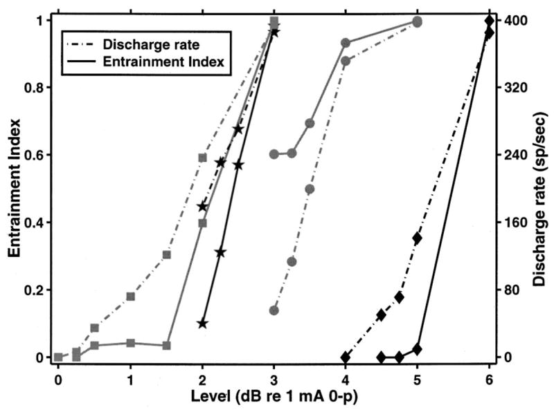
Entrainment index (solid line) and discharge rate (dashed line) as a function of stimulus level for four units from the same animal. Entrainment index is defined as the ratio of intervals that fall between 1/2 and 3/2 of the stimulus period to the total number of intervals. An entrainment index of 1 represents perfect entrainment. At the highest levels, all four fibers entrain to the stimulus. This entrainment does not occur in a healthy ear in response to pure tones. At stimulus levels below those that evoke discharge rates of 200 spikes/s, the entrainment index is 0 for two units, indicating that the mode at the stimulus period is missing in the units’ responses. In contrast, responses to pure tones in a healthy ear have entrainment indices between 0.6 and 0.9 (Joris et al., 1994).

2. Small modulation depth

Figure 12 shows average discharge rate and response modulation depth (which is a measure of modulation of the period histogram, and is twice the synchronization index) for a single unit as a function of level. The stimulus was a 250 ms pulse train (4.8 kpps) that was modulated by a 400 Hz sinusoid in the last 100 ms (modulation depth 1%). Average discharge rate increased three-fold over the 1.5 dB range of levels. In contrast, response modulation depth was nearly constant at 0.7–0.8 for all levels, indicating robust phase locking. The first mode in the interval histogram shifts to the left as the level increased, reflecting the increase in average rate (lower panels). While the first mode is a multiple of the modulator period at the lowest and at the highest level shown, at the intermediate level of 4.75 dB re: 1 mA, it falls nearly halfway between the first and the second multiple of modulator period (arrow). This result suggests that at this level, the first mode is not related to the modulator frequency. We hypothesize that for the higher levels, the first mode is related to the preferred firing periods demonstrated earlier for high-frequency unmodulated stimuli. To test this hypothesis, we computed IHs from responses that immediately precede the modulation onset (gray line). As predicted by the hypothesis, the location of the mode of the IH for these responses roughly matches the mode observed during the modulated segment at levels above 4.75 dB re 1 mA. At the lower level, however, the first mode of the modulated segment differs from the first mode of the pre-modulation responses and is related to the modulation frequency.

FIG. 12.

Responses of a unit to a stimulus with modulation depth of 1%, modulation frequency of 400 Hz, at several levels. The top panel shows both the response rate and the modulation depth of the response as a function of level. Both the response rate and the response modulation depth are computed during the modulated portion of the stimulus. Note that the modulation depth of the response is nearly independent of level. The lower panels show the IHs computed from the responses at three different levels. The solid areas represent the IH computed from responses during the modulated portion of the stimulus while the gray lines are the IHs computed from responses preceding the modulation. At the lowest level, the mode of the IH for the modulated portion is related to the modulation frequency. At the higher levels, however, the mode of the IH for the modulated portion is similar to the mode described earlier for the unmodulated responses and not to the modulation frequency.

Thus, for very low modulation depths, interval histograms can differ from IHs evoked by acoustic tones because their IHs can include modes that are not multiples of the modulator period.

IV. DISCUSSION

A. Adaptation

The adaptation that we report here is generally consistent with previous studies of electrically stimulated ANFs (Moxon, 1967; van den Honert and Stypulkowski, 1987; Javel et al., 1987; Dynes and Delgutte, 1992; Killian, 1994). The result that at least short-term (<150 ms) adaptation depends on pulse rate of the electric stimulus is new. This result may have important consequences for models of electrically stimulated ANFs.

Our working hypothesis is that the slow decrease in discharge rate over time is evidence either of depletion of an “excitatory” agent or accumulation of an “inhibitory” agent. For example, intracellular sodium and extracellular potassium might be the relevant agents for the electrically stimulated ANFs. The changes in the concentrations of these substances may occur because of change in the membrane conductance resulting from the increased spike activity induced by the electric stimulus. Alternatively, concentrations may change even without increased spike activity because the electric stimulus can induce voltage changes across the neural membrane that do not lead to spikes. If the increased activity itself were the primary influence on accumulation or depletion of the agent, we would expect that adaptation would depend primarily on the initial response rate and not on the pulse rate of the electric stimulus. We showed that adaptation of ANFs to electric stimulation depends not only on the initial rate, but also on stimulation frequency. This implies that significantly more agent is depleted due to voltage changes across the membrane that do not lead to spikes during the higher-frequency stimulus. Whether neurons will be able to readjust to the new homeostatic balance if the high-frequency DPT is presented continuously is a topic for future investigations.

B. Temporal response patterns to unmodulated pulse trains

We found that the detailed response pattern of auditory nerve fibers to electric pulse trains also depends strongly on stimulation rate. In particular, while the envelope of the IH of responses to a 1.2 kpps pulse train is nearly exponential, the envelope can strongly differ from an exponential for pulse rates above 4.8 kpps. This conclusion is consistent with published data. Van den Honert and Stypulkowski (1987) described ANF responses to moderate-level electric sinusoids with frequencies between 100 and 1000 Hz. The interval histograms in these data appear exponential. IHs reported for responses to low-rate (<2000 pps) pulse trains appear exponential as well (Javel et al., 1987). Dynes and Delgutte found Gaussian-like interval histograms of responses of ANFs to electric sinusoids for frequencies above 4 kHz (Dynes and Delgutte, 1992). The mode of their IHs is at about 5–6 ms, as in our data. Unfortunately, they do not report IHs for responses with discharge rates below 200 spikes/s, where the tail may be more apparent.

C. Does the response to a desynchronizing pulse train (DPT) resemble spontaneous activity?

Rubinstein et al. (1999) suggested introducing a continuous pulse train into CI strategies to produce neural responses resembling normal spontaneous activity. Our results indicate that if the level of the DPT can be adjusted for each fiber, the responses to sustained high-frequency pulse trains resemble spontaneous activity in some, but not all respects. The variability across stimulus presentations is comparable with that expected for spontaneous activity. For a relatively low pulse rate (1.2 kpps) the envelope of interval histograms resembles those for spontaneous activity for most units. However, for higher-rates (4.8 kpps and above) interval histograms can clearly deviate from those for spontaneous activity, showing a sharp mode that is followed by a long tail. On the other hand, a DPT with a low pulse rate may introduce psychophysically significant periodicity in neural responses that is related to the DPT period. Thus, intermediate pulse rates (above 1.2 and below 4.8 kpps) may be optimal for imitating spontaneous activity.

A further difficulty with the DPT idea is that electrically stimulated fibers respond with discharge rates that are appropriate for spontaneously responding neurons in a healthy ear only over a narrow range of stimulus levels. The small dynamic range reported in this study is consistent with earlier reports of responses of ANFs to electric pulse trains (Javel et al., 1987; Parkins, 1989). Fibers can differ in threshold by 10 dB or more at a single cochlear location near the stimulating electrode (van den Honert and Stypulkowski, 1984). If a DPT is presented at a level that stimulates a large percentage of the fibers, most fibers will respond at rates that are higher than the rates appropriate for producing spontaneouslike responses.

While the differences in DPT sensitivity across fibers are large compared to the level range producing spontaneouslike responses, the DPT idea should not necessarily be ruled out based on the results of this study of short-term (less than 250 ms) stimulation. Electric responses are known to adapt over a course of minutes (Moxon, 1967; Killian, 1994). This longer adaptation may selectively decrease the response discharge rates of fibers with low thresholds to the DPT.

D. Does a high-frequency DPT help encode modulation frequency?

We showed that a modulated pulse train with low (<10%) modulation depth can produce interspike and period histograms resembling responses to tones in intact ears. If we interpret those stimuli as consisting of a DPT plus a highly modulated signal, this result suggests that realistic responses to sinusoidal stimuli might be obtained with a DPT. However, the realistic, tonelike responses are only observed over a narrow range of stimulus levels. Furthermore, for very low (1%) modulation depths, there can be preferred intervals unrelated to the modulation frequency which may be confusing to the central processor. Interestingly, these intervals may co-exist with a high level of phase locking to the modulator frequency.

E. Implications for mechanisms

Our results with unmodulated and modulated stimuli also pose important questions for models of ANF responses to electric stimulation. Published reports based on biophysical models have not described the complex shape of interval histograms (a pronounced mode with a long tail) we observed in responses to high-frequency pulse trains (e.g., Rubinstein et al., 1999). In evaluating mechanisms that may account for this discrepancy it is important to determine whether the relevant processes occur on an interval-by-interval basis or on a slower time scale (e.g., bursting). In a limited number of units for which sufficient data are available, we failed to detect a correlation between consecutive intervals. Thus, the relevant processes appear to occur on an interval-by-interval basis.

Responses that are qualitatively similar to the ones that we report for cat ANFs, in which rapid firing randomly alternates with longer pauses, have also been observed in the squid giant axon that is stimulated by a dc current injection (Guttman and Barnhill, 1970; Guttman et al., 1980). The mechanism for these responses may be similar to the mechanism responsible for the nonexponential responses reported here. A biophysical model that has Hodgkin–Huxley channel dynamics, and that explicitly models random channel noise can account for the observed responses in that preparation (Schneidman et al., 1998). Therefore, it is possible that a biophysical model of ANFs that correctly captures ANF channel dynamics and that explicitly models channel noise may predict the responses that we observed as well.

Although high-frequency pulses used in this paper differ from dc injections used in the study of the squid giant axon, some parallels may exist between the responses evoked by both. In particular, rectification and low pass filtering, both of which are known to occur in neural membrane, may transform the extracellular pulse train into an intracellular stimulus with a significant dc component. Intracellular recordings near the site of excitation are necessary to determine mechanisms underlying the observed responses.

Another intriguing observation is the increase in average discharge rate after the “down” modulation is turned on. The increase in average discharge rate is surprising because the rms stimulus current actually decreases at the onset of the modulator. To our knowledge, such an increased response to modulation has not been reported for biophysical models. Our simulations using the Hodgkin–Huxley (HH) model indicate that an increased response rate can be observed at the onset of the “down” modulation of a high-frequency carrier (Fig. 13), although the model does not mimic the data quantitatively.

FIG. 13.

Response of a current-clamped Hodgkin–Huxley model to a high-frequency sinusoid that is modulated in the last 50 ms of the 100 ms stimulus (bottom). Parameters for this model are summarized in Weiss (1996), p. 191. Simulation temperature was 6.3 °C. The model was implemented in MATLAB and simulated numerically using a 5 μs step. The stimulus was presented as intracellular current injections. The carrier was a 2 kHz sinusoid (400 μA/cm² 0-peak) that was modulated “down” (sinusoidal 50% modulation, 100 Hz modulation frequency). This stimulus was chosen to represent the modulated pulse trains that were used in the physiological study. However, both the shape of the “pulse” and the carrier frequency were adjusted to account for the slower dynamics of the Hodgkin–Huxley model. The time course of the membrane voltage is shown by the gray line. The membrane voltage is shown relative to its resting state. We also show the time course of the membrane voltage averaged over a period of the sinusoidal carrier (dark line). The unmodulated response can be characterized by a single response at the stimulus onset. However, when down modulation is added, the model responds in a sustained manner to every second modulation cycle.

One difference between the HH model and the data is that the HH model exhibits an onset-only response to the sustained high-frequency stimulus. It is unknown whether introducing channel noise into the model would improve the fit between the model and the data. While the Frankenhaeuser–Huxley model (Frankenhaeuser and Huxley, 1964) of the frog sciatic nerve predicts the sustained response during the high-frequency stimulus, it does not show an increase of firing rate at the onset of the down-modulation (personal observations). Future modeling studies would also be needed to determine whether mammalian-based models produce responses to modulated stimuli that more closely resemble our data for ANFs.

F. Implications for the cochlear implant processor

The purpose for introducing a DPT is to improve the coding of modulation in auditory nerve responses. Some aspects of our data appear promising in that respect. A DPT can produce responses that are desynchronized across trials, suggesting that the responses may also be desynchronized across different fibers, as occurs for normal spontaneous activity (Johnson and Kiang, 1976). Desynchronization of auditory nerve responses may lead to an improved temporal coding of stimuli with rapid onsets and high frequencies. For low pulse rates of 1.2 kpps, responses to a DPT imitate some characteristics of spontaneous activity. Over a range of levels and modulation depths, a DPT can help provide temporal discharge patterns for amplitude-modulated stimuli that resemble responses to tones. Other aspects of the data are less promising. For example, we found that DPTs that accurately encode sinusoidal waveforms in the period histogram can show modes in the interval histogram that are not related to the modulator frequency. In addition, for some modulation frequencies and levels, the mode of the interspike distribution that corresponds to the stimulus period can be entirely absent in the interval histogram of the response. It appears, therefore, that successful use of a DPT depends on what exact aspects of the temporal discharge pattern (e.g., intervals versus cross-fiber synchrony) are most important to the central processor for extracting information about the stimulus. Because the exact mechanisms used by the central processor are not known, it is difficult to predict whether adding the DPT will result in an overall improvement in the reception of speech by cochlear implant users.

APPENDIX

The interval histogram exponential shape factor (IH-ExpSF) is defined as the ratio of the error in the fit of the IH with the piecewise, three exponential function to the error of the fit with a single exponential. First, a number drawn from a uniform distribution from 0 to 0.832 ms was added to each interval to eliminate the effect of locking to the 1.28 kHz pulse frequency. Next, the mode of the interval distribution was estimated. Intervals that were longer than the mode were considered to constitute the tail and were included in the analysis; the remaining intervals were discarded.

Next, the IH was recomputed based on the remaining intervals. Instead of computing the interval histograms with a fixed bin size, however, we changed the bin size from bin to bin, such that exactly five intervals fell into each bin. This normalization is convenient because the coefficient of variation of the interval histogram for any given bin is proportional to the number of values that fall into that bin (Johnson, 1996). By normalizing the interval histogram in this way, one achieves equal coefficient of variation in each of the bins. Finally, a logarithmic transformation was applied to the IH so that straight-line fits generated exponential fitting function.

The resulting logarithmic histogram was fit by a linear and by a piecewise linear function by minimizing the least squares error. The piecewise linear function was constrained to be continuous. The times at which the function changed its slope were chosen such that each segment covered an equal number of bins.

To estimate IH-ExpSF distribution expected from a Poisson-with-dead time model, the IH-ExpSF was computed for 1000 interval histograms, each histogram composed of 200 independent “intervals” drawn from an exponential with dead time distribution (dead time of 3 ms). 99% of the generated data fell between 0.68 and 1. This boundary was nearly independent of the event rates of the simulated distribution for rates of 50 to 250 events/s.

References

- Dynes SB, Delgutte B. Phase-locking of auditory-nerve discharges to sinusoidal electric stimulation of the cochlea. Hear Res. 1992;58:79–90. doi: 10.1016/0378-5955(92)90011-b. [DOI] [PubMed] [Google Scholar]
- Efron B, Tibshirani R. An Introduction to the Bootstrap. Chapman & Hall; New York: 1993. [Google Scholar]
- Frankenhaeuser B, Huxley AF. The action potential in the myelinated nerve fibre of xenopus laevis as computed on the basis of voltage clamp data. J Physiol (London) 1964;171:302–315. doi: 10.1113/jphysiol.1964.sp007378. [DOI] [PMC free article] [PubMed] [Google Scholar]
- Guttman R, Barnhill R. Oscillation and repetitive firing in squid axons. Comparison of experiments with computations. J Gen Physiol. 1970;55:104–118. doi: 10.1085/jgp.55.1.104. [DOI] [PMC free article] [PubMed] [Google Scholar]
- Guttman R, Lewis S, Rinzel J. Control of repetitive firing in squid axon membrane as a model for a neuroneoscillator. J Physiol (London) 1980;305:377–395. doi: 10.1113/jphysiol.1980.sp013370. [DOI] [PMC free article] [PubMed] [Google Scholar]
- Javel E, Tong YC, Shepherd RK, Clark GM. Responses of cat auditory nerve fibers to biphasic electrical current pulses. Ann Otol Rhinol Laryngol. 1987;96:26–30. [Google Scholar]
- Johnson DH. Point process models of single-neuron discharges. J Comput Neurosci. 1996;3:275–299. doi: 10.1007/BF00161089. [DOI] [PubMed] [Google Scholar]
- Johnson DH, Kiang NYS. Analysis of discharges recorded simultaneously from pairs of auditory nerve fibers. Biophys J. 1976;16:719–734. doi: 10.1016/S0006-3495(76)85724-4. [DOI] [PMC free article] [PubMed] [Google Scholar]
- Joris PX, Carney LH, Smith PH, Yin TC. Enhancement of neural synchronization in the anteroventral cochlear nucleus. I.Responses to tones at the characteristic frequency. J Neurophysiol. 1994;71:1022–1036. doi: 10.1152/jn.1994.71.3.1022. [DOI] [PubMed] [Google Scholar]
- Kelly OE, Johnson DH, Delgutte B, Cariani P. Fractal noise strength in auditory-nerve fiber recordings. J Acoust Soc Am. 1996;99:2210–2220. doi: 10.1121/1.415409. [DOI] [PubMed] [Google Scholar]
- Kiang NYS, Watanabe T, Thomas EC, Clark LF. Discharge Patterns of Single Fibers in the Cat’s Auditory Nerve. The MIT Press; Cambridge, MA: 1965. [Google Scholar]
- Killian MJP. PhD thesis. University of Utrecht; Utrecht: 1994. Excitability of the electrically stimulated auditory nerve. [Google Scholar]
- Liberman MC. Auditory-nerve response from cats raised in a low-noise chamber. J Acoust Soc Am. 1978;63:442–455. doi: 10.1121/1.381736. [DOI] [PubMed] [Google Scholar]
- McKinney MF, Delgutte B. Correlates of the subjective octave in auditory-nerve fiber responses: Effect of phase-locking and refractoriness. Abstract, Midwinter Meeting of the Association for Research in Otolaryngology; Florida. 1998. [Google Scholar]
- Moxon EC. PhD Thesis. MIT; Cambridge, MA: 1967. Electric stimulation of the cat’s cochlea: A study of discharge rates in single auditory nerve fibers. [Google Scholar]
- Moxon EC. Neural and mechanical responses to electrical stimulation of the cat’s inner ear. MIT; Cambridge: 1971. [Google Scholar]
- Parkins CW. Temporal response patterns of auditory nerve fibers to electrical stimulation in deafened squirrel monkeys. Hear Res. 1989;41:137–168. doi: 10.1016/0378-5955(89)90007-5. [DOI] [PubMed] [Google Scholar]
- Rose JE, Brugge JR, Anderson DJ, Hind JE. Phase-locked response to low-frequency tones in single auditory nerve fibers of the squirrel monkey. J Neurophysiol. 1967;30:769–793. doi: 10.1152/jn.1967.30.4.769. [DOI] [PubMed] [Google Scholar]
- Rubinstein JT, Wilson BS, Finley CC, Abbas PJ. Pseudospontaneous activity: stochastic independence of auditory nerve fibers with electrical stimulation. Hear Res. 1999;127:108–118. doi: 10.1016/s0378-5955(98)00185-3. [DOI] [PubMed] [Google Scholar]
- Schneidman E, Freedman B, Segev I. Ion channel stochasticity may be critical in determining the reliability and precision of spike timing. Neural Comput. 1998;10:1679–1703. doi: 10.1162/089976698300017089. [DOI] [PubMed] [Google Scholar]
- Shannon RV. Temporal modulation transfer functions in patients with cochlear implants. J Acoust Soc Am. 1992;91:2156–2164. doi: 10.1121/1.403807. [DOI] [PubMed] [Google Scholar]
- Shepherd RK, Javel E. Electrical stimulation of the auditory nerve. I Correlation of physiological responses with cochlear status. Hear Res. 1997;108:112–144. doi: 10.1016/s0378-5955(97)00046-4. [DOI] [PubMed] [Google Scholar]
- Teich MC, Khanna SM. Pulse-number distribution for the neural spike train in the cat’s auditory nerve. J Acoust Soc Am. 1985;77:1110–1128. doi: 10.1121/1.392176. [DOI] [PubMed] [Google Scholar]
- van den Honert C, Stypulkowski PH. Physiological properties of the electrically stimulated auditory nerve. II Single fiber recordings. Hear Res. 1984;14:225–243. doi: 10.1016/0378-5955(84)90052-2. [DOI] [PubMed] [Google Scholar]
- van den Honert C, Stypulkowski PH. Temporal response patterns of single auditory nerve fibers elicited by periodic electrical stimuli. Hear Res. 1987;29:207–222. doi: 10.1016/0378-5955(87)90168-7. [DOI] [PubMed] [Google Scholar]
- Weiss TF. Cellular Biophysics. MIT Press; Boston, MA: 1996. [Google Scholar]
- Wilson B, Finley CC, Lawson DT, Zebri M. Temporal representations with cochlear implants. American Journal of Otology. 1997;18:S30–S34. [PubMed] [Google Scholar]
- Wilson BS, Finley CC, Lawson DT, Wolford RD, Eddington DK, Rabinowitz WM. Better speech recognition with cochlear implants. Nature (London) 1991;352:236–238. doi: 10.1038/352236a0. [DOI] [PubMed] [Google Scholar]
- Xu SA, Shepherd RK, Chen Y, Clark GM. Profound hearing loss in the cat following the single co-administration of kanamycin and ethacrynic acid. Hear Res. 1993;70:205–215. doi: 10.1016/0378-5955(93)90159-x. [DOI] [PubMed] [Google Scholar]