Left Ventricle Volume Measurements in Cardiac Micro-CT

Abstract

Micro-CT based cardiac function estimation in small animals requires measurement of left ventricle (LV) volume at multiple time points during the cardiac cycle. Measurement accuracy depends on the image resolution, its signal and noise properties, and the analysis procedure. This work compares the accuracy of the Otsu thresholding and a region sampled binary mixture approach, for live mouse LV volume measurement using 100 micron resolution datasets. We evaluate both analysis methods after varying the volume of injected contrast agent and the number of projections used for CT reconstruction with a goal of permitting reduced levels of both x-ray and contrast agent doses.

Introduction

Cardiac studies in small animals are very challenging. The small size (∼0.1 g and 7 mm long axis) and extremely high rates (∼600 beats/min) of murine hearts under physiological conditions have made in vivo studies of murine cardiac metabolism, function, and morphology difficult.

Although in vivo open chest models of transgenic mouse cardiac function have been proposed[1], non-invasive in vivo imaging has several obvious advantages. Ultrasound echocardiography has been used extensively to phenotype the cardiovascular system in a variety of genetic mouse models[2]. Although echocardiography has been the most widely used method to estimate cardiac function, its results are very operator-dependent. Moreover, echocardiography uses model-based estimation that relies on geometric assumptions that work well only in normal hearts[3, 4]. Alternatively, MR microscopy (MRM) has been applied to assess both cardiac morphology and function in rodents[5-9]. However, neither MRM nor echocardiography offer isotropic resolution, with slice thickness equal to in-plane resolution. All imaging modalities provide data for the measurement of left ventricular (LV) volumes at different points of the cardiac cycle, based on which one can assess cardiac function via ejection fraction, cardiac output and/or wall dynamics.

We have proposed the first micro-CT based method appropriate for in vivo characterization of cardiac structure and function in mice[10], where true 4D datasets are collected with an isotropic spatial resolution of 100 microns and a temporal resolution of 10 ms during the cardiac cycle. We have shown that cardiac micro-CT with a combination of high flux x-ray tube, careful physiologic gating, and the use of blood pool contrast agents can produce image sets with 10-50 times higher spatial resolution than has been seen with in vivo MR[7, 11]. Recently Drangova et al [12] have introduced a retrospective based cardiac micro-CT method that allows a spatial resolution of 150 microns.

The two major disadvantages of cardiac micro-CT are: 1) a significant radiation dose and 2) a large volume of blood pool contrast agent used during a study. The radiation dose required for 10 imaging sets sampling the cardiac cycle at 10 ms temporal resolution is ∼1.5 Gy[10]. This is 1/4 to 1/3 of the mouse lethal dose that ranges from 5.0 to 7.6 Gy[13]. Various approaches have been used in clinical CT to reduce dose such as alternate beam filtering[14], digital filtering[15], tailoring technique to patient size [16-18] or beam modulation according to cross-sectional shape of the patient [19-26]. However, one of the most direct approaches to dose reduction in CT imaging is to use fewer projections, i.e. angular under-sampling. Unfortunately, this also results in increased noise and reconstruction artifacts.

Since the x-ray attenuation of blood and myocardium are similar, contrast agents are essential for obtaining high quality micro-CT images. The suggested dose, 0.5ml /25 g mouse, of the Fenestra VC blood pool contrast agent (ART Advanced Research Technologies Inc. Saint-Laurent, Quebec, Canada) may be large enough to affect the hemodynamics since it represents approximately 1/3 of the total blood volume. Reduction of contrast agent dose is desired but this lowers the contrast between myocardium and blood and is therefore expected to reduce the accuracy of LV volume measurements.

Because reductions of both radiation dose (i.e. number of projections in this study) and volume of contrast agent decrease the quality of micro-CT datasets we are motivated to examine data analysis techniques that can tolerate these quality reductions yet still recover accurate volume measurements. Therefore we test the limits and tradeoffs of radiation and contrast reductions on two different analysis methods. These are: 1) a classical technique based on Otsu’s method[27], and 2) our proposed region sampling within binary mixture method.

Our aim in the present work is to find the minimum image quality, and hence required radiation and contrast agent levels, for cardiac micro-CT that allows accurate LV volumetric estimation. The goal is less than 5% volume error, similar to what is proposed in human cardiac CT [28].

Also, it would be very beneficial to provide directly computed error estimates on a case-by-case basis rather than only relating error estimation to a body of historical experience from a particular tool.

Materials and Methods

Animal preparation

All animal studies were conducted under a protocol approved by the Duke University Institutional Animal Care and Use Committee. A 25 g C57BL/6 mouse was anesthetized with ketamine (115mg/kg, 20mg/ml, 0.17 ml) and diazepan (27 mg/kg, 0.5 mg/ml 0.16 ml) and peroraly intubated for mechanical ventilation using a ventilator [29] developed in-house, at a rate of 90 breaths/min with a tidal volume of 0.4 ml. A solid-state pressure transducer on the breathing valve measured airway pressure and electrodes (Blue Sensor, Medicotest, UK) taped to the animal footpads acquired the ECG signal. Both signals were processed with Coulbourn modules (Coulbourn Instruments, Allentown, PA) and displayed on a computer monitor using a custom-written LabVIEW application (National Instruments, Austin, TX). Body temperature was recorded using a rectal thermistor and maintained at 36.5° C by an infrared lamp and feedback controller system (Digi-Sense®, Cole Parmer, Chicago, IL). A catheter was inserted following a tail vein cut down and used for injection of the contrast agent. Animals were placed in a cradle and scanned in a vertical position. During imaging, anesthesia was maintained with ketamine (0.04 ml) delivered IP every 30 min.

The scanning time for a complete 3D dataset with most currently available micro-CT systems is ∼6 to 12 minutes. Thus micro-CT imaging with a single bolus injection of conventional contrast agent as used with humans in the clinical arena is not possible. Fortunately, a new class of blood pool contrast agent for micro-CT [30, 31] with prolonged vascular residence time is now available.

This contrast agent, Fenestra™ VC (ART Advanced Research Technologies, Saint-Laurent, Quebec, Canada), contains iodine at 50 mg/ml concentration. When used in a dose up to 0.5ml/25 g mouse, as recommended by the manufacturer, it has been shown to provide excellent contrast (∼500 HU difference between blood and muscle) that facilitates quantitative measurement of LV volume [32]. In this work we scanned the same animal four times with each scan taking place 5 minutes after successive intravenous injections of 0.125 ml of Fenestra™ VC. Therefore the four scans were performed at four different levels of contrast agent volume corresponding to (0.125, 0.25, 0.375, 0.5) ml /25 g mouse. The resulting datasets allow us to examine the influence of contrast agent dose on image quality for LV volume estimation using several analysis techniques.

Image acquisition

We used a prototype cone beam micro-CT system with a design that addresses two of the most significant barriers to micro-CT in small-animals —the reduced signal-to-noise imposed by smaller voxels and motion[33]. As one reduces voxel size, the x-ray dose must be simultaneously increased to maintain the voxel signal-to-noise-ratio (SNR)[13]. The most direct approach to increasing SNR is to increase total fluence rate. It is not possible to significantly increase the fluence rate of most commercial micro-CT systems in current use[34-36], since these systems use smaller fixed focal spot x-ray tubes. One can integrate over extended periods with these devices, but then biological motion poses the resolution limit. Our system allows the use of high flux x-ray tubes that are 250-times brighter than the tubes in commercial micro-CT systems[33]. Moreover the system takes advantage of integrated physiologic monitoring and control of breathing and cardiac motion that has been developed previously for MR imaging of small animals [37] to limit artifacts and motion blur from both respiratory and cardiac motion. Our micro-CT system acquires projected radiographs as the animal is rotated in front of a high-resolution 2D imaging x-ray detector. The detector is a cooled 16-bit CCD camera with a Gd₂O₂S phosphor on a 3:1 fiber optic reducer (X-ray ImageStar, Photonics Science, East Sussex, UK). The camera has a 95 mm² active field of view with an image matrix of 2048×2048 pixels of 46×46 microns. The camera drivers permit flexible readout and rebinning to allow imaging up to 8 frames/sec. For the studies shown here, data were acquired over a whole field of view with binning to produce two-dimensional 1024×1024 projections.

The x-ray settings during scanning were 80 kVp, 200 mA, and 10 ms exposures/projection. Four scans (each 380 projs/190°) were performed on the same animal with the four concentrations of contrast agent discussed previously. All scans used prospective cardio-respiratory gating, i.e. at end expiration and synchronized on the QRS complex. Heart rate was stable during scanning (HR= 440 +- 20 beats/min), due to our ability to maintain physiologic stability by controlling anesthesia and temperature levels.

These four scan sets, representing as nearly as practical the same state of the animal, were used to reconstruct 24 different 3D image arrays (512³) with isotropic 100 micron resolution by using the full 380 projections and 5 angular subsamplings of 190, 126, 95, 75 and 63 projections to retrospectively emulate reduced radiation dose. Reconstruction used a Feldkamp algorithm[38], within a commercial software package (Cobra EXXIM, EXXIM Computing Corp, Livermore, CA). Thus we obtained 24 3D reconstructions covering a range of 4 levels of contrast agent and 6 levels of reconstruction quality. Examples of corresponding axial slices from all 24 reconstructions are shown in Fig. 1. The images are labeled with names from C11 to C46 for easy reference later in this text.

Fig.1.

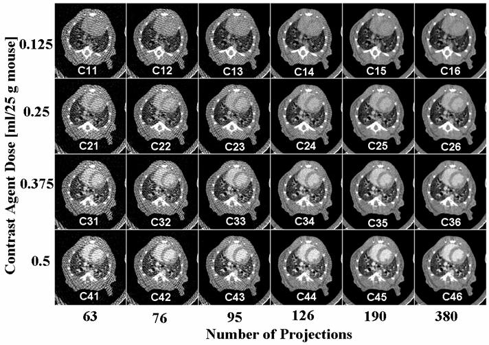
An example of corresponding axial micro-CT slices in 24 datasets for 4 different levels of contrast agent and 6 levels of reconstruction projections. The sets are labeled for further reference. Note that the best image corresponds to maximum contrast dose and maximum number of projections (i.e. C46).

Dosimetric measurements were performed using a Wireless Dosimetry System Mobile MOSFET TN-RD-16, SN 63 B (Thomson/Nielsen, Ottawa, ON, Ca). Five MOSFET dosimeters silicon chips (1mm² active area 0.2mm × 0.2mm) were positioned at the surface and the center of another rodent like phantom made out of acrylic. The radiation dose of mouse micro-CT scanning was estimated from measurements during phantom scans using 380 projections/190° and the same x-ray settings as used for the animal scans.

Image analysis

To illustrate some of the problems associated with the analysis of live mouse micro-CT data, we show a typical in vivo acquired micro-CT image (fig.2A) with 100 micron resolution compared to an ex-vivo MR microscopy image (fig.2 B) at 20 micron resolution. The MR shows that the interior heart wall is not a continuous smooth surface but has fine anatomical detail, the trabeculae carneae, at many scales and some structures, papillary muscles and tendons, cross portions of the blood pool. Even in areas of smooth surfaces a reconstructed voxel grid would not line up with surface boundaries so there are always voxels straddling material boundaries. These partial volume voxels have intensity values composed from material on both sides of the surface. In smooth surface regions this can be used to recover “super-resolution” surface models. In areas of complex structure the partial volume effects cannot be avoided regardless of resolution. Therefore reconstructed ventricle wall data show gradual changes of contrast over a partial volume layer that is thicker than would be produced across a sharp blood/muscle boundary. The intensities of partial volume voxels contain valuable information about the relative quantities of blood and muscle that would produce the observed data. We would like to use that information to improve accuracy. Motion blur causes another kind of partial volume effect. Even though a 10 ms x-ray exposure is short enough to produce good quality stop-motion of the heart there are still times during the cycle when parts of the LV wall move more than 1 voxel during the exposure interval. A blood/myocardium boundary moving through a voxel during the exposure time is recorded as a mixture weighted according to the relative residence time of the materials. This effect is more significant at high resolution but will have little effect on our volume measurement method.

Fig. 2.

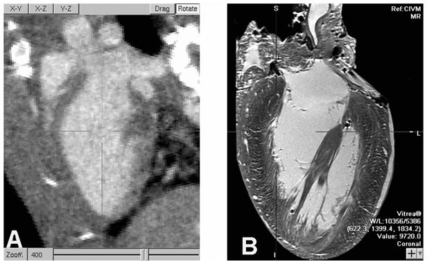
An oblique slice through reconstructed 100 micron/voxel micro-CT from a live mouse, on the left, shows the LV blood highlighted by contrast agent and motion blur suppressed due to 10 ms x-ray pulse width. MRM imaging of a fixed heart at 20 micron resolution, at right, reveals substantial anatomical detail that cannot be resolved in live mouse imaging. High precision measurements of LV blood volumes have to account for these unresolved features. (Note: The micro-CT is digitally zoomed to 400%.)

LV Volumetric measurement can be done in three ways based on: 1) segmentation, 2) histogram analysis and 3) a region sampled mixture model. In practice, each of these methods would be applied within a user defined region of interest (ROI) that targets the LV blood pool and surrounding heart tissue. We present each of these methods and the problems associated with their use with micro-CT data.

A) Segmentation Based Methods

A manual segmentation approach relies on a “seeing is believing” representation of contours drawn through the visual estimate of the lumen outline in 2D slices. These 2D contours, possibly with interpolation, smoothing or fitting to a mathematical shape model, are stacked to form the 3D segmentation. Finally the volume is measured by counting the voxels inside the 3D segmented stack. However, when image quality declines, due to increasing noise or low contrast, the visual feedback required for segmentation may be lost. Furthermore the process is tedious and suffers from subjective manually driven operation and is often only applied to selected slices rather than to an entire volume. There are many techniques for automated and semi-automated segmentation that could be applied to LV volume measurement. These are generally based on either threshold selection or edge detection and can work quite well for high contrast data with low noise levels. We have previously used the region growing segmentation method as implemented for ImageJ (http://rsb.info.nih.gov/ij/) as one freely available plugin called Segmenting Assistant (http://php.iupui.edu/~mmiller3/ImageJ/SegmentingAssistant.html) for this task but find it is only practical for high quality images. In this study, we work with noise and contrast levels that extend beyond the range where visual or automated segmentation methods, especially edge based methods, can operate reliably.

B) Histogram Based Approach

Measurement of LV volume can be done using a statistical histogram approach known as the Otsu method [27] to produce the minimum within class variance partitioning of the voxel histogram. The most general implementation needs to be given the number of classes that it should find and the 1D histogram that should be partitioned. It then returns threshold values that can be used to segment the data into the specified number of low variance classes. Hence, the Otsu method is usually considered to be a segmentation method although it does not always have to be used for that purpose. In the two class case, which is most applicable to our task, the algorithm is often used in computer vision and image processing to perform thresholded reduction of gray scale images to bi-level images such as for separating foreground from background. In that application the image histogram is assumed to be bimodal. The threshold that minimizes the class variances produces the desired, “foreground and background,” bi-level segmentation.

Similarly, our LV measurement application can be considered as bi-level segmentation over a 3D region of voxels containing the LV blood and surrounding heart tissue. The Otsu process eliminates human vision considerations to produce an objective computed result over the selected ROI and it avoids issues of spatial distribution of materials since that information is not part of the histogram.

The count of voxels classified as blood according to the threshold is the Otsu estimate of LV blood volume. A simple way to find the Otsu threshold is to computationally scan the range of possible thresholds and record the value that provides the minimum sum of partition variances. Although most implementations use faster ways to find the threshold even brute force is reasonably quick since it works on a 1D histogram array and only over the constrained range of values that actually occur inside the ROI.

We illustrate some issues associated with histogram methods in Fig 3. The top left (fig.3 A) shows an axial micro-CT slice through the heart and overlaid with manual segmentation (fig.3B) of the relevant voxels into three regions: pure myocardium (blue), pure blood (red), and between (green) i.e. an intermediate unclassified region. The histograms associated with each of these groups as well as the global histogram, which is the sum over all three regions, are shown in Fig.3C. Notice that the pure blood and muscle distributions are well defined highly Gaussian distributions. The widths of the distributions are primarily due to the per voxel noise level with a slight widening of the muscle distribution because that tissue is not quite as uniform as the blood. Because of the point spread function of the micro-CT reconstruction and the complex heart wall structure the unclassified region, which contains the interface of muscle and blood, has an intermediate distribution between the two class means.

Fig. 3.

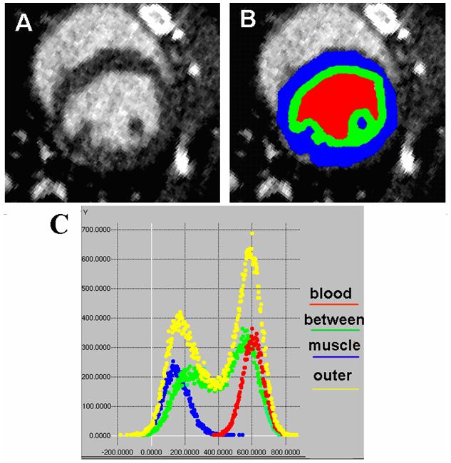
These axial images show micro-CT data (A) and a manual segmentation of the three relevant regions of an ROI slice (B). Red is selected as pure blood, blue as pure muscle and green as an intermediate unclassified transition zone spanning the blood/muscle boundary. The graph in (C) shows the corresponding color-coded histograms captured from the full 3D ROI of a dataset plus a yellow composite histogram of the entire ROI (which is therefore the sum of the blood, between, and muscle histograms).

The Otsu method uses only the composite ROI histogram, yellow in Fig. 3C, to recover a single threshold that is then used to make a forced binary classification of every voxel as either blood or muscle. In this high contrast and low noise example the composite ROI histogram shows a distinct minimum between the muscle and blood peaks. Hence, the resulting threshold should provide a good volume estimate from the count of the blood voxels which, in this case, are above the threshold. However, if contrast is decreased, the blood and muscle peaks will move closer to each other. Furthermore increasing noise will broaden the peaks so the overall distribution eventually looses its bimodal shape and becomes relatively symmetrical around its global mean. Under those conditions, and for any sufficiently symmetric distribution, the Otsu threshold converges to the mean and the accuracy of volume measurement will be lost. In this method the influence of every voxel is the same regardless of whether it is near the threshold or far from it.

C) A Region Sampling Based Approach

Due to limitations of both the segmentation and Otsu methods we have reexamined LV measurement as a two class mixture model. To work with lower contrast and higher noise data, resulting from reductions of contrast agent and number of reconstruction projections, we propose to sample regions of known pure blood and muscle in order to accurately recover their individual means. This additional information, used together with the overall ROI histogram, should permit increased accuracy at higher noise levels and lower contrast. The regions of known blood and muscle can be selected based on anatomical properties of the live heart LV. In particular, except at the valve plane, the LV includes a continuous surrounding heart wall and does not have encroachment of heart tissue into the centermost part of the blood pool.

In this method the final LV volume is computed as a simple function of average x-ray attenuation over a few large groups of voxels. Classification of individual voxels is not involved in the measurement processing. We assume that at all scales, individual voxels or large regions, the average value of a region is simply the average of the individual blood and muscle x-ray attenuations weighted according to their proportions in the region. This assumption is already inherent in the CT reconstruction process. In equation form, this mixture average μ_total over the entire ROI is:

$${\mu }_{\text{total}}={\mathit{Fract}}_{\text{blood}}\cdot {\mu }_{\text{blood}}+{\mathit{Fract}}_{\text{myocardium}}\cdot {\mu }_{\text{myocardium}}$$

where μ_blood and μ_myocardium are the mean attenuations of pure blood and myocardium and Fract_blood and Fract_myocardium are the fractions of blood and myocardium contained within the entire ROI.

Recognizing that Fract_blood + Fract_myocardium = 1 and solving for Fract_blood we obtain:

$${\mathit{Fract}}_{\text{blood}}=({\mu }_{\mathit{ROI}}-{\mu }_{\text{myocardium}})∕({\mu }_{\text{blood}}-{\mu }_{\text{myocardium}})$$

Significantly, Fract_blood does not depend on individual voxels but on the averages of three large groups. This provides great benefit, for both accuracy and for error estimation, by using the standard error of the mean, $\mathit{SEM}=\sigma ∕\sqrt{N}$ where σ is standard deviation of the voxel values and N is the number of voxels. Overall accuracy depends not only on the ROI standard error but also of the pure blood and myocardium sample regions. At 100-micron resolution a typical LV measurement involves ∼20,000 voxels each for the blood and muscle samples and 80,000 to 100,000 in the full ROI. Even if the ROI voxel distribution is non-Gaussian its SEM distribution rapidly becomes Gaussian as N increases. Therefore we can leverage the value of large N and be confident that errors of the means fall into narrow Gaussian distributions and the averages used to compute Fract_blood can be measured with high precision even in the presence of substantial noise. Note that this principal assists volume measurement but not voxel level segmentation.

The error of the final volume result can be estimated by propagating the three SEM distributions through the calculation process. Although there is no known closed form solution for this error propagation case we estimate the final error by independently sampling each of the three SEM distributions by gaussian random number generation, computing a volume from each set of three values, and accumulating the results over a large number of trials. In this work we used 1,000,000 trials which takes ∼1 CPU second so the lack of an algebraic solution is not a restriction in practice.

Conceptually, this measurement technique is similar to calculating the quantities of two known density substances from the weight of a measured volume of their mixture. In this case the mixture consists of the entire LV blood pool and a surrounding layer of myocardium. Rather than segmenting blood from muscle we are computing the relative fraction of blood and muscle directly from all of the voxel intensity values as aggregated into the 3 group means. Unlike the Otsu method this mixture analysis inherently applies a natural weighing of the “analog” value of every voxel according to the overall statistical distribution. This method replaces complications of segmentation by a simple ratio and simultaneously addresses partial volume effects, sub-resolution detail, residual motion blur, and low signal to noise ratio (SNR). All of these factors, which are problems for segmentation, involve the mixing of information from both blood and muscle (see Fig.3). Outside of the selected samples of blood and muscle there is no additional assumption about the spatial distribution of blood and muscle in the unclassified region.

In practical terms, ROIs are built manually using PSC-VB’s (http://www.nrbsc.org/vb/index.php) volume carving tool (see Fig.4). Each ROI basket consists of a few, typically 5 to 10, rough outlines through short axis cuts of the LV (Fig.4A). The process starts with manual placement of the valve plane, shown in side views in (Fig.4B) and (Fig.4C), for the first outline which is at the top left in Fig. 4D. The valve plane is tilted with respect to the body and, in our process, is treated as a logical flat end to close off the ROI at the top of the LV (Fig.4 D). Users navigate progressively along the long heart axis to manually place new 12-point outlines as needed to generate a 3D ROI basket surface that stays inside the LV heart wall and entirely contains the LV blood pool. At each step any or all of the control points may be adjusted to keep the outline shape inside the myocardium. This is not difficult since the heart wall is ∼8 voxels thick and precise user placement is not needed except for the tilt and location of the valve plane itself. Specimen voxels outside of the ROI, based on an all or nothing decision with respect to the interpolated basket surface location, are not part of any further analysis. The “pure” muscle voxels are sampled from a thin layer immediately inside the ROI surface. A smaller ROI is built in the center of the LV blood pool as a sample of “pure” blood (Fig.4 E). Internal to the computation the set of 12-point outlines represent 3D geometric surfaces shown in (Fig. 4 D+E) and ultimately form a set of 3D “voxel masks” marking the three voxel groups used for LV volume measurement. The test ROI voxel masks used for this work contain 16110 muscle, 20278 blood, and 50706 unclassified voxels for a full ROI volume of 87094 voxels. (Due to 100 micron CT reconstruction there are 1000 voxels/ul). Fig.4F shows a cut plane through blood and muscle masks (black and white respectively). For simplicity during development we export the masks and ROI voxels to external C programs rather than doing the entire process inside of PSC-VB. We plan to put the fully tested and debugged code into PSC-VB for future public release.

Fig 4.

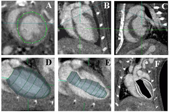
A typical ROI basket is built by drawing outlines in short axis images (A). It is defined by only a few curves and its entire surface is inside the myocardium except at the valve plane. The valve plane, shown as the blue line in coronal (B) and sagittal (C) planes, is treated as a flat end to close the ROI volume enclosed by the basket (D). Image (E) shows a smaller ROI built to sample “pure” blood. Image (F) slices through the 3D regions produced by nesting the two ROIs that are used to measure mean values for “pure” blood and muscle, marked black and white respectively, as discussed in the text. Note: The Z axis as discussed for ROI shift tests is vertical in B, C and F.

The time required to create the ROI basket is about 4 min. Once a user creates a basket corresponding to a single 3D set acquired for a single point in the cardiac cycle, the same basket can be used with adjustments for other data volumes acquired at different points in the cardiac cycle. Thus a whole cine micro-CT 4D dataset can be analyzed and a LV Volume-Time curve can be created.

We used both the Otsu method and the region sampling method to estimate the LV volume for all 24 micro-CT datasets, 4 variations of contrast agent times 6 variations of reconstruction projections, using the same ROI. That ROI was initially built using the highest quality C46 dataset and was uniformly applied to all of the datasets so that we could isolate variations due to contrast, number of projections and analysis processing from variations in ROI targeting. Because the Otsu process only uses histogram data it was run using histograms of the full 87094 voxel ROI volume (Fig. 4D) in order to exactly match the volume processed by our region sampling method.

Because analyses ultimately depend on the particular voxels that are analyzed we also tested the sensitivity of LV volume measurements across ROI targeting variations. This was done by repeating the volume measurements using the same test ROI but with shifts over the range [-4, 4] voxels along the three data axes. Because the heart wall is ∼8 voxels thick this range of 9 shift positions on each axis approximates the range of position variations that we expect in practice. The same shift tests were done for the highest and lowest quality dataset, i.e. C46, C11. We did not run shift tests with the Otsu method.

Results

During micro-CT scanning using 380 projections acquired over 190° at 80 kVp, 200mA and 10ms per exposure, the measured dose was ∼28.71cGy and the elapsed imaging time was 12 minutes. By reducing the number of views the imaging time and the radiation dose are linearly reduced. Thus, for (380, 190, 126, 95, 75, 63) projections the imaging times per 3D volume are approximately (12, 6, 4, 3, 2.4, 2) minutes and the radiation dose is (28.71, 14.35, 9.57, 7.17, 5.74, 4.78) cGy.

Fig.1 shows the increase of artifacts and noise as the number of projections is decreased. To quantify this, Fig. 5A presents the dependency between number of projections used during reconstruction and the noise level (given as the standard deviation) measured in the LV blood and muscle ROI sample regions for the sets with maximum volume of the contrast agent (0.5ml) i.e. the sets C41 to C46. On the same graph we plot the same noise measurements but taken in a water phantom with a diameter of 2 cm using the same scanning and reconstruction parameters as in the mouse experiments. Note that for a sufficient number of projections (190, 380) the noise levels converge to similar values for the mouse and the water phantom. However, as the number of projections is reduced the noise levels in mouse datasets are higher due to streaking artifacts caused by highly attenuating structures such as bones.

Fig.5.

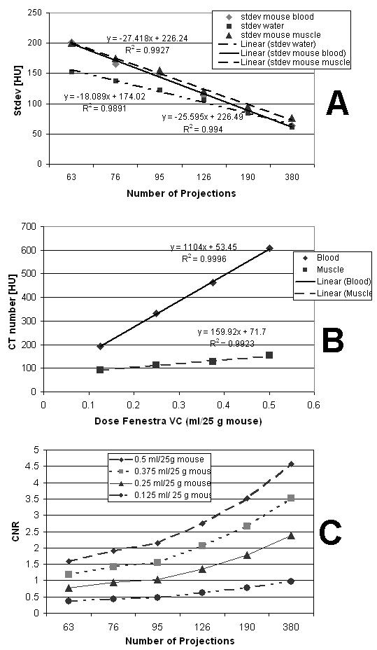
Reconstruction noise as standard deviation for mouse blood, heart muscle, and a water phantom vs. number of projections at 0.5 ml contrast agent (A); The CT attenuations of blood and muscle vs. contrast agent levels at 380 projections (B); The Contrast to Noise Ratio (CNR) computed as described in the text. Note that the usable contrast is the difference between the blood and muscle attenuations shown in (B).

Reductions of contrast agent dose produce less contrast difference between the myocardium and blood. Fig.5B shows a linear increase of attenuation for both the LV blood and myocardium with increasing dose of contrast agent using the 380 projection datasets C16, C26, C36 and C46. Since we used a blood pool contrast agent the muscle (myocardium) shows only a small increase in attenuation with increases of contrast agent. The difference between the blood and the myocardium attenuations is the contrast available for our task (i.e. contrasts from ∼100 to ∼450 HU). As expected higher contrast agent dose results in a more distinct separation between the two materials and would help with measurements of the LV volume especially if these are based on the segmentation or histogram approaches.

Fig.5C shows the combined effects of the noise and contrast agent dose by showing a plot of the contrast to noise ratio (CNR). The CNR was computed as: $\mathit{CNR}=\frac{{\mu }_{\text{blood}}-{\mu }_{\text{muscle}}}{\sqrt{{{\sigma }_{\text{blood}}}^2+{{\sigma }_{\text{muscle}}}^2}}$ where μ_blood and μ_muscle are the mean values in the LV blood and heart muscle samples for the test ROI. CNR is plotted versus the number of projections used for reconstruction at each of the four levels of contrast agent dose.

Fig.6 shows the comparison between the LV volume measurements performed over all 24 datasets using Otsu’s histogram approach and the sampled region method. The two analysis methods provide similar LV volume estimates for high contrast and high number of projections data (see sets C26, C35, C36 and C45, C46). Both methods are able to show small stepwise increases of LV volume with each successive injection of contrast agent. This reinforces the argument that minimal contrast agent is desirable in order to reduce modification of the volume we are trying to measure. (It is not yet clear if the larger jump from the C1X to the C2X sets represents a real signal related to stress response in the animal or whether the natural LV volume may have been even lower.) However as noise increases due to reduced number of projections Otsu’s method produced significantly lower volumes and shows a systematic drift relative to the region sampling method. Because the number of projection cases for each contrast level are from exactly the same heart state (i.e. from a single scan) we know that the Otsu divergence is due to the analysis rather than to any real change of LV volume.

Fig.6.

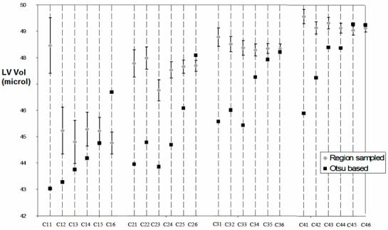
LV Volume estimation in the 24 datasets using sampled regions for blood and myocardium and the Otsu histogram based methods. The error estimation is only possible for the sampled region method.

We note that the computed error estimates, shown as standard deviation bars in Fig 6, are provided as part of the sampled region analysis. Directly computed error estimates are not possible with Otsu’s method. Fig.7 presents the error estimate as a percent of LV volume for a 95% confidence interval (i.e. 1.96 σ) for the region sampling method. Therefore, we are 95% confident that the estimated LV volumes are within ∼4% of the proper values over all but the highest noise case in the lowest contrast set.

Fig.7.

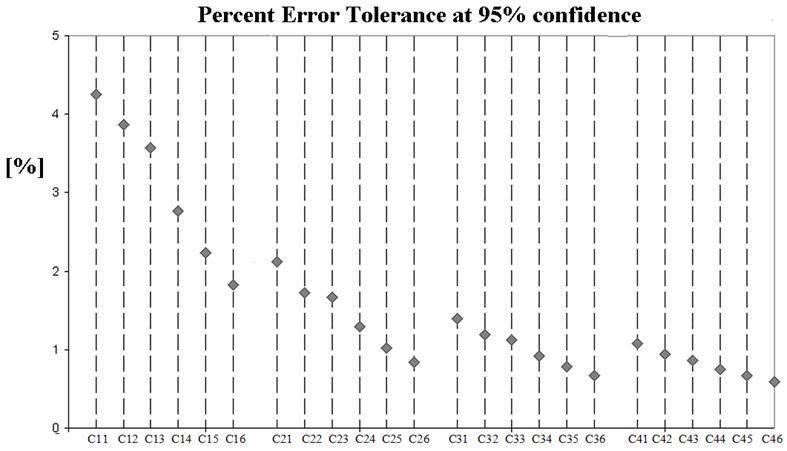
The error tolerance as percent of measured volume for a 95% confidence interval (i.e. 1.96σ) for the sampled region method. We are 95% confident that measured volumes are within ∼4% of the proper value over all but the lowest contrast set.

Fig.8 illustrates the sensitivity of the region sampled method to ROI basket placement with both the lowest (C11) and highest (C46) image quality using shifts of the basket along all three axes.

Fig. 8.

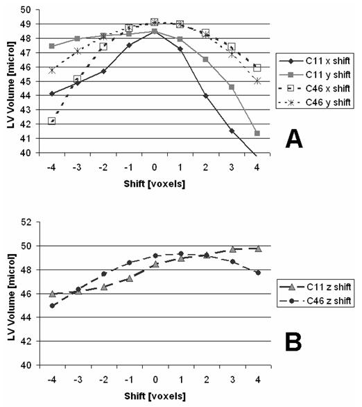
LV Volume variations using region sampling analysis for shifts of the ROI along X-Y axes (A) and Z-axis (B). We show here results for both the lowest (C11) and highest (C46) CNR quality data sets.

Discussion and Conclusions

Segmentation of the LV chamber and its volume estimation using 3D micro-CT data is related to both the image quality, influenced both by the contrast agent dose and the radiation dose, and the image analysis approach. In our case we decouple issues of volume measurement from segmentation by using two non-segmenting methods for volume estimation: the Otsu histogram method and the region sampled mixture method. A visual segmentation based approach would need to fulfill the Rose criterion for visual detectability [39] which requires a detectable contrast difference, CNR, at least 3-5 times greater than the standard deviation, i.e. the noise in the image. Most automated segmentation methods have similar CNR requirements.

But, decreases in contrast agent dose reduce the inherent contrast between blood and muscle while reductions in the number of reconstruction projections reduce image quality by introducing noise and artifacts (see Fig.1 and Fig.5). The graph shown in Fig. 5C illustrates how the CNR changes due to the variation of contrast agent dose and number of projections. In these data the Rose criterion is only reached when a high dose of contrast agent (0.5 ml) is used in combination with a large number of projections, (CNR > 3 only for sets using 190 and 380 projections) or with a 0.375 ml contrast dose and the full 380 projections. None of the other datasets satisfy the Rose criterion and therefore one would not expect a visual segmentation approach to be effective. For the highest quality C46 case we were able obtain a measurement using region growing with the ImageJ Segmenting Assistant plugin. This took ∼10 minutes and gave a volume of 48.803 ul which, in this case, is good agreement with our other results for C46. However, since we seek quantitative LV volume estimates, visual perception is not always necessary. As shown by the plots in Fig. 6 we can estimate LV volume in all cases using either our region sampled mixture approach or by Otsu’s method. As expected these two analyses show similar performance for the highest quality datasets at maximum contrast (C45 to C46) or with less contrast agent but maximum number of projections C26, C36, C46. The results from the region sampling method suggest both precision and accuracy showing variations of less than 2% (see Fig.7) over all but the lowest contrast agent dose. On the other hand Otsu’s method, while showing some tolerance to reduced contrast, fails at high noise levels by showing progressively increasing bias. This is not surprising since reduction of the number of projections or contrast agent dose cause the raw histogram distributions to merge into a single peak and voxel level classification by the Otsu threshold becomes inaccurate. The Otsu bias toward low values is due to threshold drift toward the overall mean which, for a perfectly symmetric distribution, would give a 50% blood volume out of the full ROI. In this case that would be 43.54 microl which is very nearly the Otsu result for the lowest CNR datasets.

One of the sensible aspects of using a ROI-basket to define the analysis regions concerns user variations of ROI placement. For situations with high image quality, i.e. the C46 dataset, the maximum measurement errors due to inaccurate ROI basket placement are less than 14% (see Fig.8A). However, low image quality datasets such as C11 would increase the measurement error to as much as 25% for such cases. Therefore visual image quality to permit manual ROI construction within ∼2 voxels could be significant.

However, the raw shift sensitivity numbers can be misleading since they conceal a simple self centering method that was not applied during the shift tests. Even at the highest noise level, C11, the shape of the error curve is concave downward for shifts of X and Y (see Fig.8A). This is because our recommended basket construction operates like an approximate prior template for the blood/muscle distribution that can be tested around an initial starting position. Therefore a simple search for the local maximum will find the best fit of the ROI basket on the data. This effect can be understood by looking at Fig. 4 B, C & F. Drifts of the template blood and muscle masks will incorrectly sample ROI voxels in way that tends to underestimate the volume relative to the optimal position. Drifts along the Z axis are more difficult. Downward Z drift is still self limiting. Upward motion, however, puts LV blood in the position of other blood above the valve plane but also moves the upper LV wall samples into blood regions. In high CNR (C46) cases the volume maximization search is still effective, though it’s displaced by 1 voxel position from our manual estimates. Eventually the upward Z limit fails at sufficiently poor CNR levels (C11).

In this publication, we are primarily concerned with comparing the numerical effects of contrast and x-ray levels over the same regions of analysis. Therefore, since all of the analysis methods we have considered, (segmentation, Otsu and mixture region sampling) have similar ROI construction and positioning requirements the sensitivity to upward Z drift for high noise cases is not a special limitation of region sampling as compared to the other methods. Also, for the typical application of LV volume estimation as part of a cardiac ejection fraction or other computation that concern the subtraction of two volumes, such as systolic and diastolic, what is most important is to achieve the same placement of the valve plane in the two volumes. Because the diameter of the blood pool adjacent to the valve plane does not change as dramatically as regions lower in the heart small systematic displacements of the analysis valve plane from its preferred anatomical location tend to cancel out during the subtraction operation. Nevertheless, further study of manual ROI construction is warranted in order to examine the effects of operator experience, anatomical knowledge, and other human factors in conjunction with image quality issues. Similar tests of eventual automated ROI construction and placement will be needed but will be easier to carry out.

There is no easy answer regarding the best contrast agent dose and radiation dose that should be used. The relative importance of accuracy, low radiation, or minimal volume of contrast agent will be different depending on specific experimental aims and these in turn affect the cost and speed of data collection. According to Fig.7 and 8 errors less than 4% could be expected with the region sampling method when using all datasets. However, it is not yet proven that users can reliably build and place ROIs in sets containing very limited volume of contrast agent, 0.125 ml, and reconstructed using very few projections i.e. 63 such as set C11. In some circumstances it may be better to reduce x-ray exposure by other means, such as shorter pulses or reduced current, rather than by reducing the number of projections. This is an area of ongoing work that will also evaluate the effects of reconstruction algorithms.

Accepting as much as 5% error, as suggested for human cardiac CT[28], in any of these volumes could bring a maximum error of 7.1 % for stroke volume (SV) as computed by subtraction of diastolic and systolic volumes and adding the variances. This might be not sufficient for studies comparing groups of mice with subtle differences in cardiac function. Therefore, for those cases the image quality has to remain high. If we choose however an image quality equal or superior to set C24 i.e. 126 projections and with a contrast dose of 0.25 ml Fenestra i.e. according to Fig.8 we would be confident that measurement error was less than ∼1.5% with the region sampling method and the image quality would also be sufficient for correct manual ROI-basket placement (see fig.1).

Thus by using 0.25 ml Fenestra the contrast agent dose is reduced to half (0.25 ml vs. 0.5ml) involving a reduced blood volume overload and less influence on the hemodynamics. The associated radiation dose is reduced threefold from 28.7 to 9.5 cGy and scan time from 12 to 4 minutes. Therefore, 10 time points during ECG cycle will require 0.95 Gy and ∼40 minutes scan time.

We also note that contrast agents with a higher iodine concentration would enable more enhancement for the same injected volume. Indeed, in our recent work [40], we used a contrast agent containing 105 mg I/ml. Thus the same volume dose, 0.25ml/25 g mouse, will produce twice the enhancement compared to results reported here and should reduce the stepwise increases of LV volume that are seen in our Fig 6 measurements.

Other tomographic reconstruction algorithms, such as those based on iterative, algebraic approaches are expected to provide better results when a limited number of projections are used. Algebraic Reconstruction Technique (ART)[41],casts the problem as an algebraic system of equations. According to [42] the ratio between the number of projections required for ART reconstruction compared to the FBP (filtered backprojection) is 0.67*N where N is the number of pixels in the reconstructed image i.e. 256, 512 etc. Reduction in the number of views translates directly to reduced radiation dose to the animal.

In conclusion, this work compared the ability of two different analysis methods, Otsu thresholding and a region sampled binary mixture approach, to improve live mouse LV volume measurement using 100 micron resolution Micro-CT datasets at low signal-to-noise ratios. We evaluated the robustness of both analysis methods across a range of SNR levels by varying the volume of injected contrast agent and the number of projections used for CT reconstruction. We found that the region sampling analysis is ultimately more tolerant to reductions of both contrast agent and radiation and provides the important additional benefit of computed error estimates for each volume measurement based on its specific contrast and noise levels.

Biographies

Cristian T. Badea received his bachelor’s degree in Electronics from the Technical University of Timisoara in 1995, Romania and his M.S. and Ph.D. degrees in Biomedical Engineering from the University of Patras, Greece in 2001. He is currently Research Assistant Professor in the Dept. of Radiology, Duke University Medical Center, NC, USA

Arthur W. Wetzel, received a BA in chemistry from Thiel College in 1973 and did his Ph.D. work at the Interdisciplinary Department of Information Science of the University of Pittsburgh where he served as an Adjunct Assistant Professor from 1980 to 1981. From 1981 to 1983 he was a member of the technical staff of Bell Telephone Laboratories in Holmdel New Jersey developing VLSI design aids. In 1983 he joined Pixel Computer Inc. as a consulting engineer and became Vice President of R&D in 1985. Returning to Pittsburgh in 1988, he worked in the Computer Services Department of Carnegie Mellon University. Since September of 1995, he has been on the staff of the Pittsburgh Supercomputing Center.

Nilesh Mistry received his bachelor’s degree in Biomedical Engineering from University of Bombay in 1999 and a M.S. in Electrical Engineering - University of Maryland, in 2003. Currently he is a PhD student in the Center for In Vivo Microscopy, Duke University Medical Center, NC, USA

Demian M. Nave received a B.S. in Computer Science and a B.S. in Aerospace Engineering from the University of Notre Dame in 1997. He completed an M.S. in Computer Science in 2001. Currently, he is working at Pittsburgh Supercomputing Center.

Stuart Pomerantz received a BA in English and BA in Psychology from Penn State University in 1990 and a BS in Mathematics from the University of Pittsburgh in 1995. From 1995 to 2000 he worked as a Systems Analyst at the University of Pittsburgh Department of Mathematics operating the departmental computing cluster of Linux and Windows PCs. In 2000 he received an MS in Information Science from the University of Pittsburgh. He joined the Pittsburgh Supercomputing Center in December 2000 as a Research Programmer.

G. Allan Johnson is Director of the Center for In Vivo Microscopy, an NIH/NCRR funded National Biomedical Technology Resource Center. He received a PhD in Physics from Duke University in 1974. He has been in the Department of Radiology since 1974, where he is currently Director of Diagnostic Physics. He holds joint appointments in Radiology, Physics, and Biomedical Engineering as the Charles E. Putman University Professor.

References

- [1].James JF, Hewett TE, Robbins J. Cardiac physiology in transgenic mice. Circ Res. 1998;82(4):407–15. doi: 10.1161/01.res.82.4.407. [DOI] [PubMed] [Google Scholar]
- [2].Hoit BD. New approaches to phenotypic analysis in adult mice. J Mol Cell Cardiol. 2001;33:27–35. doi: 10.1006/jmcc.2000.1294. [DOI] [PubMed] [Google Scholar]
- [3].Camici PG, Gated PET. J Nucl Med. 2003;44(10):1662. ventricular volume. [PubMed] [Google Scholar]
- [4].Hoit BD, Walsh RA. Cardiovascular Physiology in the Genetically Engineered Mouse. Kluwer Academic Publishers; 2001. [Google Scholar]
- [5].Slawson SE, Roman BB, Williams DS, Koretsky AP. Cardiac MRI of the normal and hypertrophied mouse heart. Magn. Res. Med. 1998;39:980–987. doi: 10.1002/mrm.1910390616. [DOI] [PubMed] [Google Scholar]
- [6].Franco F, Dubois SK, Peshock RM, Shohet RV. Magnetic resonance imaging accurately estimates LV mass in a transgenic mouse model of cardiac hypertrophy. Am J Physiol. 1998;274(2 Pt 2):H679–83. doi: 10.1152/ajpheart.1998.274.2.H679. [DOI] [PubMed] [Google Scholar]
- [7].Wiesmann F, Ruff J, Hiller KH, Rommel E, Haase A, Neubauer S. Developmental changes of cardiac function and mass assessed with MRI in neonatal, juvenile, and adult mice. Am J Physiol Heart Circ Physiol. 2000;278(2):H652–7. doi: 10.1152/ajpheart.2000.278.2.H652. [DOI] [PubMed] [Google Scholar]
- [8].Ruff J, Wiesmann F, Hiller K-H, Voll S, von Kienlin M, Bauer WR, Rommel E, Neubauer S, Haase A. Magnetic resonance microimaging for noninvasive quantification of myocardial function and mass in the mouse. Magn. Res. Med. 1998;40:43–48. doi: 10.1002/mrm.1910400106. [DOI] [PubMed] [Google Scholar]
- [9].Brau ACS, Hedlund LW, Johnson GA. Cine magnetic resonance microscopy of the rat heart using cardiorespiratory-synchronous projection reconstruction imaging. Journal of Magnetic Resonance Imaging. 2004;20:31–38. doi: 10.1002/jmri.20089. [DOI] [PubMed] [Google Scholar]
- [10].Badea CT, Bucholz E, Hedlund LW, Rockman HA, Johnson GA. Imaging methods for morphological and functional phenotyping of the rodent heart. Toxicol Pathol. 2006;34(1):111–7. doi: 10.1080/01926230500404126. [DOI] [PubMed] [Google Scholar]
- [11].Nahrendorf M, Wiesmann F, Hiller KH, Hu K, Waller C, Ruff J, Lanz TE, Neubauer S, Haase A, Ertl G, Bauer WR. Serial cine-magnetic resonance imaging of left ventricular remodeling after myocardial infarction in rats. J Magn Reson Imaging. 2001;14(5):547–55. doi: 10.1002/jmri.1218. [DOI] [PubMed] [Google Scholar]
- [12].Drangova M, Ford NL, Detombe SA, Wheatley AR, Holdsworth DW. Fast Retrospectively Gated Quantitative Four-Dimensional (4D) Cardiac Micro Computed Tomography Imaging of Free-Breathing Mice. Invest Radiol. 2007;42(2):85–94. doi: 10.1097/01.rli.0000251572.56139.a3. [DOI] [PubMed] [Google Scholar]
- [13].Ford NL, Thornton MM, Holdsworth DW. Fundamental image quality limits for microcomputed tomography in small animals. Medical Physics. 2003;30:2869–2877. doi: 10.1118/1.1617353. [DOI] [PubMed] [Google Scholar]
- [14].Itoh S, Koyama S, Ikeda M, Ozaki M, Sawaki A, Iwano S, Ishigaki T. Further reduction of radiation dose in helical CT for lung cancer screening using small tube current and a newly designed filter. J Thorac Imaging. 2001;16:81–88. doi: 10.1097/00005382-200104000-00003. [DOI] [PubMed] [Google Scholar]
- [15].Kachelriess M, Watzke O, Kalender WA. Generalized multi-dimensional adaptive filtering for conventional and spiral single-slice, multi-slice, and cone-beam CT. Med Phys. 2001;28:475–490. doi: 10.1118/1.1358303. [DOI] [PubMed] [Google Scholar]
- [16].Donnelly LF, Emery KH, Brody AS, Laor T, Gylys-Morin VM, Anton CG, Thomas SR, Frush DP. Minimizing radiation dose for pediatric body applications of single-detector helical CT: strategies at a large Children’s Hospital. AJR Am J Roentgenol. 2001;176:303–306. doi: 10.2214/ajr.176.2.1760303. [DOI] [PubMed] [Google Scholar]
- [17].Paterson A, Frush DP, Donnelly LF. Helical CT of the body: are settings adjusted for pediatric patients? AJR Am J Roentgenol. 2001;176:297–301. doi: 10.2214/ajr.176.2.1760297. [DOI] [PubMed] [Google Scholar]
- [18].Kalra MK, Prasad S, Saini S, Blake MA, Varghese J, Halpern EF, Thrall JH. Clinical comparison of standard-dose and 50% reduced-dose abdominal CT: effect on image quality. AJR Am J Roentgenol. 2002;179:1101–1106. doi: 10.2214/ajr.179.5.1791101. [DOI] [PubMed] [Google Scholar]
- [19].Kalender WA, Wolf H, Suess C, Gies M, Greess H, Bautz WA. Dose reduction in CT by on-line tube current control: principles and validation on phantoms and cadavers. Eur Radiol. 1999;9:323–328. doi: 10.1007/s003300050674. [DOI] [PubMed] [Google Scholar]
- [20].Greess H, Wolf H, Baum U, Lell M, Pirkl M, Kalender W, Bautz WA. Dose reduction in computed tomography by attenuation-based on-line modulation of tube current: evaluation of six anatomical regions. Eur Radiol. 2000;10:391–394. doi: 10.1007/s003300050062. [DOI] [PubMed] [Google Scholar]
- [21].Greess H, Nomayr A, Wolf H, Baum U, Lell M, Bowing B, Kalender W, Bautz WA. Dose reduction in CT examination of children by an attenuation-based on-line modulation of tube current (CARE Dose) Eur Radiol. 2002;12:1571–1576. doi: 10.1007/s00330-001-1255-4. [DOI] [PubMed] [Google Scholar]
- [22].Greess H, Baum U, Wolf H, Lell M, Nomayr A, Schmidt B, Kalender WA, Bautz W. Dose reduction in spiral-CT: detection of pulmonary coin lesions with and without anatomically adjusted modulation of tube current. Rofo Fortschr Geb Rontgenstr Neuen Bildgeb Verfahr. 2001;173:466–470. doi: 10.1055/s-2001-13343. [DOI] [PubMed] [Google Scholar]
- [23].Mastora I, Remy-Jardin M, Suess C, Scherf C, Guillot JP, Remy J. Dose reduction in spiral CT angiography of thoracic outlet syndrome by anatomically adapted tube current modulation. Eur Radiol. 2001;11:590–596. doi: 10.1007/s003300000752. [DOI] [PubMed] [Google Scholar]
- [24].Greess H, Wolf H, Baum U, Kalender WA, Bautz W. Dosage reduction in computed tomography by anatomy-oriented attenuation-based tube-current modulation: the first clinical results. Rofo Fortschr Geb Rontgenstr Neuen Bildgeb Verfahr. 1999;170:246–250. doi: 10.1055/s-2007-1011035. [DOI] [PubMed] [Google Scholar]
- [25].Lehmann KJ, Wild J, Georgi M. Clinical use of software-controlled x-ray tube modulation with “Smart-Scan” in spiral CT. Aktuelle Radiol. 1997;7:156–58. [PubMed] [Google Scholar]
- [26].Giacomuzzi SM, Erckert B, Schopf T, Freund MC, Springer P, Dessl A, Jaschke W. The smart-scan procedure of spiral computed tomography. A new method for dose reduction. Rofo Fortschr Geb Rontgenstr Neuen Bildgeb Verfahr. 1996;165:10–16. doi: 10.1055/s-2007-1015707. [DOI] [PubMed] [Google Scholar]
- [27].Otsu N. A threshold selection method for gray level histogram. IEEE Trans. on Systems, Man, and Cybernetics. 1979;SMC-9(1):62–66. [Google Scholar]
- [28].Haraokawa T, Kido T, Higashino H, Mochizuki T, Shen Y. RSNA. Chicago: 2004. Accuracy of LV Volume Assessment Using Cardiac MSCT. all e. [Google Scholar]
- [29].Johnson G, O’Foghludha FR. 511-516, An experimental transmolybdenum tube for mammography. Radiology. 1978;127:511–516. doi: 10.1148/127.2.511. [DOI] [PubMed] [Google Scholar]
- [30].Vera DR, Mattrey RF. A molecular CT blood pool contrast agent. Acad Radiol. 2002;9:784–792. doi: 10.1016/s1076-6332(03)80348-3. [DOI] [PubMed] [Google Scholar]
- [31].Weichert JP, Lee FTJ, Longino MA, Chosey SG, Counsell RE. Lipid-Based blood pool CT imaging of the liver. Academic Radiol. 1998;5:S16–19. doi: 10.1016/s1076-6332(98)80047-0. [DOI] [PubMed] [Google Scholar]
- [32].Badea CT, Fubara B, Hedlund LW, Johnson GA. 4-D micro-CT of the mouse heart. Mol Imaging. 2005;4(2):110–6. doi: 10.1162/15353500200504187. [DOI] [PubMed] [Google Scholar]
- [33].Badea CT, Hedlund LW, Johnson GA. Micro-CT with respiratory and cardiac gating. Medical Physics. 2004;31(12):3324–3329. doi: 10.1118/1.1812604. [DOI] [PMC free article] [PubMed] [Google Scholar]
- [34].Paulus MJ, Gleason SS, Kennel SJ, Hunsicker PR, Johnson DK. High resolution X-ray computed tomography: an emerging tool for small animal cancer research. Neoplasia. 2000;2(12):62–70. doi: 10.1038/sj.neo.7900069. [DOI] [PMC free article] [PubMed] [Google Scholar]
- [35].Paulus MJ, Gleason SS, Easterly ME, Foltz CJ. A review of high-resolution X-ray computed tomography and other imaging modalities for small animal research. Lab Anim (NY) 2001;30(3):36–45. [PubMed] [Google Scholar]
- [36].Wang G, Vannier M. Micro-CT scanners for biomedical applications: An overview. Advanced Imaging. 2001;16(7):18–27. [Google Scholar]
- [37].Hedlund LW, Johnson GA. Mechanical ventilation for imaging the small animal lung. ILAR J. 2002;43(3):159–74. doi: 10.1093/ilar.43.3.159. [DOI] [PubMed] [Google Scholar]
- [38].Feldkamp LA, Davis LC, Kress JW. Practical cone-beam algorithm. J. Opt. Soc. Am. 1984;1(6):612–19. [Google Scholar]
- [39].Rose A. The sensitivity performance of the human eye on an absolute scale. J. Opt. Soc. Am. 1948;38:196–208. doi: 10.1364/josa.38.000196. [DOI] [PubMed] [Google Scholar]
- [40].Mukundan S, Jr., Ghaghada KB, Badea CT, Kao CY, Hedlund LW, Provenzale JM, Johnson GA, Chen E, Bellamkonda RV, Annapragada A. A liposomal nanoscale contrast agent for preclinical CT in mice. AJR Am J Roentgenol. 2006;186(2):300–7. doi: 10.2214/AJR.05.0523. [DOI] [PubMed] [Google Scholar]
- [41].Gordon R, Bender R, Herman GT. Algebraic reconstruction techniques (ART) for three-dimensional electron microscopy and x-ray photography. J. Theor. Biol. 1970;29:471–481. doi: 10.1016/0022-5193(70)90109-8. [DOI] [PubMed] [Google Scholar]
- [42].Guan H, Gordon R. Computed tomography using Algebraic Reconstruction Techniques (ARTs) with different projection access schemes: a comparison study under practical situations. Phys Med Biol. 1996;41(9):1727–1743. doi: 10.1088/0031-9155/41/9/012. [DOI] [PubMed] [Google Scholar]