So Many Correlated Tests, So Little Time! Rapid Adjustment of P Values for Multiple Correlated Tests

Abstract

Contemporary genetic association studies may test hundreds of thousands of genetic variants for association, often with multiple binary and continuous traits or under more than one model of inheritance. Many of these association tests may be correlated with one another because of linkage disequilibrium between nearby markers and correlation between traits and models. Permutation tests and simulation-based methods are often employed to adjust groups of correlated tests for multiple testing, since conventional methods such as Bonferroni correction are overly conservative when tests are correlated. We present here a method of computing P values adjusted for correlated tests (P_ACT) that attains the accuracy of permutation or simulation-based tests in much less computation time, and we show that our method applies to many common association tests that are based on multiple traits, markers, and genetic models. Simulation demonstrates that P_ACT attains the power of permutation testing and provides a valid adjustment for hundreds of correlated association tests. In data analyzed as part of the Finland–United States Investigation of NIDDM Genetics (FUSION) study, we observe a near one-to-one relationship (r²>.999) between P_ACT and the corresponding permutation-based P values, achieving the same precision as permutation testing but thousands of times faster.

Improvements in genotyping technology and the accompanying reductions in genotyping cost have led to an unprecedented wealth of genetic data to analyze. In genomewide association (GWA) studies, it has become routine to genotype hundreds of thousands of SNP markers. Even candidate-gene studies may now involve hundreds or thousands of SNPs. Studies may test multiple binary and continuous outcome variables for genetic association—for example, one or more diseases and a set of disease-related quantitative traits. It is also possible to test each SNP for association in several ways—for example, by allowing competing models of inheritance when the true model is unknown. The ability to perform so many tests brings with it a greater potential than ever before to identify disease-predisposing variants but also a new set of issues regarding the most efficient way to use the available information.

An important issue affecting large-scale association analyses is how best to adjust for multiple testing, given the likely correlation between many of the tests. With the density of SNPs in contemporary candidate-gene and GWA studies, linkage disequilibrium (LD) ensures that there often will be correlation between tests performed on nearby SNPs. Additionally, phenotypic traits collected for a particular study are likely to be correlated, and tests based on different models of inheritance, such as the recessive and dominant models, will certainly be correlated. A danger of using traditional methods, such as Bonferroni correction, in this context is that truly interesting findings may be rendered insignificant by an overly severe correction.

For L independent tests with a preset significance level α, ∼αL of the tests will appear significant by chance alone. Without adjustment for multiple testing, the expected type I error rate for the group of tests (the probability that at least one test is significant given no true association) is 1-(1-α)^L≈αL, rather than α, the target type I error rate. The best P values can be adjusted for multiple testing with the Bonferroni procedure, which effectively multiplies the best P value (P_min) by L, or with the more precise Šidák procedure, which computes the adjusted P value as 1-(1-P_min)^L and guarantees a type I error rate of α for independent tests.¹

Although Bonferroni and Šidák adjustments are valid in the case of independent tests, they tend to be overly conservative in association studies in which the tests are correlated. A valid adjustment for multiple testing must account for the correlation between tests. Permutation tests provide a valid adjustment if the data are permuted in a way that simulates the null hypothesis but maintains the original correlation structure. Randomly permuting and reanalyzing the data many times and comparing the permutation-based results with the original results allows estimation of the probability of observing a P value as small as the original minimum, given the correlation between tests. This solution is attractive because of its simplicity and robustness and is often considered the gold standard for analysis. However, in the context of large association studies, permutation is likely to require too much computation time, so computationally efficient alternatives are desirable.

Some proposed alternatives have focused on extending the Bonferroni or Šidák adjustments to account for the correlation between tests. When the L tests are correlated, the true probability of observing a P value as small as P_min is smaller than the Šidák estimate 1-(1-P_min)^L, because there is less variation between test statistics than if the tests were independent, which makes extreme test statistics less likely. In effect, it is as though fewer tests were performed; for this reason, several studies suggest replacing L in 1-(1-P_min)^L with an estimate of the effective number of independent tests.^2–4 However, the suggestion that a single parameter fully captures the correlation structure has been rejected in the majority of cases when tested on SNPs in LD.^5,6 Salyakina et al.⁶ also found in simulation studies of Nyholt’s method^2,3 that the “nominal 5% type I error rate varied from under 3% to over 7%” and that, whereas this approach “may be useful as an exploratory tool, it is not an adequate substitute for permutation tests.”^6(p19)

A shortcoming of methods based on an effective number of tests is that they do not account for the distribution of the test statistics. The Šidák-adjusted P value has identical form regardless of distribution, which is appropriate for independent tests; however, the analogous probability for correlated tests depends on the joint distribution of the test statistics, and any valid extension of the Šidák method must take this into account. If the test statistics follow an asymptotic multivariate normal distribution, as is true for many tests, the adjusted P values may be computed as multivariate normal probabilities. This strategy has been used elsewhere in survival analysis^7,8 and clinical trials⁹ for ⩽10 correlated tests. More recently, Lin¹⁰ and Seaman and Müller-Myhsok¹¹ employed this strategy in the genetics literature to adjust P values from a larger number of tests. In these studies, as in permutation tests, replicates of the test statistics are simulated under the null hypothesis of no association. However, these methods achieve greater speed than do permutation tests, by simulating the test statistics directly from the asymptotic distribution rather than permuting and reanalyzing the entire data set in each replicate.

Here, we present an alternative method of P value adjustment that attains even greater speed by avoiding the need for simulation altogether. We propose comparing the observed test statistics directly with their asymptotic distribution through numerical integration. We show that, for many common association tests, the joint distribution of the test statistics is multivariate normal with a simple covariance structure, even for association tests involving multiple correlated traits, markers, and genetic models. We demonstrate through simulations and through analysis of data from the Finland–United States Investigation of NIDDM Genetics (FUSION) study¹² that this method attains the same accuracy as do permutation tests or their simulation-based counterparts and is orders of magnitude faster than those methods.

Methods

P Value Adjusted for Correlated Tests (P_ACT)

Consider L tests of association with test statistics T₁,…,T_L and P values P₁,…,P_L; denote the ordered P values P_min⩽P₍₂₎⩽P₍₃₎⩽…⩽P_(L). It is common to focus interest on the smallest P values. However, each individual P value is based on a single hypothesis test that does not account for the fact that L tests were actually performed. The Šidák¹ P value,

estimates the probability of observing at least one P value ⩽P_min under the null hypothesis for L independent tests. We suggest here an estimator of this probability for correlated tests, which we denote P_ACT. Whereas P_Šidák depends on only P_min, P_ACT is based on the joint distribution of all L statistics T₁,…,T_L and their correlation structure.

As we show in the “Asymptotic Multivariate Normality of Common Association Test Statistics” section, many common association tests are based on or related to test statistics that are asymptotically distributed as multivariate normal with known covariance matrix. We assume here that the vector of test statistics , where ∼· denotes asymptotic (large sample) distribution, 0 is an L-dimensional vector of zeroes, and Σ is an L×L correlation matrix. Then, P_i=1-Φ(T_i) for one-sided tests, and for two-sided tests, where Φ is the standard normal distribution function.

To adjust the minimum observed P value P_min to reflect the fact that L correlated tests were performed, we compute the probability of observing at least one P value as small as P_min under the null hypothesis of no association, given that when the null hypothesis is true. Denoting this probability P_ACT and letting Z₁,…,Z_L be random variables from the multivariate normal distribution with covariance matrix Σ,

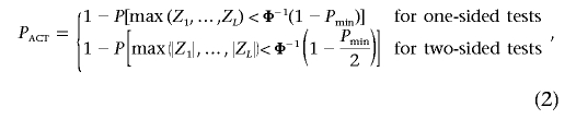with the obvious generalization to a combination of one- and two-sided tests. Figure 1A and 1B illustrates the probabilities for one- and two-sided tests, respectively, when L=2. The elliptical lines represent the contours of the bivariate normal density function. P_ACT is the probability that a random point from this distribution will fall within the shaded area.

Figure 1. .

Bivariate normal probability represented by P_ACT when L=2 for one-sided tests (A) and two-sided tests (B). Elliptical lines represent the contours of a bivariate normal density function with positive correlation. Shaded area represents the space (extending to infinity) over which the probability P_ACT is measured.

If one applies the sequentially rejective multiple-test procedure of Holm,¹³ the ordered P values P_min⩽P₍₂₎⩽P₍₃₎⩽…⩽P_(L) may be adjusted and tested for significance one at a time, starting with P_min. We first adjust P_min for multiple testing by computing P_ACT as in equation (2). If P_ACT<α, the null hypothesis is rejected for the test associated with P_min, and we proceed to P₍₂₎. To adjust P₍₂₎ for multiple testing, we can remove the test associated with P_min from consideration, since the null hypothesis for this test has been rejected. We can now compute P⁽²⁾_ACT according to the formula in equation (2) but replacing P_min with P₍₂₎, L with L-1, and Σ with the covariance matrix between the remaining L-1 tests. If P⁽²⁾_ACT<α, we then reject the null hypothesis associated with P₍₂₎ and compute P⁽³⁾_ACT<α, with P₍₂₎ removed from consideration, continuing in this fashion until P^(k)_ACT⩾α for some k, at which point we conclude that all remaining tests are insignificant. A good example of this kind of sequential testing in the multivariate normal case can be found in the work of Wei et al.⁷

Asymptotic Multivariate Normality of Common Association Test Statistics

Adjustment for multiple correlated tests with P_ACT requires that test statistics be asymptotically distributed as multivariate normal with known covariance matrix. Seaman and Müller-Myhsok¹¹ have shown that, for association tests based on M markers, one can apply the result that a vector of score statistics has a multivariate normal asymptotic distribution under the null hypothesis.¹⁴ We extend this result to include association tests based on correlated traits by deriving the asymptotic distribution for tests of association between M markers and K binary and continuous outcome variables. We show that this result can also be readily applied when multiple genetic models are tested. Although we focus on score tests, these results also apply to Wald and likelihood-ratio tests, since they are asymptotically equivalent to the score test.¹⁵

For each individual (i=1,…,N), let

be a vector of K trait variables (where superscript T indicates transpose), which may include both quantitative traits and binary traits such as disease status. Let G_i be a genotype vector containing allele counts of 0, 1, or 2 for each of M markers, and let X_i be a covariate vector that contains 1 as the first element and that can also include environmental and demographic variables, such as age and sex.

Many of the commonly used tests for association between traits and genotype are based on or related to the score statistics from a generalized linear model. Such tests include the simple test of equal allele frequency for cases and controls, the Cochran-Armitage test for trend,^16,17 and linear and logistic regression. A key assumption of generalized linear models is that

where h is a function, and

where α_k is a vector of covariate effects that includes an intercept term and β_k is an M-dimensional vector of genetic effects. Under this assumption, a linear combination η_ik of genotypes and covariates provides all the information necessary to predict the mean trait value, but the relationship between predicted trait value and η_ik may be nonlinear. For example, in a trend test or logistic regression model,

If K traits are tested for association with M genotypes, the KM-dimensional vector of score statistics is

where is the vector of predicted trait values given covariates, with the assumption of no genetic association, and ⊗ represents the Kronecker product. As we show in appendix A,

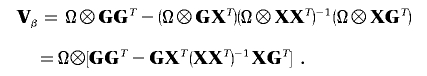
where V_β can be estimated as

the Kronecker product of the sample covariance matrices of traits and genotypes, conditioned on covariates. Here,

and

are matrices of genotypes and covariates, respectively, and

is the trait covariance matrix, conditioned on X.

The P values from individual association tests are generally based on test statistics that are normalized to have variance of 1. A vector of L score statistics, U_β, is easily transformed to a normalized vector of test statistics, T, by computing each element of T as

where U_β,l is the lth element of U_β, and V_β,ll is the lth element along the diagonal of V_β for l=1,…,L; it is also common to work with T²_l=U_β,lV^-1_β,llU_β,l. It is easy to show that , where R is the correlation matrix corresponding to the covariance matrix V_β. With use of this fact, P_ACT can then be computed as in equation (2), given only P_min and R. R, in turn, can generally be estimated as a simple function of the sample correlation matrices of traits and markers, conditioned on any covariates. Appropriate estimates of R are shown for a few examples in table 1.

Table 1. .

Three Examples of Covariance Matrices of Test Statistics R

Example	Trait(s)	Marker(s)	R
1	Two traits with correlation ρ	Single SNP
2	Single trait	Two SNPs with correlation r
3	Two traits with correlation ρ	Two SNPs with correlation r

The above model may be trivially extended to include tests based on multiple genetic models. For example, if a marker is tested for association in three ways, with the assumption of additive, dominant, and recessive models, it can be assigned three elements in G_i, each containing the appropriate genotype code. For instance, the genotype codes for an individual with two copies of the reference allele would be 2, 1, and 1 for the additive, dominant, and recessive models, respectively. The score statistics and covariance matrix are then computed as usual.

Implementation of P_ACT Method

Computation of P_ACT in equation (2) requires integration of the multivariate normal density function. Although the integral has no closed-form solution, multivariate normal probabilities can be integrated numerically when the covariance matrix is known or can be estimated. Genz^18,19 and Genz and Bretz²⁰ have developed a computationally efficient method for numerical integration of the multivariate normal distribution, which is available as Fortran code that can handle integrands of up to 1,000 dimensions.²¹ This Fortran code has been incorporated into the package mvtnorm²² in the R software environment,²³ and the latest version of mvtnorm (versions ⩾0.8) provides sensible estimates of the multivariate normal integral for up to 1,000 dimensions.²² We apply Genz’s algorithm as implemented in mvtnorm to estimate P_ACT for several common association tests. In the interests of computational efficiency, we may choose the requested precision level depending on the magnitude of the P values and the nature of the analysis. For example, one may desire a quick low-precision analysis for exploratory purposes or for clearly nonsignificant results but may want to devote more computational resources to a high-precision final analysis. Our R code for computation of P_ACT is available online (see authors’ Web site).

Assessment of Type I Error Rate and Power

To estimate the type I error rate and power of adjusting for multiple testing with P_ACT, we performed simulations that involved both binary and quantitative traits. In each case, we estimated type I error by simulating 100,000 data sets under the null hypothesis, where trait was assigned at random, independent of genotype. Similarly, we estimated power by creating 10,000 replicate data sets in which trait was influenced by genotype. For each simulation, we performed the relevant set of association tests and computed three overall P values: P_ACT and P_Šidák, as in equations (1) and (2) above, and P_perm. To calculate P_perm, we first created 1,000 permutations of the original data by randomly shuffling individual genotype vectors while leaving the trait data and any covariates intact. In this way, the permuted samples simulated the null hypothesis of no association but maintained the original correlation between genotypes, between traits, and between traits and covariates. We tested each of these 1,000 samples for association and estimated P_perm as the proportion of samples with a minimum P value as low as that observed in the original data. Although 1,000 permutations is much lower than we would use in practice, it is sufficient for estimating type I error and power at the significance level α=.05 that we chose to use.

Binary trait simulations

We simulated case-control status for 1,389 individuals genotyped for 20 HNF1A SNPs as part of the FUSION study of the genetics of type 2 diabetes (T2D).¹² HNF1A is one of six genes known to be involved in maturity-onset diabetes of the young²⁴ and was analyzed by FUSION as a potential candidate gene for T2D.²⁵ Of the 20 SNPs genotyped for the study, most had been chosen to be nonredundant (r²<0.8), and, as figure 2 shows, only moderate LD was present.

Figure 2. .

LD (r²) between 20 SNPs from HNF1A

For type I error estimation, we randomly assigned case-control status in each simulation. For power estimation, we chose 1 of the 20 SNPs as a disease SNP and randomly assigned case-control status according to a multiplicative model of disease risk for each individual, where genotype relative risk (GRR) was chosen to ensure a roughly equal number of cases and controls and a correlation of ∼0.12 between case-control status and the disease gene. This corresponded to a GRR of 1.2 if the disease SNP was our most common SNP, with a minor-allele frequency (MAF) of 0.48, and a GRR of 1.4 if the disease SNP was our least common SNP (MAF=0.04). Individuals missing genotype data for the disease SNP were assigned the mean GRR. To model the common situation in which the genotyped SNPs are proxies for a disease-predisposing variant that was not genotyped, we then omitted the disease SNP from consideration and tested only the remaining 19 SNPs for association when estimating power. For estimation of the type I error rate, there was no disease SNP, so, in this case, we tested all 20 SNPs.

We first tested each of the 19 or 20 SNPs for association with a Cochran-Armitage test for trend,^16,17 which assumes an additive model of disease risk. In each case, we computed P_ACT, P_Šidák, and P_perm to adjust for the 19 or 20 tests. Since 215 individuals were missing data on at least one genotype, we performed each association test by using only individuals with data for the SNP being tested, but we estimated the covariance matrix by using genotype data from all individuals, with missing genotype data for each SNP filled in with the mean allele count for that SNP.

Using the same data, we also tried testing every SNP under the additive, dominant, and recessive models and adjusting for all the tests with P_ACT, P_Šidák, and P_perm. For SNPs with <20 minor-allele homozygotes, we omitted the relevant dominant or recessive model from analysis. This led to the exclusion of four models, for a total of 56 tests, before also removing the disease SNP from consideration.

For the same 1,389 genotyped individuals, we simulated five correlated binary traits according to a probit model. For each simulation, we first generated five equally correlated random variables Z_i1,…,Z_i5 from the multivariate normal distribution for each individual i. For j=1,…,5, each binary trait Y_ij was defined as 1 if Z_ij>0, and 0 otherwise. The resulting five binary traits were equally correlated with one another, with all pairwise correlations ≈0.7. For power estimation, we allowed one trait to be influenced additively by the disease SNP by defining it to be 1 if , and 0 otherwise, where G_i is the disease allele count (0, 1, or 2) for individual i, and is the mean allele count over all individuals with genotypes for the disease SNP. For individuals missing genotypes for the disease SNP, we set to 0. We then used Cochran-Armitage trend tests to test each of the 20 SNPs for association with each of the five traits, for a total of 100 tests (or 95 when the disease SNP is omitted). We again used P_ACT, P_Šidák, and P_perm to adjust for the 95 or 100 tests.

Quantitative-trait simulations

We first simulated data sets of 2,000 individuals with 10 correlated quantitative traits and genotype data for a single SNP with allele frequency 0.5. We assigned trait values according to the linear model Y_ij=α_jX_i+β_jG_i+ɛ_ij, where G_i is the allele count for individual i, X_i is a covariate generated as a linear function of G_i and a random normal component, such that the correlation between X_i and G_i∼0.25, ɛ_ij is a random component, and α_j and β_j are parameters that determine the effect of the covariate and genotype on trait j. For each trait, α_j was drawn from a normal distribution tightly centered around a fixed effect size, so that covariates had a similar, though not identical, effect on the 10 traits. We set β_j=0 for j=1,…,10 when computing type I error and β₁>0 and β_j=0 for j=2,…,10 when computing power. We simulated ɛ_i=(ɛ_i1,ɛ_i2,…,ɛ_i10)^T from the multivariate normal distribution , with one of the five correlation structures shown in figure 3. For each simulation, we tested the SNP for association with each trait separately with a linear regression of the trait value on allele count and the covariate. We used the results from the 10 tests to compute P_Šidák, P_ACT, and P_perm. We performed simulations for lower (0.2), higher (0.7), and extremely high (0.99) values of ρ and τ (where ρ=τ).

Figure 3. .

Correlation structures used in simulations of 10 correlated traits. A, Uncorrelated traits. B, Equal correlation between traits. C, Autocorrelated traits. D, Independent blocks of correlated traits. E, Negatively correlated blocks of correlated traits.

We next randomly drew HNF1A genotypes for each individual and simulated 10 traits, using a similar linear model with no covariates. We tested the traits for association with the 20 HNF1A SNPs, for a total of 200 tests. We estimated type I error as in our previous simulations; to estimate power, we simulated a model where Y_i1 is influenced by the least common of the 20 SNPs (MAF=0.04). When 200 tests were involved, estimation of P_perm was too computationally intensive, so, in this case, we estimated P_Šidák and P_ACT only.

Finally, we performed both the single-SNP and 20-SNP simulations for a set of five binary and five continuous traits. We generated 10 multivariate normal random variables according to the model Z_ij=α_jX_i+β_jG_i+ɛ_ij, with X_i, G_i, ɛ_ij, α_j, and β_j defined as above. We defined the five continuous traits as Y_ij=Z_ij for j=1,…,5 and the five binary traits by setting Y_ij=1 if Z_ij>1.25, and 0 otherwise, for j=6,…,10. Each binary trait had a prevalence of ∼0.1, and we chose the covariance of ɛ_i, such that all pairwise trait correlations were between 0.5 and 0.7. We estimated type I error and power as in previous simulations.

Performance of other methods

We also used the simulations described above to estimate the type I error rate for two methods that estimate an effective number of tests (see introductory paragraphs). For the method of Cheverud² and Nyholt,³ we computed the effective number of tests as , where L is the number of tests performed and is the variance of the eigenvalues from the correlation matrix between the tests. For the method of Li and Ji,⁴ we computed the effective number of tests as

where is 1 if the absolute value of the ith eigenvalue , and 0 otherwise, and is the largest integer ⩽. For each method, we computed a multiple-testing–adjusted P value by substituting the effective number of tests for L in the Šidák formula. We then estimated the type I error rate as described above.

Comparison Between P_ACT and P_perm in FUSION Data

To assess how closely estimates of P_ACT correspond to gold-standard estimates based on P_perm, we analyzed 3,575 SNPs in and near 224 candidate genes that were genotyped for 1,161 T2D-affected subjects and 1,174 control individuals with normal glucose tolerance from the FUSION study (K. L. Mohlke, personal communication). We first tested the 3,007 SNPs that had ⩾20 individuals in each of the three genotype classes for association with T2D, using the additive, dominant, and recessive models and controlling for age category, sex, and birth region as covariates. For each SNP, we estimated both P_ACT and P_perm to adjust for the three tests, providing 3,007 comparisons between P_ACT and P_perm.

We next tested all 3,575 SNPs for association with 18 quantitative T2D-related traits (residualized on age category, sex, and birth region) on the 1,174 controls. For each SNP, we estimated both P_ACT and P_perm, to adjust for the 18 correlated tests, which provided 3,575 comparisons between P_ACT and P_perm. To provide additional comparisons between P_ACT and P_perm for highly significant tests, we simulated nine additional SNPs with minimum P values of 1×10^-5, 5×10^-6, 2.5×10^-6, 1×10^-6, 5×10^-7, 2.5×10^-7, 1×10^-7, 5×10^-8, and 2.5×10^-8 and adjusted these minimum P values for multiple testing with P_ACT and P_perm.

For all comparisons, we computed P_ACT at increased precision for more-significant SNPs and under the assumption that covariates were independent of genotype. For P_perm, we performed 1,000,000 permutations for the 10 most-significant SNPs, 100,000 for the next 190 significant SNPs, and 10,000 for all other SNPs. For the nine SNPs simulated to be highly significant, we performed 10,000,000 permutations.

Results

Type I Error Rate and Power for Simulated Data

Table 2 presents estimates of type I error rate (first row) and power (subsequent rows) for P_Šidák, P_ACT, and P_perm when the 20 HNF1A SNPs are tested for disease association. The estimates in the first row (based on 100,000 simulation replicates each) show that both P_ACT and P_perm have type I error rates ∼0.05 and are thus valid in all cases considered—that is, when the 20 SNPs are tested for association with a binary trait under an additive model or under three competing models or when the SNPs are tested for association with five correlated binary traits. Tests based on P_Šidák are conservative in each case. A similar pattern was observed for α levels of .01, .001, and .0001 or when the true model was dominant or recessive (data not shown).

Table 2. .

Type I Error Rate and Power When 20 HNF1A SNPs Are Tested for Association with Binary Traits

				One Binary Trait Tested						Five Binary Traits Tested
				On Additive Model			On Three Models			On Additive Model
Disease SNP	MAF	r2totala	r2maxb	PŠidák	PACT	Pperm	PŠidák	PACT	Pperm	PŠidák	PACT	Pperm
None (type I error)	…	…	…	.0301	.0503	.0507	.0247	.0500	.0508	.0259	.0495	.0502
Most common SNP	.48	.88	.78	.899	.927	.925	.859	.911	.910	.806	.857	.859
Moderately frequent SNP	.20	.93	.19	.419	.535	.538	.338	.482	.484	.280	.385	.377
Least common SNP	.04	.91	.79	.878	.916	.915	.811	.874	.874	.686	.772	.773
SNP least predicted by others	.05	.42	.35	.387	.475	.476	.296	.401	.402	.220	.304	.299

^ar²_total = Proportion of variance in disease SNP allele count explained by the other 19 SNPs.

^br²_max = Maximum pairwise r² between disease SNP and each of the other 19 SNPs.

Each of the next four rows of table 2 present power estimates with a different SNP modeled as the disease-predisposing SNP: the most common SNP (MAF=0.48), a moderately frequent SNP (MAF=0.20), the least common SNP (MAF=0.04), and the SNP least well predicted by a linear function of the others. The power estimates (based on 10,000 simulation replicates each) show that tests based on P_ACT have near identical power to permutation tests and are consistently more powerful than tests performed with Šidák (or Bonferroni) adjustment. Results were similar for the other 16 SNPs (data not shown).

Table 3 presents estimates of type I error rate and power for tests of association with traits correlated as in figure 3, with ρ=τ=0.7; data are presented for 10 quantitative traits in rows 1–5 and for five binary and five quantitative traits in row 6. When a single SNP is tested for association, P_ACT and P_perm provide valid tests and P_Šidák is overly conservative, except when traits are independent, as in the first row of table 3. There is near identical power for P_ACT and P_perm, whereas P_Šidák has reduced power in each situation except independence. Results are similar even when 20 correlated SNPs are tested for association with 10 correlated traits, for a total of 200 tests. Similar results were also observed for lower levels of correlation (ρ=τ=0.2) (data not shown) and extremely high levels of correlation (ρ=τ=0.99) (data not shown). As expected, the power gains of P_ACT and P_perm over P_Šidák were smaller when ρ=τ=0.2 and were greater when ρ=τ=0.99.

Table 3. .

Type I Error Rate and Power When 10 Correlated Quantitative Traits Are Tested for Association

	10 Traits Tested for Association with
	One SNP and a Covariate						20 Correlated HNF1A SNPs
	Type I Error Rate			Power			Type I Error Rate		Power
Trait Correlation Structure	PŠidák	PACT	Pperm	PŠidák	PACT	Pperm	PŠidák	PACT	PŠidák	PACT
Independent traits	.0498	.0499	.0496	.819	.819	.816	.0325	.0514	.780	.821
Equicorrelated traits	.0302	.0502	.0503	.826	.880	.878	.0216	.0507	.778	.852
Autocorrelated traits	.0393	.0494	.0495	.820	.842	.839	.0274	.0499	.777	.833
Independent blocks of traits	.0386	.0497	.0501	.824	.850	.848	.0264	.0501	.779	.836
Negatively correlated blocks of traits	.0327	.0496	.0500	.825	.870	.868	.0234	.0503	.779	.846
Five binary and five quantitative traits	.0341	.0491	.0488	.825	.864	.860	.0263	.0517	.781	.844

We ran additional simulations testing up to 1,000 equicorrelated quantitative traits (ρ=0.7) for association with a single SNP and a covariate (data not shown). For 300, 400, and 500 tests, respective estimated type I error rates were .0121, .0112, and .0102 for P_Šidák and were .0506, .0499, and .0517 for P_ACT, which suggests that P_ACT can achieve the target type I error rate for several hundred tests, whereas P_Šidák is increasingly conservative. For 600, 750, and 1,000 tests, the respective estimated type I error rates were .0102, .0093, and .0086 for P_Šidák and were .0550, .0593, and .0648 for P_ACT, which indicates a possible bias or reduction in the precision of P_ACT when the number of tests is extremely large.

For the two methods based on the effective number of tests (data not shown), we found that the methods of Cheverud² and Nyholt³ tended to be overly conservative and that the method of Li and Ji⁴ was anticonservative in all cases, except when tests were completely independent. When a binary trait was tested for association with 20 HNF1A SNPs, the type I error rates for the two methods were 0.0389 and 0.0613 for just the additive model and were 0.0297 and 0.0667 when three genetic models were tested. When 10 traits were tested for association with a single SNP and a covariate, both methods had a type I error rate ∼0.05 when traits were independent; for the other trait-correlation structures, the type I error rate had a range of 0.0460–0.0504 with the Cheverud and Nyholt methods and of 0.0615–0.0666 with the method of Li and Ji.⁴

P_ACT and P_perm in FUSION Data

Figure 4 shows the relationship between P_ACT and P_perm in the context of a FUSION study of 3,575 SNPs in 224 candidate genes for T2D (K. L. Mohlke, personal communication). P_ACT and P_perm are plotted on a log scale to emphasize the smallest P values (upper right of the fig. 4 panels). We obtained the values of P_ACT and P_perm in figure 4A by testing each SNP for association under the additive, dominant, and recessive models and by adjusting the minimum P value from these three tests for multiple testing. We obtained the values of P_ACT and P_perm in figure 4B by testing each SNP for association with 18 correlated T2D-related traits and adjusting the minimum P value for each SNP for the 18 tests. Figure 4B also includes data for nine highly significant simulated SNPs, indicated by blackened circles. In all cases, P_ACT and P_perm track each other quite closely, with all points falling very near the identity line (r²>0.999 for both figures).

Figure 4. .

A, Estimates of P_ACT and P_perm for 3,007 SNPs tested for disease association under three genetic models. B, Estimates of P_ACT and P_perm for 3,584 SNPs tested for association with 18 quantitative traits. Unblackened circles represent 3,575 SNPs genotyped for the candidate-gene study. Blackened circles represent nine simulated SNPs.

Computation Speed: Comparisons of Methods

Because the goal of our proposed method is to estimate P values with the same accuracy and precision as permutation tests in less time, we timed computation of P values at a constant level of precision. We compared timings for P_ACT, P_perm, and one of the simulation-based methods (described above) that has been shown to attain the accuracy of permutation tests—the direct simulation approach (DSA) of Seaman and Müller-Myhsok.¹¹ We implemented all three methods in R, using the code for the DSA provided on the authors’ Web site. For each method, we measured the time required to compute an adjusted P value for a fixed P_min (chosen such that p_ACT, P_DSA, or P_perm≈.0001) at a given level of precision (SE⩽0.00001). Attainment of this level of precision requires ∼1,000,000 permutations for P_perm and ∼1,000,000 simulations for P_DSA. Since the speed of P_perm depends on sample size, we present timings for three typical sample sizes. For computational efficiency, we tested for association with a simple Cochran-Armitage test for trend^16,17; models requiring additional computation, such as logistic or even linear regression, would have penalized the permutation tests to a much greater degree. For example, if we had instead tested for association with a logistic-regression model of trait on genotype with age and sex as covariates, the timings for P_ACT and P_DSA would show no noticeable change, but computation of P_perm would have taken >300 times longer.

Table 4 compares timings for P_ACT, P_perm, and P_DSA for three representative situations. The first row shows timings when 200 autocorrelated tests are adjusted for multiple testing. This example is meant to approximate the correlation between a series of nonredundant SNPs along a chromosome, since correlation is generally high between neighboring SNPs and decays with distance. In this case, computing P_ACT is ∼60 times faster than computing P_DSA and thousands of times faster than computing P_perm. Similar timings for 20, 40, 60, 80, and 100 autocorrelated tests demonstrate that the computational time required increases approximately linearly to the number of tests for all three estimators (data not shown). We also computed P_ACT for even smaller P values and greater dimension. Adjustment of a minimum P value of 10⁻⁸ with P_ACT with SE⩽10% of the estimate required 11 s for 200 autocorrelated tests, 25 s for 500 tests, and 70 s for 1,000 tests. The same computation for only 200 tests would have required >3 h for P_DSA and 100–800 h for P_perm, depending on sample size.

Table 4. .

Computation Time Required to Estimate a P Value of .0001 with SE ⩽.00001

	Computation Time
	PACT	PDSA	Pperm
Correlation Structure	Any N	Any N	N=200	N=1,000	N=2,000
200 Autocorrelated SNPs	3.54 s	212 s	1.75 h	10.8 h	13.9 h
HNF1A with 20 SNPs	.71 s	43.8 s	825 s	2,044 s	1 h
20,000 HNF1As with 20 SNPs each	3.94 h	10.1 d	.52 years	1.29 years	2.28 years

The second row of table 4 presents the computational time required to test the 20 HNF1A SNPs for association. In this case, P_ACT can be computed 60 times faster than P_DSA and up to 5,000 times faster than P_perm. The third row uses the information from the second to consider the prospect of 20,000 independent blocks of 20 SNPs with the correlation structure of HNF1A, illustrating what might occur if we tested sets of SNPs from every gene in the human genome. In this situation, permutation testing is essentially infeasible except with massive amounts of parallelization, whereas the same analysis can be performed with P_ACT in a single afternoon.

Discussion

Permutation testing, when performed appropriately, provides an unbiased test of the null hypothesis and is widely considered the gold standard with which other estimators and tests can be compared. Its main disadvantages are the time and computational resources required to obtain precise P value estimates, so alternative tests that provide similar results with less computational burden can be quite attractive, particularly when a large number of tests is involved or when data are frequently reanalyzed in light of new samples or genotypes.

Whereas conventional distribution-based statistical tests typically require minimal computational resources, permutation tests are often employed when the asymptotic distribution of the statistic is unknown or difficult to model. However, for many of the tests commonly used in GWA studies, the asymptotic joint distribution of the test statistics is known, which makes analytical methods possible. As we show above, the asymptotic distribution of test statistics from association tests between correlated traits, markers, and models is often multivariate normal with known covariance matrix. However, the most significant test statistic from a group of multivariate normal test statistics has a distribution function that, although known, cannot be computed analytically because of the lack of a closed-form solution to the multivariate normal integral. Lin¹⁰ and Seaman and Müller-Myhsok¹¹ have suggested simulation-based approaches that can approximate the null distribution of ordered test statistics much more quickly than can permutation tests. Our P_ACT method relies on numerical integration of the distribution function and can approximate the null distribution much more quickly than permutation or simulation-based approaches.

The data presented here suggest that tests based on P_ACT are appropriate substitutes for those based on permutation testing, since P_ACT consistently attains results essentially identical to those of permutation-based P values, both for simulated data and over thousands of association tests performed as a part of a large candidate-gene study (K. L. Mohlke, personal communication). Whereas Lin¹⁰ and Seaman and Müller-Myhsok¹¹ have also demonstrated that their estimators (denoted here as P_Lin and P_DSA, respectively) provide valid tests and attain the accuracy of P_perm, P_ACT demonstrates greater gains in computational efficiency. P_ACT is typically thousands of times faster than permutation-based P values at a given level of precision. This makes P_ACT potentially useful in the contexts of both large-scale candidate-gene studies, in which thousands of tests may be performed, and GWA studies, in which millions of tests may be performed. Since the precision of this method can be traded for speed, P_ACT can be tailored both to initial exploratory tests for which speed is especially important and to more-definitive tests for which greater precision is needed; it can also be computed at increased precision for more-interesting results.

Like any estimator, P_ACT is not appropriate for every analysis. It was designed to adjust the minimum P value and other ordered P values for a large number of 1-df tests. An advantage of this method is that it allows easy identification of the particular traits, variants, and genetic models associated with the most-interesting results. This approach is especially relevant if we are looking for a small number of reasonably large genetic effects. If we instead expect a large number of very small effects, a joint analysis of all associations simultaneously might be more appropriate. Typically, these methods are based on multiple-df tests, which are outside the scope of P_ACT, but P_Lin and P_DSA remain useful alternatives to permutation testing in those situations. For example, the DSA software computes an adjusted P value for product methods,^26,27 as well as for the minimum P value.¹¹

The validity of P_ACT (as well as that of P_Lin and P_DSA) depends on knowledge of the correct asymptotic distribution. Although many common association test statistics are asymptotically multivariate normal, use of the asymptotic distribution requires reasonably large sample sizes and cell counts and may not be appropriate in all cases—for example, dominant or recessive models with a rare minor allele. The solution we have employed here and elsewhere (K. L. Mohlke, personal communication)^25,28 is to drop dominant or recessive models with low cell counts from the analysis; another solution would be to rely on exact tests, such as Fisher’s exact test, for these models. A related issue is that sample size must be substantially larger than the number of tests for asymptotic properties to hold; however, simulations have shown that P_Lin can achieve the target type I error rate when the number of tests far exceeds the sample size.¹⁰ For situations where the asymptotic distribution is unknown or the sample size is too small for asymptotic properties to hold, however, permutation testing may be the appropriate choice. The algorithm of Kimmel and Shamir,²⁹ which relies on importance sampling to sample from the null distribution in a way that mimics permutation testing, can also be computed thousands of times faster than permutation tests and does not require assumptions about the asymptotic distribution. A direct comparison of the asymptotic methods discussed here and this importance sampling method has not been performed but would be of great interest.

The validity of P_ACT and P_DSA also depends on accurate estimation of the covariance matrix. Improper handling of missing trait or genotype data can lead to biased covariance estimates. Although it is rare for samples to contain complete genotype and trait data for every individual, only individuals with complete data can be used in computation of sample covariance matrices; otherwise, the matrices may not be positive definite. However, exclusion of individuals with incomplete data may lead to biased estimates of the covariance matrix. Seaman and Müller-Myhsok¹¹ suggest performing the entire analysis with missing genotype data imputed, but Lin³⁰ argues that imputation can adversely impact type I error. Lin’s estimator is based on individual contributions to the score statistic, and he treats missing data for an individual by setting the individual component of the appropriate score statistic(s) to 0. In the case of P_ACT, an analogous approach is to test each trait and marker only on individuals with complete data for that trait and marker but to estimate the covariance matrix of the tests for the full sample, with missing data for marker m (or trait k) filled in with the mean genotype score for marker m (or the mean value for trait k), conditional on covariates. Although >15% of individuals in our first set of simulations (table 2) were missing data on at least one genotype, P_ACT achieved the target type I error when this approach was used.

Valid covariance-matrix estimation also depends on how many tests are considered at once. The numerical integration method implemented in the package mvtnorm²² has proved reliable in testing of 750-dimensional integrals (A. Genz, personal communication), and we observed that high levels of precision are possible for up to 1,000 dimensions. However, even with reliable numerical integration, precision of the covariance estimates may suffer as the ratio between the number of parameters in the covariance matrix and the number of usable samples increases. In our simulations, tests based on P_ACT with samples of 2,000 were consistently valid for 200 dimensions and appeared to be valid in examples with 300–500 tests. However, in the examples we considered with 600–1,000 tests, P_ACT did not achieve the target type I error rate. Further investigation of the appropriate upper limits on dimension and how they relate to sample size is warranted. Seaman and Müller-Myhsok¹¹ treat 0.1 as the upper limit for the ratio of number of tests (L) to sample size (N), which seems an appropriate rule of thumb, since the eigenvalues of a sample covariance matrix resemble the eigenvalues of the true matrix quite closely when L⩽N/10.³¹ Given conventional sample sizes, large-scale candidate-gene studies are quite feasible within such a limit, and we have already used P_ACT in several (K. L. Mohlke, personal communication).^25,28

With GWA studies becoming a priority, there is also potential for P_ACT to be useful on a larger scale. One possible strategy is to break up large analyses into roughly independent blocks of hundreds of tests each.¹¹ If we then compute P_ACT for each group of tests, the Šidák procedure can be used to adjust the most-significant values of P_ACT for the number of blocks via the sequential Holm¹³ procedure (see the “Methods” section). As long as the correlation between the blocks of tests is reasonably low, little power will be sacrificed by approximating in this way, since P_ACT has accounted for the correlation within the blocks. Use of the P_ACT method in such a framework has the potential to facilitate exploration of the genome by highlighting our most-significant findings without imposing an overly severe penalty when hundreds, thousands, or millions of association tests are performed.

Appendix A

Written in terms of covariate effects, the KM-dimensional vector of score statistics is

where is the vector

and is the maximum-likelihood estimate of α_k when β_k is restricted to 0. A first-order Taylor expansion gives us

where and α are the stacked vectors

and

respectively. The multivariate central limit theorem³² may be applied to show that

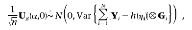where η_i is the vector

Since, under the null hypothesis, and G are independent with mean 0,

can be estimated efficiently by Ω⊗GG^T, where

It is also easily shown through Taylor expansion of that

where

can be estimated by Ω^-1⊗XX^T. Finally,

which has sample analogue Ω⊗GX^T. Hence,

where

References

- 1.Šidák Z (1967) Rectangular confidence regions for the means of multivariate normal distributions. J Am Stat Assoc 62:626–633 10.2307/2283989 [DOI] [Google Scholar]
- 2.Cheverud JM (2001) A simple correction for multiple comparisons in interval mapping genome scans. Heredity 87:52–58 10.1046/j.1365-2540.2001.00901.x [DOI] [PubMed] [Google Scholar]
- 3.Nyholt DR (2004) A simple correction for multiple testing for single-nucleotide polymorphisms in linkage disequilibrium with each other. Am J Hum Genet 74:765–769 [DOI] [PMC free article] [PubMed] [Google Scholar]
- 4.Li J, Ji L (2005) Adjusting multiple testing in multilocus analysis using the eigenvalues of a correlation matrix. Heredity 95:221–227 10.1038/sj.hdy.6800717 [DOI] [PubMed] [Google Scholar]
- 5.Dudbridge F, Koeleman BP (2004) Efficient computation of significance levels for multiple associations in large studies of correlated data, including genomewide association studies. Am J Hum Genet 75:424–435 [DOI] [PMC free article] [PubMed] [Google Scholar]
- 6.Salyakina D, Seaman SR, Browning BL, Dudbridge F, Müller-Myhsok B (2005) Evaluation of Nyholt’s procedure for multiple testing correction. Hum Hered 60:19–25 10.1159/000087540 [DOI] [PubMed] [Google Scholar]
- 7.Wei LJ, Lin DY, Weissfeld L (1989) Regression analysis of multivariate incomplete failure time data by modeling marginal distributions. J Am Stat Assoc 84:1065–1073 10.2307/2290084 [DOI] [Google Scholar]
- 8.Wei LJ, Glidden DV (1997) An overview of statistical methods for multiple failure time data in clinical trials. Stat Med 16:833–839 [DOI] [PubMed] [Google Scholar]
- 9.James S (1991) Approximate multinormal probabilities applied to correlated multiple endpoints in clinical trials. Stat Med 10:1123–1135 10.1002/sim.4780100712 [DOI] [PubMed] [Google Scholar]
- 10.Lin DY (2005) An efficient Monte Carlo approach to assessing statistical significance in genomic studies. Bioinformatics 21:781–787 10.1093/bioinformatics/bti053 [DOI] [PubMed] [Google Scholar]
- 11.Seaman SR, Müller-Myhsok B (2005) Rapid simulation of P values for product methods and multiple-testing adjustment in association studies. Am J Hum Genet 76:399–408 [DOI] [PMC free article] [PubMed] [Google Scholar]
- 12.Valle T, Tuomilehto J, Bergman RN, Ghosh S, Hauser ER, Eriksson J, Nylund SJ, Kohtamaki K, Toivanen L, Vidgren G, et al (1998) Mapping genes for NIDDM: design of the Finland–United States Investigation of NIDDM Genetics (FUSION) study. Diabetes Care 21:949–958 10.2337/diacare.21.6.949 [DOI] [PubMed] [Google Scholar]
- 13.Holm S (1979) A simple sequentially rejective multiple test procedure. Scand J Stat 6:65–70 [Google Scholar]
- 14.McCullagh P, Nelder JA (1989) Generalized linear models, 2nd ed. Chapman and Hall, London [Google Scholar]
- 15.Cox DR, Hinkley DV (1974) Theoretical statistics. Chapman and Hall, London [Google Scholar]
- 16.Cochran WG (1954) Some methods for strengthening the common χ2 tests. Biometrics 10:417–451 10.2307/3001616 [DOI] [Google Scholar]
- 17.Armitage P (1955) Tests for linear trends in proportions and frequencies. Biometrics 11:375–386 10.2307/3001775 [DOI] [Google Scholar]
- 18.Genz A (1992) Numerical computation of multivariate normal probabilities. J Comput Graph Stat 1:141–149 10.2307/1390838 [DOI] [Google Scholar]
- 19.Genz A (1993) Comparison of methods for the computation of multivariate normal probabilities. Comput Sci Stat 25:400–405 [Google Scholar]
- 20.Genz A, Bretz F (2002) Comparison of methods for the computation of multivariate t-probabilities. J Comput Graph Stat 11:950–971 10.1198/106186002321018885 [DOI] [Google Scholar]
- 21.Genz A (2000) MVTDST: a set of Fortran subroutines, with sample driver program, for the numerical computation of multivariate t integrals, with maximum dimension 100 (increased to 1000—7/07) (available at http://www.math.wsu.edu/faculty/genz/homepage) (accessed October 15, 2007)
- 22.Genz A, Bretz F, Hothorn T (2007) mvtnorm: multivariate normal and t distribution. R package version 0.8–0 (available at http://cran.r-project.org/doc/packages/mvtnorm.pdf) (accessed October 25, 2007)
- 23.R Development Core Team (2007) R: a language and environment for statistical computing. R Foundation for Statistical Computing, Vienna (available at http://www.r-project.org/) (accessed October 25, 2007)
- 24.Fajans SS, Bell GI, Polonsky KS (2001) Molecular mechanisms and clinical pathophysiology of maturity-onset diabetes of the young. N Engl J Med 345:971–980 10.1056/NEJMra002168 [DOI] [PubMed] [Google Scholar]
- 25.Bonnycastle LL, Willer CJ, Conneely KN, Jackson AU, Burrill CP, Watanabe RM, Chines PS, Narisu N, Scott LJ, Enloe ST, et al (2006) Common variants in maturity-onset diabetes of the young genes contribute to risk of type 2 diabetes in Finns. Diabetes 55:2534–2540 10.2337/db06-0178 [DOI] [PubMed] [Google Scholar]
- 26.Fisher RA (1932) Statistical methods for research workers. Oliver and Boyd, London [Google Scholar]
- 27.Zaykin DV, Zhivotovskty LA, Westfall PH, Weir BS (2002) Truncated product method for combining p-values. Genet Epidemiol 22:170–185 10.1002/gepi.0042 [DOI] [PubMed] [Google Scholar]
- 28.Willer CJ, Bonnycastle LL, Conneely KN, Duren WL, Jackson AU, Scott LJ, Narisu N, Chines PS, Skol A, Stringham HM, et al (2007) Screening of 134 single nucleotide polymorphisms (SNPs) previously associated with type 2 diabetes replicates association with 12 SNPs in nine genes. Diabetes 56:256–264 10.2337/db06-0461 [DOI] [PubMed] [Google Scholar]
- 29.Kimmel G, Shamir R (2006) A fast method for computing high-significance disease association in large population-based studies. Am J Hum Gen 79:481–492 10.1086/507317 [DOI] [PMC free article] [PubMed] [Google Scholar]
- 30.Lin DY (2005) On rapid simulation of P values in association studies. Am J Hum Genet 77:513–514 [DOI] [PMC free article] [PubMed] [Google Scholar]
- 31.Schäfer J, Strimmer K (2005) A shrinkage approach to large-scale covariance-matrix estimation and implications for functional genomics. Stat Appl Genet Mol Biol 4:article 32 [DOI] [PubMed] [Google Scholar]
- 32.Cramér H (1946) Mathematical methods of statistics. Princeton University Press, Princeton, NJ [Google Scholar]