Symmetric Diffeomorphic Image Registration with Cross-Correlation: Evaluating Automated Labeling of Elderly and Neurodegenerative Brain

Abstract

One of the most challenging problems in modern neuroimaging is detailed characterization of neurodegeneration. Quantifying spatial and longitudinal atrophy patterns is an important component of this process. These spatiotemporal signals will aid in discriminating between related diseases, such as frontotemporal dementia (FTD) and Alzheimer’s disease (AD), which manifest themselves in the same at-risk population. Here, we develop a novel symmetric image normalization method (SyN) for maximizing the cross-correlation within the space of diffeomorphic maps and provide the Euler-Lagrange equations necessary for this optimization. We then turn to a careful evaluation of our method. Our evaluation uses gold standard, human cortical segmentation to contrast SyN’s performance with a related elastic method and with the standard ITK implementation of Thirion’s Demons algorithm. The new method compares favorably with both approaches, in particular when the distance between the template brain and the target brain is large. We then report the correlation of volumes gained by algorithmic cortical labelings of FTD and control subjects with those gained by the manual rater. This comparison shows that, of the three methods tested, SyN’s volume measurements are the most strongly correlated with volume measurements gained by expert labeling. This study indicates that SyN, with cross-correlation, is a reliable method for normalizing and making anatomical measurements in volumetric MRI of patients and at-risk elderly individuals.

1 Introduction

Frontotemporal dementia (FTD) prevalence may be higher than previously thought and may rival Alzheimer’s disease (AD) in individuals younger than 65 years [1]. Because FTD can be challenging to detect clinically, it is important to identify an objective method to support a clinical diagnosis. MRI studies of individual patients are difficult to interpret because of the wide range of acceptable, age-related atrophy in an older cohort susceptible to dementia. This has prompted MRI studies that look at both the rate and the anatomic distribution of change [2–7].

Manual, expert delineation of image structures enables in vivo quantification of focal disease effects and serves as the basis for important studies of neurodegeneration [4]. Expert structural measurements from images also provide the gold-standard of anatomical evaluation. The manual approach remains, however, severely limited by the complexity of labeling 256³ or more voxels. Such labor is both time consuming and expensive to support, while the number of individual experts available for such tasks is limited. A third significant difficulty is the problem of inter-rater variability which limits the reliability of manual labeling [8]. While rarely available for large-scale data processing, an expert eye remains valuable for limited labeling tasks that give a basis for algorithmic evaluation.

Deformable image registration algorithms are capable of functioning effectively in time-sensitive clinical applications [9] and high-throughput environments and are used successfully for automated labeling and measurement research tasks. One challenge is reliable performance on non-standard data, as in studies of potentially severe neurodegenerative disorders. These types of images violate the basic assumptions of small deformations and/or simple intensity relationships used in many existing image registration methods.

Diffeomorphic image registration algorithms hold the promise of being able to deal successfully with both small [10–16] and large deformation problems [17–26]. State of the art methods also give full space-time optimizations, are symmetric with respect to image inputs and allow probabilistic similarity measures [27]. Inverse consistent image registration (ICIR) is an additional common alternative to diffeomorphic mapping. Inverse consistency was first introduced by Thirion as an extension to his Demons algorithm [28] but was popularized by Johnson and Christensen [29] and others [30]. Symmetric methods are distinct from ICIR in that symmetric algorithms, first, guarantee that results are identical regardless of the order of input data and, second, use exact inverse transformations guaranteed by diffeomorphisms. Inverse consistency approximates symmetry by including variational penalties in the normalization optimization algorithm. Depending on the weights of the various data, regularization and inverse consistency terms, consistency may be satisfied (or not) at the expense of the other matching criterion. Furthermore, inverse consistent algorithms use approximate inverse transformations [29]. Because the inverse transformations themselves are approximate, the consistency term, as well, is compromised.

Here, we develop a novel symmetric diffeomorphic optimizer for maximizing the cross-correlation in the space of topology preserving maps. The cross-correlation measure has been used in medical image registration before [10,11,31] and more extensively in computer vision. However, this measure has not been investigated for the diffeomorphic case. Furthermore, it has not been used in symmetric normalization or “inverse consistent” studies. Applying our novel normalization formulation to cross-correlation provides the advantage (or option) of symmetrizing the cross-correlation Euler-Lagrange equations. We show that these symmetric Euler-Lagrange equations can be computed with only minor additional computational costs. We then give a careful evaluation of the performance of our symmetric diffeomorphic algorithm for high dimensional normalization of elderly and neurodegenerative cortical anatomy. We compare the method to an elastic cross-correlation optimizer as well as the Demons algorithm which was shown to outperform other methods in a careful evaluation of inter-subject brain registration [32].

2 Registration Methods

2.1 Demons

Thirion’s Demons algorithm [33] is known to perform well in inter-subject deformable image registration. The method uses an approximate elastic regularizer to solve an optical flow problem, where the “moving” image’s level sets are brought into correspondence with those of a reference or “fixed” template image. In practice, the algorithm computes an optical flow term which is added to the total displacement (initially zero). The total displacement is then smoothed with a Gaussian filter. The process repeats for a set number of iterations for each resolution in a multi-resolution optimization scheme. The method is freely available in the Insight ToolKit and has been optimized by the ITK community (www.itk.org).

Dawant et al. used the Demons algorithm for segmenting the caudate nucleus, the brain and the cerebellum for a morphometric comparison of normal and chronic alcoholic individuals [34]. Their evaluation of the algorithm found reasonable agreement between automated and manual labeling. They also showed results on the automated labeling of hippocampus but did not evaluate performance. Their comparison used the Dice statistic (overlap ratio),

$$S(R1,R2)=\frac{2\#(R1\cap R2)}{\#(R1)+\#(R2)},$$ (1)

which measures both difference in size and location between two segmentations, R1 and R2. The #(R) operator counts the number of pixels in the region, R. This sensitive measure varies in the range [0, 1] where values greater than 0.6 for smaller structures and 0.8 for larger structures are considered good by some authors [34,8].

The range of acceptable values for the Dice statistic are, of course, highly dependent upon the application. Both the amount of certainty that one has in the “gold standard” dataset and, also, the specific use of the segmentations determine a reasonable operating range. Our goal, in this paper, is to use manually segmented structures as a foundation for comparing automated normalization methods. In this respect, it is relative performance (measured with respect to the Dice statistic) that is of critical value.

2.2 Symmetric Diffeomorphisms

A diffeomorphism is a differentiable map with a differentiable inverse [35,36]. We typically restrict our solutions to the diffeomorphic space Diff₀ with homogeneous boundary conditions. That is, we assume that rigid and scaling transformations have been factored out and the image border maps to itself¹. Shortest paths between elements in this space are termed geodesic. Diffeomorphic methods were introduced into medical computer vision [17] for the purpose of providing a group theoretical, large deformation space-time image registration framework. Current developments in large deformation computational anatomy by Miller, Trouve and Younes extended the methods to include photometric variation and to use Euler-Lagrange equations [22]. However, the standard version of these methods, Beg’s Large Deformation Diffeomorphic Metric Matching (LDDMM) [23], do not formulate the transformation optimization symmetrically. They are only symmetric in theory and their implementation requires parallel computation. Through personal communication, however, we understand that a symmetrization operator, based on the transformation Jacobian, is being included in current developments by Younes and Trouv’e [37,38]. However, these methods do not guarantee symmetry for similarity metrics other than the intensity difference.

Our current work extends the Lagrangian diffeomorphic registration technique described in [39]. This new formulation has symmetry properties required for a geodesic connecting two images, I and J, in the space of diffeomorphic transformations and guarantees symmetry regardless of the chosen similarity measure. This formulation accounts for the natural symmetry in the problem: both images move along the shape (diffeomorphism) manifold. Symmetric diffeomorphisms guarantee two properties that are intrinsic to the notion of a geodesic path: the path from I to J is the same as it is when computed from J to I, regardless of similarity metric or optimization parameters. Symmetry is required for distance estimates and makes results independent of arbitrary decisions about which image is “fixed” or “moving.”

Our method is also unique in that it guarantees sub-pixel accurate, invertible transformations in the discrete domain by directly including invertibility constraints in the optimization. While diffeomorphisms are theoretically guaranteed to be invertible, interpolation errors can lead to invertibility errors that increase linearly with the number of interpolation steps. Our solution, on the other hand, directly minimizes this error by exploiting the invertibility guaranteed by diffeomorphisms. Finally, the method is efficient enough to use on single-processor machines and in processing large datasets.

We define a diffeomorphism φ of domain Ω, generally, for transforming image I into a new coordinate system by φI = I ○ φ(x, t = 1). The parameters of these transformations are time, t, a spatial coordinate, x, and a velocity field, υ(x, t) on Ω, which is a square-integrable, continuous vector field [36]. The correspondence maps, φ, are gained by integrating the velocity fields in time, $\phi (\mathbf{x},1)=\phi (\mathbf{x},0)+{\int }_0^1\mathit{\upsilon }(\phi (\mathbf{x},t),t)dt$; the distance is then $D(\phi (\mathbf{x},0),\phi (\mathbf{x},1))={\int }_0^1\left|\right|\mathit{\upsilon }(\mathbf{x},t)|{|}_{L}dt$, where L defines the linear operator regularizing the velocity. The functional norm, || · ||_L, induces regularity on the velocity field via a linear differential operator such as L = a∇² + bId (a, b constants). Such a diffeomorphism gives a dense map in both space and time and is illustrated in figure 1. A basic fact of diffeomorphisms allows them to be decomposed into two parts, φ₁ and φ₂. We exploit this fact to define a variational energy that explicitly divides the image registration diffeomorphisms into two halves such that I and J contribute equally to the path and deformation is divided between them. Assume that x indicates the identity position of some anatomy in image I and z indexes the identity position of the same anatomy in image J. We assume, also, that the diffeomorphism maps homologous anatomy in these images. The prior knowledge that this diffeomorphic map should apply evenly to both images can be captured by including the constraint D(Id, φ₁(x, 0.5)) = D(Id, φ₂(z, 0.5)) directly in the formulation of the problem. The result is a method that finds correspondences with equal consideration of both images. Note that below we will derive the equations assuming intensity difference as a similarity measure, for simplicity. However, in actuality, we have a variety of statistical image similarity measures (robust intensity difference, cross-correlation, mutual information) at our disposal, as in [31], or employ user landmarks as in [39]. After this introductory section, we will develop our method for the cross-correlation.

Fig. 1.

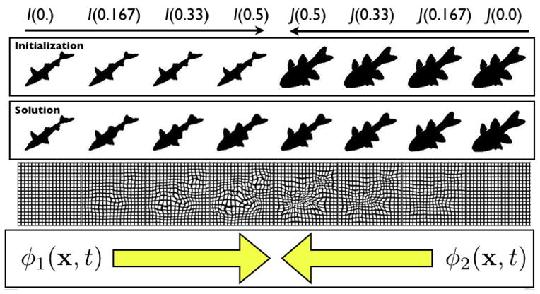
An illustration of a SyN geodesic path between images. The images in the top row are the original images, I and J, at the initialization of the method. After the SyN solution converges, (second row) these images deform in time along the series of diffeomorphisms that connect them. The deforming grids associated with these diffeomorphisms are shown in the bottom row. The maps, φ₁ and φ₂ are of equivalent length and map I and J to the mean shape between the images. The full path, φ and φ⁻¹, are found by joining the paths φ₁ and φ₂. The symmetric nature of this problem (proven in [40]) is due to the interchange-ability of the labels I and J in our problem formulation.

Define the image registration optimization time, t ∈ [0, 1] where t indexes both φ₁ and φ₂, though in opposite directions. The similarity seeks φ₁ such that φ₁(x, 1)I = J. Recalling the basic definition of diffeomorphisms allows us to write any geodesic through composing two parts, each of which is a geodesic (any sub-part of a geodesic is a geodesic). We apply this fact in the second step of our derivation below,

$$\begin{array}{r}{\phi }_1(\mathbf{x},1)I=J,\\ {\phi }_2^{-1}({\phi }_1(\mathbf{x},t),1-t)I=J,\\ {\phi }_2({\phi }_2^{-1}({\phi }_1(\mathbf{x},t),1-t),1-t)I={\phi }_2(\mathbf{z},(1-t)J,\\ {\phi }_1(\mathbf{x},t)I={\phi }_2(\mathbf{z},1-t)J,\end{array}$$ (2)

which converts the similarity term from |φ₁(x, 1)I − J| to |φ₁(x, t)I − φ₂(z, 1 − t)J|². A visualization of these components of φ is in Figure 1. The forward and backward optimization problem is then, solving to time t = 0.5,

$$\begin{array}{r}{E}_{\mathit{sym}}(I,J)=\underset{{\phi }_1}{inf}\hspace{0.17em}\hspace{0.17em}\hspace{0.17em}\underset{{\phi }_2}{inf}\hspace{0.17em}\hspace{0.17em}\hspace{0.17em}{\int }_{t=0}^{0.5}\left\{\right||{\mathit{\upsilon }}_1(\mathbf{x},t)|{|}_L^2+\left|\right|{\mathit{\upsilon }}_2(\mathbf{x},t)\left|{|}_L^2\right\}dt+\\ {\int }_{\mathrm{\Omega }}|I({\phi }_1(0.5))-J({\phi }_2(0.5)){|}^{2}d\mathrm{\Omega }.\\ \text{Subject\hspace{0.17em}to\hspace{0.17em}each\hspace{0.17em}}{\phi }_i\in {\mathit{Diff}}_0\hspace{0.17em}\text{the\hspace{0.17em}solution\hspace{0.17em}of}:\\ d{\phi }_i(\mathbf{x},t)/dt={\mathit{\upsilon }}_i({\phi }_i(\mathbf{x},t),t)\hspace{0.17em}\text{with}\\ {\phi }_i(\mathbf{x},0)=\mathbf{I}\mathbf{d}\hspace{0.17em}\text{and\hspace{0.17em}}{\phi }_i^{-1}({\phi }_i)=\mathbf{I}\mathbf{d},{\phi }_i({\phi }_i^{-1})=\mathbf{I}\mathbf{d}.\end{array}$$ (3)

Minimization with respect to φ₁ and φ₂ provides the symmetric normalization (SyN) solution and also solves a 2-mean problem. Landmarks may also be included, as in the Lagrangian Push Forward method [39], by dividing the similarity term, as done with the image match terms above. The constraint D(φ₁(x, 0.5)) = D(φ₂(x, 0.5)) is built into the fact that we integrate the solution from 0 to 0.5. Because the velocities are of (approximately) constant arc length and are, at each iteration, of exactly the same length, the length of φ₁, integrated over [0, 0.5], is equivalent to the length of φ₂ integrated over [0, 0.5].

As noted in the introduction, this method is quite distinct from inverse consistent image registration (ICIR) [41]. ICIR uses vector fields, h and g, to define correspondence from I to J and J to I, respectively. Therefore, in total, ICIR uses four vector fields in its approach to normalization, h, g, h⁻¹ and g⁻¹. The inverses of these fields are not guaranteed to exist (as the optimization is not performed in the diffeomorphic space) and no exact method is used to compute the inverses. Instead, judging from the brief discussion in [41], the inverse is only guaranteed to be exact at a few points in the domain and the inversion algorithm itself is not well-specified or exact. This inexactness means that the variational term measuring the difference between two vector fields, ||h(x)−g⁻¹(x)||², only coarsely estimates consistency. Furthermore, this means that ICIR must include two terms to compute consistency, that is, both ||h(x)−g⁻¹(x)||² and ||h⁻¹(x)−g(x)||². If inverses were exact (or very close to exact) only one of the above terms would be enough as minimizing one would imply minimizing the other.

SyN, alternatively, provides an inverse that is guaranteed to be everywhere sub-pixel accurate. Furthermore, SyN avoids a basic computational redundancy present in ICIR - the solutions h(x) and g(x) overlap in time. SyN’s pair of solutions, φ₁ and φ₂, on the other hand, do not overlap in time. They are only two parts of a longer path. This distinction is shown in figure 2. However, SyN is still able to compute the measure of inverse consistency by simply composing our time 0.5 maps together and comparing φ₁(x, 1) and ${\phi }_2^{-1}(\mathbf{x},1)$ in the I domain (a similar computation may be done in the J domain). Recall that, by definition and diffeomorphic computations, we are able to guarantee ${\phi }_1^{-1}({\phi }_1)=\mathbf{I}\mathbf{d}$ and ${\phi }_2^{-1}({\phi }_2)=\mathbf{I}\mathbf{d}$. We therefore have an inverse consistency error of zero, up to the inaccuracy induced by the single interpolation required in computing the time 1 maps, e.g. ${\phi }_1(\mathbf{x},1)={\phi }_2^{-1}({\phi }_1(\mathbf{x},0.5),0.5)$. A key to the symmetry of our method is the ability to compute sub-pixel accurate inverses such that, for each i = 1, 2, we have (to a user-selected numerical precision) ${\phi }_i^{-1}({\phi }_i)=\mathbf{I}\mathbf{d}$ and ${\phi }_i({\phi }_i^{-1})=\mathbf{I}\mathbf{d}$. Typical precision is 1.0 × 10⁻⁶ L₁ norm and 0.2 L_∞ norm, measured in terms of voxel/pixel coordinates. Further details on the numerical methods employed in optimizing this energy may be found in [39] and will be summarized below.

Fig. 2.

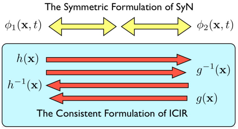
The symmetric normalization method is represented, at top, by its two components, φ₁ and φ₂, meeting at the middle of the normalization domain. Note that each sub-path may be traversed either from the middle to the end or from an end to the middle. Alternatively, the ICIR method is shown in a schematic at the bottom panel of the figure. The correspondence defining vector fields associated with ICIR are called h and g. In ICIR, all four deformation fields overlap in time and may, in fact, be different from each other. The inverse of h may not be its true inverse. Further, the inverse of h may not be equivalent to g.

2.3 The Cross Correlation with Symmetric Diffeomorphisms

We now propose to symmetrically solve the following image matching problem: Find a spatiotemporal mapping, φ ∈ Diff₀, such that the cross correlation between the image pair is maximized. This formulation of the problem represents a change of philosophy when compared to Bajcsy [10] and, later, Gee’s [11] elastic matching, which also used cross-correlation. Elastic image registration methods seek to balance a regularization term and a similarity term allowing one to find a constrained deformable solution. The approach recommended here departs from this strategy by allowing an unconstrained optimization of the similarity term within the space of diffeomorphisms. This strategy is used when finding optimal mappings in lower-dimensional (e.g. affine) transformation groups. The main advantage of an unconstrained search within the space of diffeomorphisms is its simplicity: one allows the method to maximize the similarity until a local maximum or limit on computation time is reached. ² The disadvantage is one requires a similarity metric that, when optimized in Diff, provides a useful solution. Therefore, design and choice of the similarity metric requires great care.

The mutual information (MI) similarity metric garnered significant interest in recent years [42,43,14,44]. Intuitively speaking, MI estimates the optimal matching between images by inferring how much global information is shared in the image pair, as estimated from the pair’s joint histogram. At the same time, MI prevents over-fitting by penalizing clustering of the marginal image probabilities [31]. The globality of this approach makes it extremely useful for robust rigid registration but may limit performance in deformable registration, in particular in cases where non-stationary noise patterns or intensity inhomogeneity requires a locally adaptive similarity. This problem has been addressed by Studholme et al [44] and in our previous work [45]. One difficulty with a locally varying estimate to the MI is that joint probabilities need a large number of samples for reliable statistics. Therefore, as locality in the MI estimate increases, its statistical reliability decreases.

Cross-correlation (CC), on the other hand, adapts naturally to situations where locally varying intensities occur and is suitable for some multi-modality problems. The CC depends only on estimates of the local image average and variance which may be accurately/exactly measured with relatively few samples. Furthermore, the cross-correlation has shown historically to perform well in many real-world computer vision applications where one requires robustness to unpredictable illumination, reflectance, etc. An example of the robustness of our method to strong MRI inhomogeneity (bias field) is shown in figure 3. For these reasons, we revisit the classical cross-correlation as a similarity metric for use in our emerging diffeomorphic image registration.

Fig. 3.

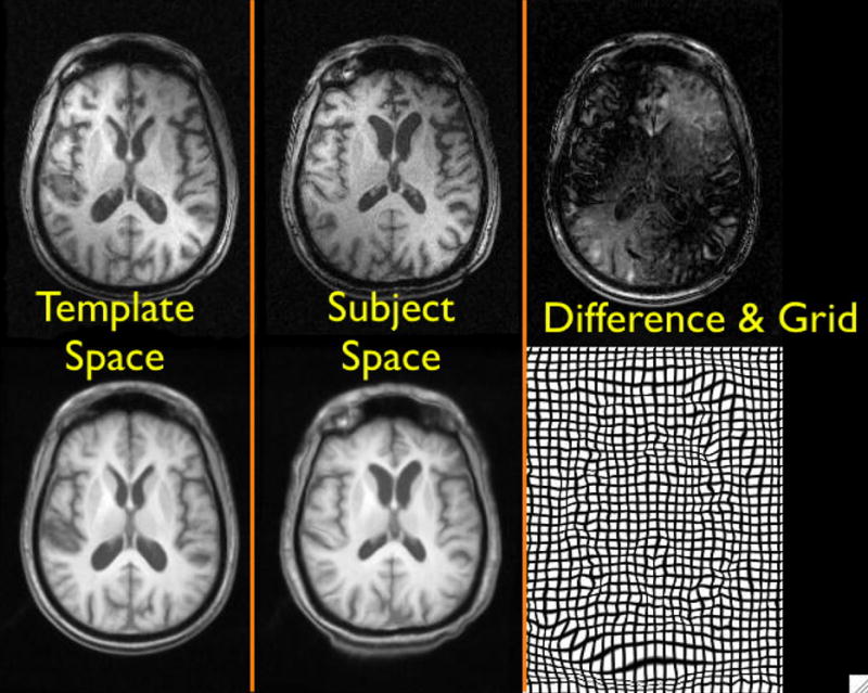
The local cross correlation measure allows robust matching of images despite the presence of a strong bias field affecting the image quality. The smoothness of the grid is also unaffected by the bias.

We now provide a symmetric formulation of the diffeomorphic image registration problem as driven by CC, along with the Euler-Lagrange equations for this problem. First, define I₁ = I(φ₁(x, 0.5)) and J₂ = J (φ₂(x, 0.5)). We also define a variable to represent each image with its local mean subtracted as Ī(x) = I₁(x) − μ_I1 (x) and J̄(x) = J₂ − μ_J2 (x). We compute μ over a local n^D window centered at each position x, where D is the image dimension. We usually choose n = 5. The cross-correlation is then

$$CC(\overline{I},\overline{J},\mathbf{x})=\frac{<\overline{I},\overline{J}{>}^2}{<\overline{I}><\overline{J}>}=A^2/BC,$$ (4)

where the inner product is also taken over a n^D window. Note that our CC is implicitly a function of φ₁ and φ₂ through its dependence on I₁ and J₂. We now are able to define the variational optimization problem in similar fashion to equation 3,

$$\begin{array}{r}{E}_{CC}(\overline{I},\overline{J})=\underset{{\phi }_1}{inf}\hspace{0.17em}\hspace{0.17em}\hspace{0.17em}\underset{{\phi }_2}{inf}\hspace{0.17em}\hspace{0.17em}\hspace{0.17em}{\int }_{t=0}^{\frac{1}{2}}\left\{\right||{\mathit{\upsilon }}_1(\mathbf{x},t)|{|}_L^2+\left|\right|{\mathit{\upsilon }}_2(\mathbf{x},t)\left|{|}_L^2\right\}dt+\\ {\int }_{\mathrm{\Omega }}CC(\overline{I},\overline{J},\mathbf{x})d\mathrm{\Omega }.\\ \text{Subject\hspace{0.17em}to\hspace{0.17em}each\hspace{0.17em}}{\phi }_i\in {\mathit{Diff}}_0\hspace{0.17em}\text{the\hspace{0.17em}solution\hspace{0.17em}of}:\\ d{\phi }_i(\mathbf{x},t)/dt={\mathit{\upsilon }}_i({\phi }_i(x,t),t)\hspace{0.17em}\text{with}\\ {\phi }_i(\mathbf{x},0)=\mathbf{I}\mathbf{d}\hspace{0.17em}\text{and\hspace{0.17em}}{\phi }_i^{-1}({\phi }_i)=\mathbf{I}\mathbf{d},{\phi }_i({\phi }_i^{-1})=\mathbf{I}\mathbf{d}.\end{array}$$ (5)

The problem, here, is the same as before but with the cross-correlation as the driving similarity term. We now take the variation of this function with respect to φ₁ at time 0.5 and φ₂ at time 0.5. Following Beg’s derivation, adapted for our symmetric normalization and particular similarity metric, we find two Euler-Lagrange equations,

$${\nabla }_{{\phi }_1(\mathbf{x},0.5)}{E}_{CC}(\mathbf{x}),=2L{\mathit{\upsilon }}_1(\mathbf{x},0.5)+\frac{2A}{BC}(\overline{J}(\mathbf{x})-\frac{A}{B}\overline{I}(\mathbf{x}))\left|D{\phi }_1\right|\nabla \overline{I}(\mathbf{x}),$$ (6)

$${\nabla }_{{\phi }_2(\mathbf{x},0.5)}{E}_{CC}(\mathbf{x}),=2L{\mathit{\upsilon }}_2(\mathbf{x},0.5)+\frac{2A}{BC}(\overline{I}(\mathbf{x})-\frac{A}{C}\overline{J}(\mathbf{x}))\left|D{\phi }_2\right|\nabla \overline{J}(\mathbf{x}).$$ (7)

The gradients given in equations 6 and 7 include that fact that the velocities exist in the space of smooth vector fields given by the linear operator L as well as the determinant of each φ_i transformation Jacobian, |Dφ_i|. This equation is similar to both that derived for LDDMM [23] and the derivative for the cross-correlation given by Hermosillo [31]. This equation differs from Beg’s Euler-Lagrange equation in that we have an E-L equation for both φ₁ and φ₂ instead of just φ₁. In addition, Beg used the intensity difference metric given in equation 3. The derivation of this equation differs from that in Hermosillo [31] by the presence of the derivative of the diffeomorphism ∂Ī/∂φ_i, which leads to the Jacobian term, instead of a vector field (small deformation) derivative. Furthermore, we have represented the CC in a different arrangement of terms that suits our own derivation of the CC variation and computational implementation. This arrangement of terms allows one to precompute, for each iteration, the locally varying values of A, B, C and store them for use in the local computation of the derivative.

Our novel symmetric formulation, therefore, does not add significant additional cost to the normalization. The main additional cost is that of smoothing the derivative estimate to gain the υ_i, not in the actual estimate of the similarity term. Both the φ₁ and φ₂ derivatives require the terms A, B and C. Therefore, in estimating equation 6 and equation 7, we use the procedure detailed in algorithm 1 below.

Algorithm 1 : Computing Cross-Correlation Derivatives

(1) Deform I by φ₁(0.5) and J by φ₂(0.5).

(2) Calculate Ī and J̄ from the result of step (1).

(3) Calculate and store images representing A, B and C.

These steps enable us to loop over the image domain to rapidly compute equation 6 and equation 7 at the same time from these precomputed variables. Note, however, that it could be possible to modify Lewis’s fast normalized correlation measure [46] to speed up this process even further.

Equations 6 and 7 gives the update to the velocities at time 0.5 and consequently the diffeomorphisms φ₁ and φ₂. However, we also require the φ_i to satisfy our o.d.e. and exact invertibility constraints. We satisfy these constraints by, given a new velocity estimate, first updating the φ_i through the o.d.e. and then integrating backward in time to find φ_i ⁻¹ and verify invertibility. This approach is a standard one and detailed, algorithmically, in the LPF method [39]. For completeness, we include an abbreviated explanation here.

First, assume arbitrary φ and υ, related by the standard o.d.e. dφ(x, t)/dt = υ(φ(x, t), t) used to generate diffeomorphisms. The update method for our diffeomorphism comes from discretization of this o.d.e., such that,

$$\phi (\mathbf{x},t+\mathrm{\Delta }t)\leftarrow \phi (\mathbf{x},t)+\mathrm{\Delta }t\mathrm{\hspace{0.17em} }\mathit{\upsilon }(\phi (\mathbf{x},t),t).$$ (8)

This discretization is used to update both φ_i from time 0 to 0.5. Second, algorithm 2 gives a method for generating inverses when an arbitrary diffeomorphism φ is updated by a small time-step through a velocity field, as in the previous equation. The algorithm typically converges within one to a few iterations, particularly if the time step is small. The existence of a solution is guaranteed by the integrability condition established for diffeomorphic image registration [19], while uniqueness comes from the uniqueness theorem of o.d.e.s [36].

Algorithm 2 : Inversion Method

The algorithm uses a fixed point method to push the inverse of φ forward by a small amount performing a gradient descent on φ⁻¹(φ) = Id, enforcing φ⁻¹(φ) = Id to a sub-pixel level. The same approach was used in the Lagrangian Push Forward algorithm [39]. We use a temporary variable, ψ, to represent the input di3eomorphism that, on output, will be the inverse of φ. Input φ(x) = y, ψ⁻¹(ỹ) = x where ỹ ≠ y and output ψ⁻¹(y) = x = φ⁻¹(y). At convergence, ỹ = y and ||ψ⁻¹(φ) − Id||_∞ < ε₂r where r is the image resolution and ε₂ a small constant, typically 0.1.

1: while ||ψ⁻¹(φ(x)) − x||_∞ > ε₂r do

2: Compute ν⁻¹(x) = ψ⁻¹(φ(x)) − x.

3: Find scalar γ such that ||ν⁻¹||_∞ = 0.5r.

4: Integrate ψ⁻¹ s.t. ψ⁻¹(ỹ, t)+ = γ ν⁻¹(ψ⁻¹(ỹ, t)).

5: end while

We now summarize the SyN method in algorithm 3. Our implementation essentially updates each φ_i with the current estimate to the velocity, follows the update to each φ_i by calling algorithm 2 to generate inverse maps, and then re-estimates the velocity from the new estimate to the φ_i. This formulation and diffeomorphic representation guarantee SyN’s sub-pixel invertibility and algorithmic independence to input permutations. These methods allow us to symmetrically match images to the degree that discrete diffeomorphisms are invertible. Furthermore, while extended here to cross-correlation, similar techniques may be used to efficiently symmetrize almost any other similarity measure. We now leverage ITK for a fair implementation and evaluation of SyN.

Algorithm 3 : Overview of Symmetric Normalization Method

(1) Initialize ${\phi }_1=\mathbf{I}\mathbf{d}={\phi }_1^{-1}$ and ${\phi }_2=\mathbf{I}\mathbf{d}={\phi }_2^{-1}$.

(2) Repeat the following steps until convergence:

(3) Compute the cross correlation as described in algorithm 1.

(4) Compute each ν_i by smoothing the result of step (3) in this table. One may also use the modified midpoint method for each velocity, as in the LPF algorithm [39], to give smoothness in time.

(5) Update each φ_i by ν_i through the o.d.e. as described in equation 8. This step automatically adjusts the time step-size such that the maximum length of the updates to the φ_i is sub-pixel and approximately constant over iterations. We explicitly guarantee ||ν₁(·, t) || = ||ν₂(·,t) ||. We also update the estimate to the geodesic distance by trapezoidal rule, as in the LPF method.

(6) Use algorithm 2 to get the inverses of the φ_i.

(7) Generate the time 1 solutions from ${\phi }_1(1)={\phi }_2^{-1}({\phi }_1(\mathbf{x},0.5),0.5)$ and ${\phi }_1^{-1}(1)={\phi }_2(1)={\phi }_1^{-1}({\phi }_2(\mathbf{x},0.5),0.5)$.

2.4 Implementation in ITK

The Demons algorithm is freely available in the standard ITK distribution and has been quantitatively evaluated by the ITK community. We have implemented SyN within our extended version of the ITK deformable image registration framework, described in [47]. Therefore, we are in a position to measure performance gains by varying first the similarity metric and then the the transformation model, keeping an identical underlying code base.

Switching the Similarity Metric

For this part of the study, we replace the itkDemonsRegistrationFunction, in the itkDemonsRegistrationFilter, with our own itkCrossCorrelationRegistrationFunction. The interface and operation of this modified deformable registration algorithm are identical to the Demons algorithm, except that the image forces come from the small deformation version of equation 6, as may be found in [31]. In addition to switching the itkDemonsRegistrationFunction for our cross-correlation image forces, we also modified the time step used during this elastic registration process. The time-step was increased from 1, for Demons, to 4 for cross-correlation. The Demons force, based on optical flow, is extremely aggressive compared to our analytical cross-correlation derivative. We found, for our dataset, that time-steps beyond 4 led to non-positive Jacobians in a significant fraction of our normalizations.

Switching the Transformation Model

As mentioned previously, we have implemented SyN in our extended Insight ToolKit. For this study, SyN will use the itkPDEDeformableRegistrationFilter as implemented in ITK for its Gaussian smoothing operator ³. This smoothing operator will be applied only to the incremental output of our itkCrossCorrelationRegistrationFunction. The Demons and elastic cross-correlation algorithms both apply Gaussian smoothing to the total displacement field, in accordance with small deformation transformation models. The presence of a large deformation assumption, along with the use of a space-time parameterization of the transformation, are the main (not the only) differences between diffeomorphic and elastic registration algorithms.

The key contrast between the first pair of methods (Demons, elastic cross-correlation) is the similarity metric. The only difference between the second two (elastic cross-correlation, SyN cross-correlation) is in the transformation model. We are therefore investigating, first, if cross-correlation provides better normalization than Demons optical flow, for our neurodegenerative and elderly T1 MRI dataset. The second comparison evaluates if changing from the elastic to the symmetric diffeomorphic transformation model yields additional improvement. Our hypothesis was that each change would yield benefits. This hypothesis was born out in our experimental data, as suggested by the preliminary study data shown in figure 4.

Fig. 4.

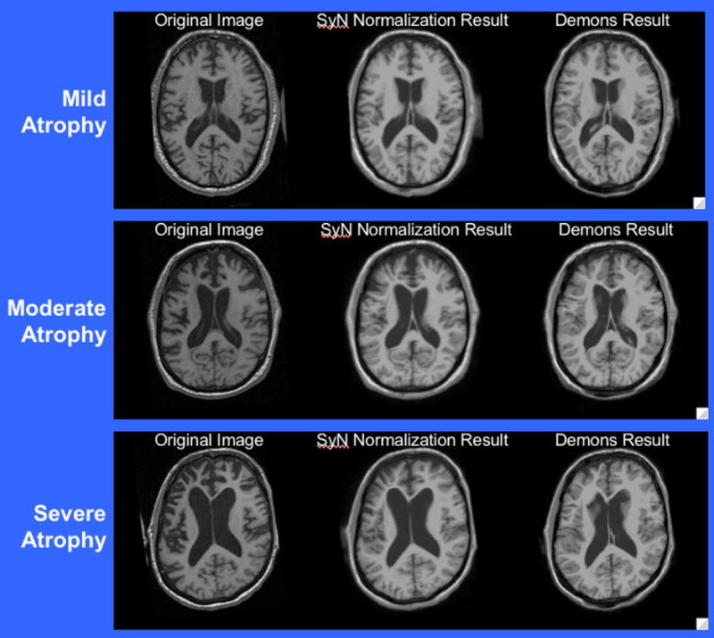
The atlas was initially aligned to these FTD images via a rigid plus uniform scaling transformation. The subsequent Demons registration to each image, used for labeling, is in the right column. The SyN result is in the center column, while the corresponding original images are in the left column. The Demons method does a reasonable normalization, but leaves the ventricles and other smaller structures only partly normalized. The quadratic elastic penalty prevents the remaining shape differences from being captured. A similar loss of resolution in the mapping is seen in the elastic cross-correlation mappings. These are illustrative images from our previous study, [49], and were not used as actual study data in this exposition.

3 Data and Experiments

Dataset

Our database consists of 20 T1 MRI images (0.85 × 0.85 × 1.5 mm, GE Horizon Echospeed 1.5 T scanner) from 10 normal elderly and 10 frontotemporal dementia patients. The 10 frontotemporal dementia individuals are a different set than used in our previous study [49]. Each of the 20 images, along with the elderly template, was manually labeled with the protocol described in [8]. This protocol was shown to be highly reproducible for both small and large structures via six-month intra-rater reliability and inter-rater reliability measurements. Left hippocampus labeling, for example, showed a 0.92 intra-rater overlap ratio (equation 1) and 0.83 average for inter-rater overlap. As the hippocampus is relatively small, these values are reasonable. Finally, as the labeling was intended to be only on the cortex (not cerebrospinal fluid), we masked the label images by the inverse of the cerebrospinal fluid segmentations. This also makes our evaluation more sensitive to differences in the accuracy of sulcal and gyral alignment.

Evaluation

We now use these two comparative pairings of three algorithms to study performance for characterizing the volumetric differences between elderly and frontotemporal dementia cortex, hippocampus, amygdala and cerebellum. An example comparison of the SyN and Demons methods’ normalization abilities is in figure 4. This study reveals the ability of these methods, SyN, elastic cross-correlation and Demons, to reproduce results gained from an expert user’s labeling of our 20 image dataset. This test is performed by using each method to map the template labels (an elderly individual also labeled by our expert user) to each individual. Twenty rigid registrations and sixty non-rigid registrations were required (twenty subjects were each deformably registered by three algorithms). The atlas labelings are then warped by the composed rigid and non-rigid transformation into the space of the patient image. We then compute Dice overlap ratios between the manual and automatic structural segmentations for each structure.

Each method was applied in an identical four-level multi-resolution scheme and ran until convergence or a fixed (maximum) number of iterations was reached. We allowed up to 100 iterations at the first level, 100 iterations at the second level, 100 iterations at the third level and 20 iterations at the full resolution. The relative running times for each algorithm varied depending upon the particular cases being run. However, the relative average running times (in terms of the average Demons running time) were 1 (Demons), 4.2 (elastic cross-correlation) and 5.5 (SyN). The mean runtime of the Demons method on a 2.0 GHz Intel Mobile Pentium processor was 20.4 minutes. The relative similarity of the elastic time cost to the cost of SyN also indicates that our symmetric approach does not create significant additional computational cost.

4 Results and Discussion

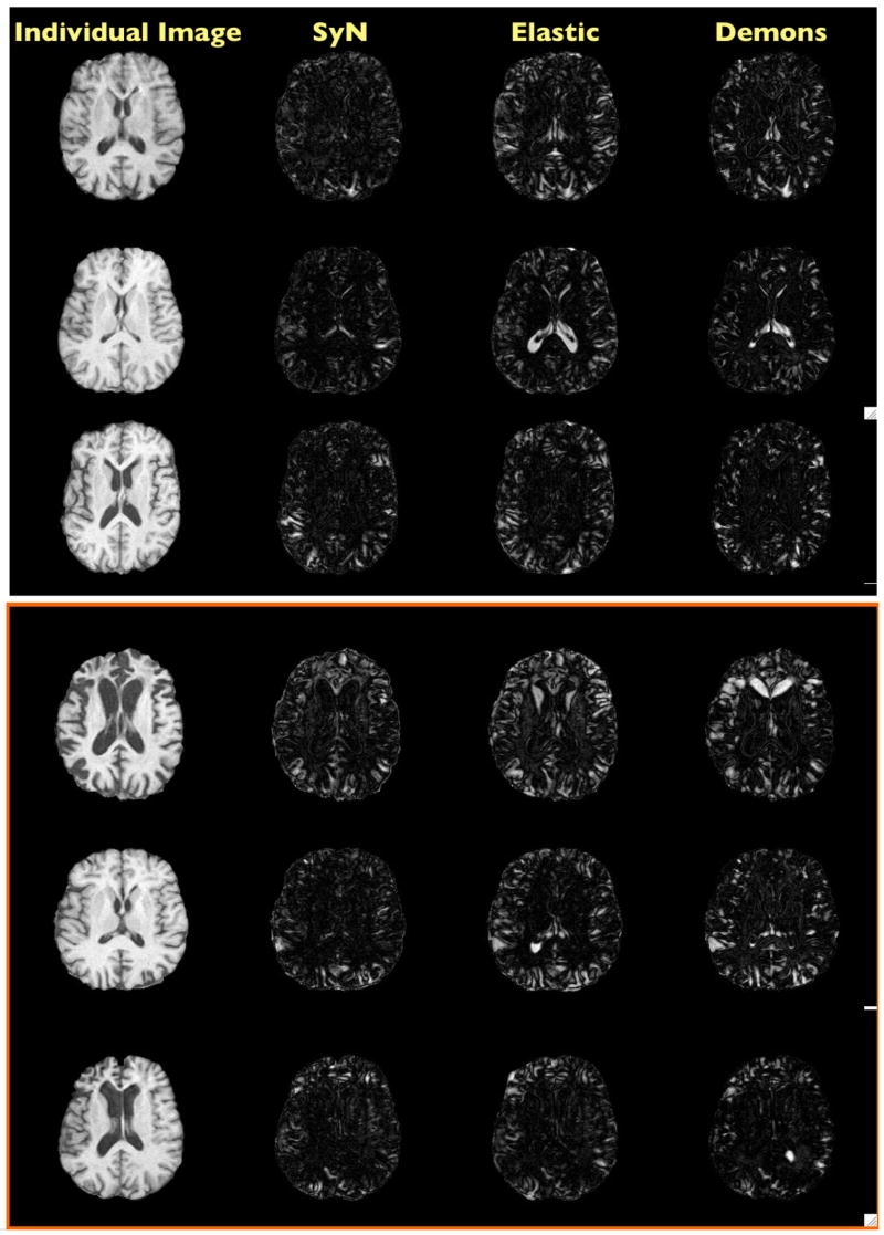
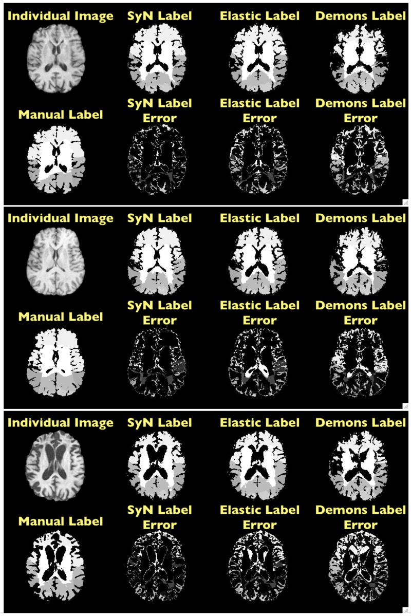
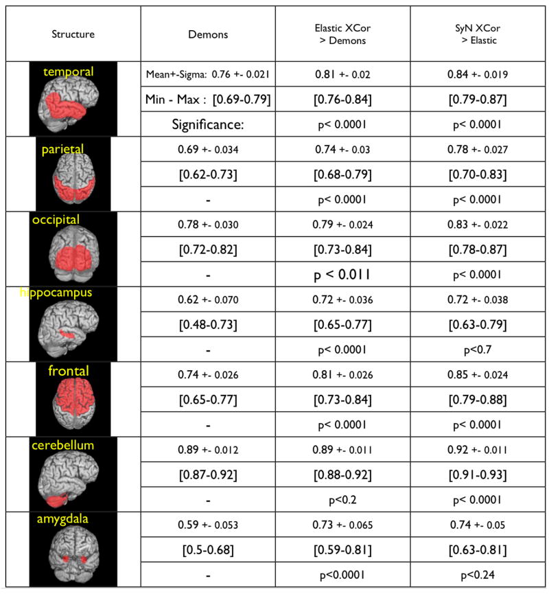
A visualization of six individuals from our dataset and the normalization of the template to these individuals is shown in figure 5. Associated intensity error images are shown in figure 6. Label error images are shown in figure 7. The eight labeled individual structures are shown, along with the summary statistics for our results, in figure 8. Both cross-correlation algorithms produced segmentation results above the minimum threshold of 0.6 for all structures, as shown in figure 8. We also compared the minimum Jacobian of the elastic cross-correlation and SyN cross-correlation methods and did not find significant differences (T= −1.67725, P < 0.101703). This indicates that SyN’s results are not significantly less constrained at a local level. The smallest difference in performance between the Demons and elastic cross-correlation methods was on the cerebellum. The highest difference was on the frontal lobe. The largest performance difference in SyN and elastic cross correlation was on the temporal and frontal lobe. Performance gains expectedly focus on frontal and temporal lobe due to the known effect of FTD on these two areas. The shape changes caused by this complex disease are likely difficult to capture with a constrained method such as elastic normalization. The smallest differences between the elastic and diffeomorphic methods were found in the hippocampus and amygdala. This is likely to indicate that the similarity metric does not provide a rich enough feature space over which to optimize the correspondence of these structures. Therefore, a better optimizer operating with that similarity metric will not be likely to provide an advantage.

Fig. 5. Normalization Results.

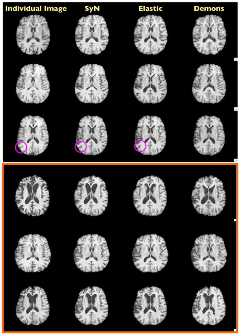
All images in each row should look similar to the first image in the row. The atlas was initially aligned to these elderly (top three) and FTD (bottom three) images via a rigid plus uniform scaling transformation. These examples are from our current study. We have highlighted (with a circle) the type of small scale difference one may see in the registration quality. Larger scale differences are also clear. In particular, the Demons and elastic cross-correlation have problems both shrinking and expanding the ventricles (the second elderly image). In addition, the Demons intensity consistency assumption causes significant errors in the first FTD image, a case where this assumption does not hold.

Fig. 6. Normalization Results Difference Images.

This figure shows the same results as figure 4, but with absolute value of the image difference, after normalization. One can observe that small sulci may not be captured by any of the methods. Under the intensity difference metric, the Demons method should be expected to perform best, as it explicitly minimizes this error.

Fig. 7. Normalization Results Label Error Images.

Here, we show three individual images along with the manual, SyN, elastic and Demons labels. This bottom row for each individual shows the difference of the algorithmic and manual labels. The majority of the errors are due to a shift or a curvature in the boundary definition gained algorithmically, with respect to the manual definition. Manually defined lobar boundaries tend to be planar. Further, when one compares the (in particular, parietal) boundaries determined by the labeler on these three images, it becomes apparent that there may be some inconsistency. Secondary errors are due to lack of sulcal definition in the template labels, with respect to the individual labeled ground truth.

Fig. 8. Performance comparison and average Dice statistic for each method and each structure.

Example brain labelings mark the structures over which we evaluated the three algorithms. The final results showed that, overall, SyN > Elastic > Demons for automatically labeling these lobar structures. The P-values for the difference in performance were computed using non-parametric permutation testing based on the paired T-test on vectors of Dice statistics. We used 10,000 permutations per example, thus limiting our minimum P-value to 0.0001. Extremely small P-values indicate that the method uniformly and strongly outperformed the method with which it was paired.

A likely improvement in performance would come from using a method such as the STAPLE algorithm [50] to bootstrap results. Similarly, an optimal template would augment results [51]. However, both of these enhancements would increase performance in a consistent manner across all our tested registration methods and would be unlikely to change the relative performance of our algorithms.

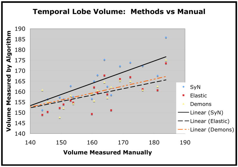
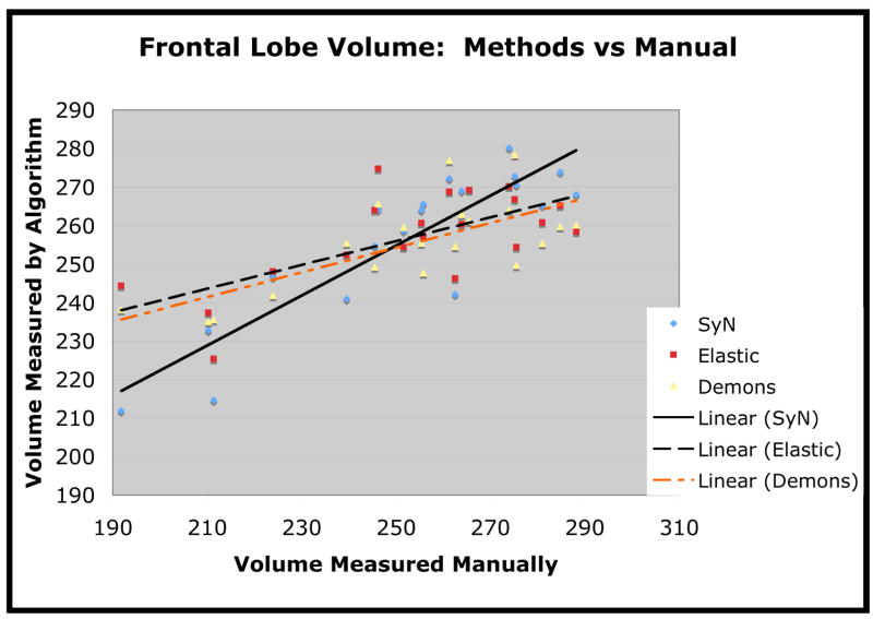
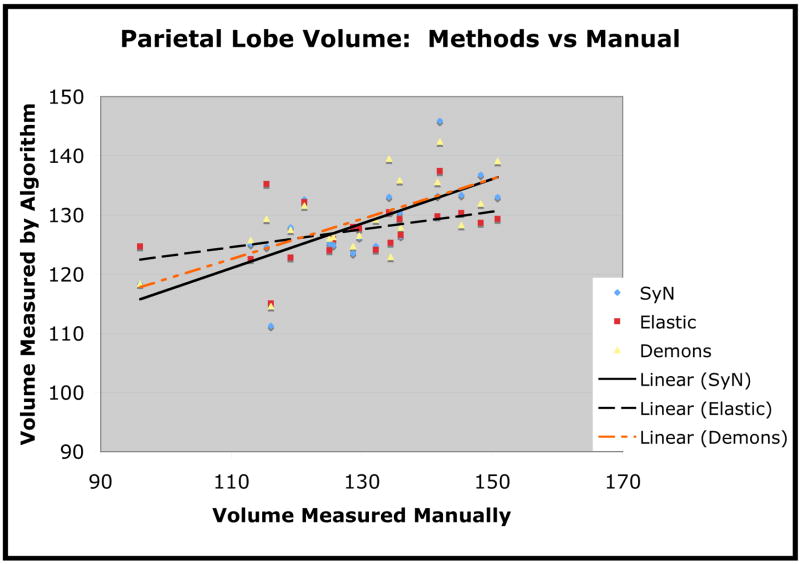
The second test we performed was to evaluate whether the volume measurements obtained by the normalization are strongly correlated with the measurements of the expert user. We performed this analysis only on regions (frontal, temporal, parietal lobes) where one may reasonably expect FTD to induce a difference from the normal Elderly population and where labeling performance was good. The purpose of this test is to determine if conclusions made by analyzing the output of our automated normalization methods are at all consistent with the expert user’s analysis. As we are using the expert labeling as our gold standard, the “better” method should produce volume measures that correlate more strongly with the volume measures gained by the expert. The volume, in cubic centimeters, of each structure was calculated by summing the voxel volumes that were given the appropriate label for that structure. As shown in table 1, SyN outperformed elastic cross-correlation (and the Demons method) according to the degree to which the automated volumes correlate with the manual volumes for each of three structures. SyN also had the least overall discrepancy in the measured volume, that is, Σ_i |V_Alg − V_Man|, where V_Man is manually measured volume and V_Alg refers to algorithmically measured volume. These results are shown in table 2.

Table 1.

Pearson correlations between manual and algorithmic volume measures.

Structure	Corr(Man,Syn)	Corr(Man,Elas)	Corr(Man,Demons)
Temporal	0.86	0.69	0.79
Frontal	0.89	0.67	0.71
Parietal	0.71	0.42	0.66

Table 2.

The average absolute volume error between manual volume and algorithmic volume measured over the dataset for each structure.

Structure	VolErr(Man,Syn)	VolErr(Man,Elas)	VolErr(Man,Demons)
Temporal	8.4	9.2	8.7
Frontal	11.1	16.1	15.8
Parietal	7.9	9.3	7.9

We also plot the estimated volume versus the manually computed volume for the temporal lobe in figure 9, for frontal lobe in figure 10 and for parietal lobe in figure 11. We use linear regression to fit the estimated volume with a line in order to assess the closeness of the method’s estimate to the manual estimate. The Pearson correlation of SyN volumes with the manually measured volumes was 0.86 for temporal lobe, 0.89 for frontal lobe and 0.71 for parietal lobe. The correlation of the elastic method volumes with the manually measured volumes was 0.69 for temporal lobe, 0.67 for frontal lobe and 0.42 for parietal lobe. The correlation of Demons volumes with the manually measured volumes was 0.79 for temporal lobe, 0.67 for frontal lobe and 0.66 for parietal lobe. One interesting finding, here, is that the Demons method, compared to the elastic method, produces stronger correlations with manual labelings (in terms of volume measurements) but produces smaller overlap ratios.

Fig. 9.

Temporal lobe volume, in cubic centimeters, as measured by each of the three methods. The algorithmic measures are plotted against the manually measured volume.

Fig. 10.

Frontal lobe volume, in cubic centimeters, as measured by each of the three methods. The algorithmic measures are plotted against the manually measured volume.

Fig. 11.

Parietal lobe volume, in cubic centimeters, as measured by each of the three methods. The algorithmic measures are plotted against the manually measured volume.

Our final analysis tests the significance of the difference in volumes between the FTD and elderly members of our image population. The P-values of these results, obtained by non-parametric permutation testing, are shown in table 3. None of the structures showed a significant volumetric difference between groups. However, SyN appears to reflect the significance obtained by the manual rater more closely than the other methods. At the same time, we do not find these results to be strong enough to warrant definitive conclusions. Comparing a larger dataset (or possibly a different set of control and subject images) would likely show stronger differences than this dataset, as we found in our previous, preliminary study [49].

Table 3.

Significance of Elderly-FTD volume differences as measured by manual, SyN, elastic and Demons methods. Significance was determined by a permutation test based on the unpaired T-test of Elderly and FTD structure volumes.

Structure	Eld-FTD Man.	Eld-FTD SyN	Eld-FTD Elas.	Eld-FTD Demons
Temporal	0.25	0.35	0.47	0.26
Frontal	0.18	0.13	0.49	0.52
Parietal	0.32	0.46	0.82	0.15

Contrasting Automated and Manual Results

Thus, we can see how an apparently small, but consistent difference in performance (as measured by overlap ratio) can have an impact on the validity of the study outcome. That is, the performance gains in overlap ratio translate to more accuracy in making clinically meaningful measurements, such as volume. Although the quality of our results are reasonable, by some standards, these algorithms, as applied here, cannot claim to accurately reproduce manual labelings. The reasons for this are well-known. The primary reason is that expert knowledge is not directly encoded in these methods. Secondarily, the uncertainty inherent to the problem of neuroanatomical labeling limits the accuracy and reproducibility of both manual and automated segmentation. Finally, it is not yet known the extent to which brains of different individuals, when represented as magnetic resonance images, are diffeomorphic to each other. This problem is even less well understood with elderly and patient brains. Note also that, when measuring the trends in the difference of elderly and FTD structure volumes, the Demons, elastic correlation and SyN significance tend to estimate larger volumes than the manual results. This is likely caused by two things: segmentation bias towards the template and the fact that registration-based segmentations are smoothed (elastic and Demons more than SyN), while the manual segmentations are not. Both of these types of errors may be observed in figure 7. Figure 7 also shows that the labeler may have used different “styles” of labeling or changed the decision-making process over the dataset. All of these confounds impact the overlap ratios and correlations that we find here. We accentuate that our goal, here, is not specifically to reproduce the expert labels, but to use these labeled structures as a neuroanatomically-based evaluation of relative algorithmic performance.

5 Conclusion

We first described the symmetric normalization formulation. We then extended this formulation to use the cross-correlation similarity function providing, in addition, Euler-Lagrange equations for the variational problem in the symmetric diffeomorphic context. We contrasted our method with the popular inverse consistent image registration technique, which was outperformed by the Demons method in an unbiased comparative evaluation of brain segmentation and alignment [32]. We then provided algorithmic details of the SyN methodology. Finally, we leveraged our ITK implementation to compare the SyN cross-correlation optimizer with the Demons and an elastic cross-correlation optimizer. This enabled us to explore the effect of similarity metric and optimizer separately and purely, as we use an identical linear operator for regularization and an identical code base, the Insight ToolKit. The relative similarity of the elastic computation time to the computational cost of SyN also indicates that our symmetric approach does not require significant additional computational expense. We found, in short, that the cross-correlation behaves well on elderly and neurodegenerative data. In particular, it outperforms the Demons optical flow on our dataset. We also found that the symmetric diffeomorphic optimizer outperforms the elastic optimizer on the same dataset, while guaranteeing that the topology of the images is preserved and, importantly, that the algorithm’s performance does not depend upon the order in which one inputs the images.

This careful comparison establishes the distinct advantage of SyN for segmenting elderly and neurodegenerative cerebrum, cerebellum and, in particular, the temporal and frontal lobe. Note that, in addition to better performance, SyN provides a dense space-time map and transformation inverses. The differences in performance are consistent, statistically significant and have a major impact on study outcome. One can extrapolate even larger differences between SyN and algorithms with lower dimensionality than either Demons or SyN. For this reason, along with the theoretical advantages that translate into practical benefits, we promote diffeomorphic algorithms and the cross-correlation similarity metric in neuroimaging research, in particular when studying nonstandard datasets, such as FTD and AD.

References

- 1.Ratnavalli E, Brayne C, Dawson K, Hodges JR. The prevalence of frontotemporal dementia. Neurology. 2002;58(11):1585–1586. doi: 10.1212/wnl.58.11.1615. [DOI] [PubMed] [Google Scholar]
- 2.Chan D, Fox NC, Jenkins R, Scahill RI, Crum WR, Rossor MN. Rates of global and regional cerebral atrophy in ad and frontotemporal dementia. Neurology. 2001;57(10):1756 – 1763. doi: 10.1212/wnl.57.10.1756. [DOI] [PubMed] [Google Scholar]
- 3.Fox N, Crum W, Scahill R, Stevens J, Janssen J, Rossor M. Imaging of onset and progression of alzheimer’s disease with voxel-compression mapping of serial magnetic resonance images. Lancet. 2001;358:201–205. doi: 10.1016/S0140-6736(01)05408-3. [DOI] [PubMed] [Google Scholar]
- 4.Studholme C, Cardenas V, Blumenfeld R, Schuff N, Rosen HJ, Miller B, Weiner M. Deformation tensor morphometry of semantic dementia with quantitative validation. Neuroimage. 2004;21(4):1387–1398. doi: 10.1016/j.neuroimage.2003.12.009. [DOI] [PubMed] [Google Scholar]
- 5.Kertesz A, Martinez-Lage P, Davidson W, Munoz DG. The corticobasal degeneration syndrome overlaps progressive aphasia and frontotemporal dementia. Neurology. 2004;55:1368–1375. doi: 10.1212/wnl.55.9.1368. [DOI] [PubMed] [Google Scholar]
- 6.Avants B, Grossman M, Gee JC. The correlation of cognitive decline with frontotemporal dementia induced annualized gray matter loss using diffeomorphic morphometry. Alzheimer’s Disease and Associated Disorders. 2005;19(Supplement 1):S25–S28. doi: 10.1097/01.wad.0000183083.14939.82. [DOI] [PubMed] [Google Scholar]
- 7.Ballmaier M, O’Brien JT, Burton EJ, Thompson PM, Rex DE, Narr KL, McKeith IG, DeLuca H, Toga AW. Comparing gray matter loss profiles between dementia with lewy bodies and alzheimer’s disease using cortical pattern matching: diagnosis and gender effects. NeuroImage. 2004;23:325–335. doi: 10.1016/j.neuroimage.2004.04.026. [DOI] [PubMed] [Google Scholar]
- 8.Sparks B, Friedman S, Shaw D, Aylward E, Echelard D, Artru A, Maravilla K, Giedd J, Munson J, Dawson G, Dager S. Brain structural abnormalities in young children with autism spectrum disorder. Neurology. 2002;59:184–92. doi: 10.1212/wnl.59.2.184. [DOI] [PubMed] [Google Scholar]
- 9.Dawant B, Li R, Cetinkaya E, Kao C, Fitzpatrick J, Konrad P. Computerized atlas-guided positioning of deep brain simulators: A feasibility study. In: Gee J, Maintz JB, editors. Workshop on Biomedical Image Registration; Philadelphia. July, 2003; pp. 142–150. [Google Scholar]
- 10.Bajcsy R, Lieberson R, Reivich M. A computerized system for the elastic matching of deformed radiographic images to idealized atlas images. J Comput Assist Tomogr. 1983;5:618–625. doi: 10.1097/00004728-198308000-00008. [DOI] [PubMed] [Google Scholar]
- 11.Gee JC, Reivich M, Bajcsy R. Elastically deforming a 3D atlas to match anatomical brain images. J Comput Assist Tomogr. 1993;17:225–236. doi: 10.1097/00004728-199303000-00011. [DOI] [PubMed] [Google Scholar]
- 12.Gee JC, Bajcsy RK. Elastic matching: Continuum mechanical and probabilistic analysis (Chapter 11) In: Toga AW, editor. Brain Warping. Academic Press; San Diego: 1999. pp. 183–197. [Google Scholar]
- 13.Peckar W, Schnorr C, Rohr K, Stiehl HS, Spetzger U. Linear and incremental estimation of elastic deformations in medical registration using prescribed displacements. Machine Graphics and Vision. 1998;7(4):807–829. [Google Scholar]
- 14.Rueckert D, Sonoda LI, Hayes C, Hill DLG, Leach MO, Hawkes DJ. Nonrigid registration using free-form deformations: Application to breast MR images. IEEE Transaction on Medical Imaging. 1999;18(8):712–721. doi: 10.1109/42.796284. [DOI] [PubMed] [Google Scholar]
- 15.Rogelj P, Kovacic S. Symmetric image registration. Medical Image Analysis. 2006;10(3):484–493. doi: 10.1016/j.media.2005.03.003. [DOI] [PubMed] [Google Scholar]
- 16.Ashburner J, Good C, Friston K. Tensor based morphometry. NeuroImage. 2000;11:465. doi: 10.1006/nimg.2000.0582. [DOI] [PubMed] [Google Scholar]
- 17.Trouv’e A. Diffeomorphism groups and pattern matching in image analysis. Intl J Comp Vis. 1998;28(3):213–221. [Google Scholar]
- 18.Christensen GE, Joshi SC, Miller MI. Volumetric transformation of brain anatomy. IEEE Trans Med Imaging. 1997;16(6):864–877. doi: 10.1109/42.650882. [DOI] [PubMed] [Google Scholar]
- 19.Dupuis P, Grenander U, Miller MI. Variational problems on flows of diffeomorphisms for image matching. Quarterly of Applied Mathematics. 1998;56(3):587–600. [Google Scholar]
- 20.Younes L. Computable elastic distance between shapes. SIAM J Appl Math. 1998;58:565–586. [Google Scholar]
- 21.Joshi SC, Miller MI. Landmark matching via large deformation diffeomorphisms. IEEE Transactions in Image Processing. 2000;9(8):1357–1370. doi: 10.1109/83.855431. [DOI] [PubMed] [Google Scholar]
- 22.Miller M, Trouv’e A, Younes L. On the metrics and Euler-Lagrange equations of computational anatomy. Annu Rev Biomed Eng. 2002;4:375–405. doi: 10.1146/annurev.bioeng.4.092101.125733. [DOI] [PubMed] [Google Scholar]
- 23.Beg F, Miller M, Trouv’e A, Younes L. Computing large deformation metric mappings via geodesic flows of diffeomorphisms. Int J Comp Vision. 2005;61:139–157. [Google Scholar]
- 24.D’Agostino E, Maes F, Vandermeulen D, Suetens P. A viscous fluid model for multimodal non-rigid image registration using mutual information. Medical Image Analysis. 2003;7(4):565–575. doi: 10.1016/s1361-8415(03)00039-2. [DOI] [PubMed] [Google Scholar]
- 25.Lorenzen P, Prastawa M, Davis B, Gerig G, Bullitt E, Joshi S. Multimodal image set registration and atlas formation. Medical Image Analysis. 2006;19(3):440–451. doi: 10.1016/j.media.2005.03.002. [DOI] [PMC free article] [PubMed] [Google Scholar]
- 26.Vaillant M, Miller MI, Younes L, Trouv’e A. Statistics on diffeomorphisms via tangent space representations. Neuroimage. 2004;23:S161–S169. doi: 10.1016/j.neuroimage.2004.07.023. [DOI] [PubMed] [Google Scholar]
- 27.Avants B, Epstein CL, Gee JC. ICCV Workshop on Variational and Level Set Methods. 2005. Geodesic image interpolation: Parameterizing and interpolating spatiotemporal images; pp. 247–258. [Google Scholar]
- 28.Thirion J. Image matching as a diffusion process: an analogy with maxwell’s demons. Medical Image Analysis. 1998;2(3):243–260. doi: 10.1016/s1361-8415(98)80022-4. [DOI] [PubMed] [Google Scholar]
- 29.Christensen G, Johnson H. Consistent image registration. IEEE Transactions on Medical Imaging. 2001;20(7):568–582. doi: 10.1109/42.932742. [DOI] [PubMed] [Google Scholar]
- 30.Shen D, Davatzikos C. Hammer: Hierarchical attribute matching mechanism for elastic registration. IEEE Transactions on Medical Imaging. 2002 November;21(11):1421–1439. doi: 10.1109/TMI.2002.803111. [DOI] [PubMed] [Google Scholar]
- 31.Hermosillo G, Chefd’Hotel C, Faugeras O. A variational approach to multi-modal image matching. Intl J Comp Vis. 2002;50(3):329–343. [Google Scholar]
- 32.Hellier P, Barillot C, Corouge I, Gibaud B, Le Goualher G, Collins DL, Evans A, Malandain G, Ayache N, Christensen GE, Johnson HJ. Retrospective evaluation of inter-subject brain registration. IEEE Transactions on Medical Imaging. 2003 February;22(9):1120–1130. doi: 10.1109/TMI.2003.816961. [DOI] [PubMed] [Google Scholar]
- 33.Thirion JP. IEEE Computer Vision and Pattern Recognition. 1996. Non-rigid matching using demons; pp. 245–251. [Google Scholar]
- 34.Dawant B, Hartmann S, Thirion JP, Maes F, Vandermeulen D, Demaerel P. Automatic 3-D segmentation of internal structures of the head in MR images using a combination of similarity and free-form transformations, part II: methodology and validation on severely atrophied brains. IEEE Trans Med Imaging. 1999;18:971–926. doi: 10.1109/42.811271. [DOI] [PubMed] [Google Scholar]
- 35.Arnold VI, Khesin BA. Topological methods in hydrodynamics. Ann Rev Fluid Mech. 1992;24:145–166. [Google Scholar]
- 36.Arnold VI. Ordinary Differential Equations. Springer-Verlag; Berlin: 1991. [Google Scholar]
- 37.Trouve A, Younes L. Metamorphoses through lie group action. Foundations of Computational Mathematics. 2005;5(2):173–198. [Google Scholar]
- 38.Younes L. Jacobi fields in groups of diffeomorphisms and applications. Q App Math. preprint. [Google Scholar]
- 39.Avants B, Schoenemann PT, Gee JC. Landmark and intensity-driven lagrangian frame diffeomorphic image registration: Application to structurally and functionally based inter-species comparison. Medical Image Analysis. 2006;10:397–412. doi: 10.1016/j.media.2005.03.005. [DOI] [PubMed] [Google Scholar]
- 40.Avants B, Epstein CL, Gee JC. Geodesic image normalization in the space of diffeomorphisms. Mathematical Foundations of Computational Anatomy. 2006:125–133. [Google Scholar]
- 41.Johnson HJ, Christensen GE. Consistent landmark and intensity-based image registration. IEEE Trans Med Imaging. 2002;21(5):450–461. doi: 10.1109/TMI.2002.1009381. [DOI] [PubMed] [Google Scholar]
- 42.Maes F, Collignon A, Meulen D, Marchal G, Suetens P. Multi-modality image registration by maximization of mutual information. IEEE Trans on Med Imaging. 1997;16:187–198. doi: 10.1109/42.563664. [DOI] [PubMed] [Google Scholar]
- 43.Wells WM, Viola P, Atsumi H, Nakajima S, Kikinis R. Multi-modal volume registration by maximization of mutual information. Medical Image Analysis. 1997;1:35–51. doi: 10.1016/s1361-8415(01)80004-9. [DOI] [PubMed] [Google Scholar]
- 44.Studholme C, Drapaca C, Iordanova B, Cardenas V. Deformation-based mapping of volume change from serial brain mri in the presence of local tissue contrast change. IEEE TMI. 2006;25(5):626–639. doi: 10.1109/TMI.2006.872745. [DOI] [PubMed] [Google Scholar]
- 45.Yoo T. Insight Into Images: Theory for Segmentation, Registration and Image Analysis, chapter. In: Avants, et al., editors. Non-rigid registration. A. K. Peters Ltd.; Natick, MA: 2004. [Google Scholar]
- 46.Lewis JP. Vision Interface. Canadian Image Processing and Pattern Recognition Society; 1995. Fast normalized cross-correlation; pp. 120–123. [Google Scholar]
- 47.Yoo T. Insight Into Images: Principles and Practice for Segmentation, Registration and Image Analysis. AK Peters, Ltd.; Natick, MA: 2003. [Google Scholar]
- 48.Bro-Nielsen M, Gramkow C. Proc Visualization in Biomedical Computing. Springer-Verlag; Hamburg: 1996. Fast fluid registration of medical images; pp. 267–276. [Google Scholar]
- 49.Avants B, Grossman M, Gee JC. Symmetric diffeomorphic image registration: Evaluating automated labeling of elderly and neurodegenerative cortex and frontal lobe. WBIR. 2006:50–57. doi: 10.1016/j.media.2007.06.004. [DOI] [PMC free article] [PubMed] [Google Scholar]
- 50.Warfield SK, Zou KH, Wells WM., III Simultaneous truth and performance level estimation (STAPLE): An algorithm for the validation of image segmentation. Medical Image Analysis. 2004 July;23(7):903–921. doi: 10.1109/TMI.2004.828354. [DOI] [PMC free article] [PubMed] [Google Scholar]
- 51.Avants B, Gee JC. Geodesic estimation for large deformation anatomical shape and intensity averaging. Neuroimage. 2004;(Suppl 1):S139–150. doi: 10.1016/j.neuroimage.2004.07.010. [DOI] [PubMed] [Google Scholar]