Modelling experimental image formation for likelihood-based classification of electron microscopy data

Abstract

The coexistence of multiple distinct structural states often obstructs the application of three-dimensional cryo-electron microscopy to large macromolecular complexes. Maximum likelihood approaches are emerging as robust tools for solving the image classification problems that are posed by such samples. Here, we propose a statistical data model that allows for a description of the experimental image formation within the formulation of 2D and 3D maximum likelihood refinement. The proposed approach comprises a formulation of the probability calculations in Fourier space, including a spatial frequency-dependent noise model and a description of defocus-dependent imaging effects. The Expectation-Maximization like algorithms presented are generally applicable to the alignment and classification of structurally heterogeneous projection data. Their effectiveness is demonstrated with various examples, including 2D classification of top views of the archaeal helicase MCM, and 3D classification of 70S E.coli ribosome and Simian Virus 40 large T-antigen projections.

Introduction

Although over the past decades three-dimensional cryo-electron microscopy (3D cryo-EM) has matured to become a widely used technique for the visualization of large macromolecular complexes, the co-existence of multiple structural states still represents a major limiting factor for its general applicability (Leschziner and Nogales, 2007; Llorca, 2005). In contrast to biophysical techniques that study ensembles of molecules in bulk, cryo-EM allows visualization of individual particles. Thus, in principle, image processing approaches capable of classifying distinct structural states hold the promise of characterizing the conformational spectra of macromolecular machines. However, as a result of a low contrast between macromolecules and the surrounding ice, and because of a limited electron dose to avoid radiation damage, cryo-EM data typically suffer from great amounts of noise (with signal-to-noise ratios of the order of ~0.1). Moreover, as the particles adopt random orientations on the experimental support, the particles need to be aligned prior to 3D reconstruction. The problems of particle alignment and classification are strongly intertwined, and the high levels of noise complicate their unravelling. Therefore, to date, flexible molecules or molecules with non-stoichiometric ligand binding still pose major challenges to the 3D-EM approach, and the developments of new alignment and classification algorithms continue to play a crucial role in the advances of this dynamic field.

For many years, the problems of particle alignment and classification have been addressed with methods that did not explicitly take the characteristics of the abundant experimental noise into account (see (Frank, 2006) and references therein). Early work on a statistical noise model for 3D-EM data includes (Provencher and Vogel, 1988), and in 1998 Sigworth introduced a maximum-likelihood algorithm for 2D-alignment of EM images (Sigworth, 1998). Similar principles were then also applied by Doerschuk et al. to the problem of 3D reconstruction of icosahedral viruses (Doerschuk and Johnson, 2000; Yin et al., 2003), and to image classification by quantitative self-organizing maps (Pascual-Montano et al., 2001). Recently, we applied the ML approach to the problem of combined alignment and classification of structurally heterogeneous projection data, both for 2D averaging (Scheres et al., 2005b) and for 3D reconstruction (Scheres et al., 2007). These contributions have shown that the ML approach is relatively robust to high levels of noise, and may be particularly suited for the image processing challenges posed by 3D-EM.

The maximum likelihood approach appears to be well-suited to make full use of the proposed data model for 3D-EM. In addition, 3D reconstruction of structurally heterogeneous EM data may be viewed as an incomplete data problem (i.e. with missing data), because the relative orientations and particle classes of the individual particles are not directly observed. This leads in a natural way to an Expectation-Maximization algorithm for likelihood maximization, see (Dempster et al., 1977) or (Lehmann and Casella, 1998) for a more recent exposition. For other incomplete data problems in structural biology, Expectation-Maximization approaches have also proven very useful. For example, in the field of protein crystallography, where the phases of the reflections constitute the missing data, ML approaches have had a major impact on structure refinement and phasing (Adams et al., 1997; Read, 2001; Terwilliger, 2000).

In practice, the effectiveness of most approaches, including the statistical ones, depends strongly on how well the underlying data model describes the actual experiment. On several occasions, the Expectation-Maximization approach has proven to be superior to conventional (maximum cross-correlation or least-squares) approaches to 3D-EM image refinement, as long as the synthetic test data were generated according to the assumed data model (Scheres et al., 2005b; Sigworth, 1998; Stewart and Grigorieff, 2004). But, as we also showed, these advantages were greatly reduced when using test data that no longer complied with the statistical model (Scheres et al., 2005b). This contribution illustrated the adverse effects of an inappropriate data model on the Expectation-Maximization approach in 3D-EM and formed the main motivation for the current work.

Aberrations of the electron microscope give rise to a point spread function (PSF) that is typically described in Fourier space by the so-called contrast transfer function (CTF). Mainly depending on the amount of defocus used for imaging, the CTF gives rise to changes in the amplitude and phase of the signal (and part of the noise). Still, except for a single approach for 3D reconstruction of icosahedral virus particles (Doerschuk and Johnson, 2000), all Expectation-Maximization approaches in 3D-EM thus far have ignored these artefacts. What is more, all existing approaches share the assumption of white (i.e. uncorrelated, with equal potential at all frequencies) Gaussian noise in the data. Whereas the noise may reasonably well be assumed to be Gaussian, with relatively high electron doses per pixel and modelling various independent sources, see also (Doerschuk and Johnson, 2000), frequency-dependent effects make the assumption of white noise known to be a poor one for cryo-EM data.

In this paper, we propose a more realistic data model for cryo-EM images and present the corresponding Expectation-Maximization like algorithms for image alignment and classification, both for 2D averaging and for 3D reconstruction. The novelty of our statistical approach lies in the expression of the probabilities in Fourier space, which allows for a frequency-dependent model of the noise. The choice for this space is also a convenient one regarding the correction of the microscope induced (CTF) effects. The maximum-likelihood solution to CTF correction would correspond to a pseudo-inverse filter (i.e. dividing by the CTF for those frequencies where the CTF is not zero, and multiplying by zero otherwise) (Trussel, 1984). However, because of the inherent presence of noise in the data, the pseudo-inverse filter is known to yield poor results for 3D-EM. Therefore, we propose to deviate from the strict Expectation-Maximization regime by using a Wiener filter for CTF correction, which is known to yield much better results for 3D-EM data (Penczek et al., 1997). To illustrate that the resulting algorithm is very close to an Expectation-Maximization algorithm, we also derive an exact Expectation-Maximization algorithm for a pre-filtered problem, in which the data is filtered by an approximate inverse of the CTF (e.g., a low band-pass approximation or a Wiener filter with an a priori choice of the signal-to-noise ratios). The statistical approach is expected to benefit from the improved description of the experiment, and these expectations were borne out by application of the proposed algorithms to various synthetic and experimental data sets. Application of the corresponding 2D averaging algorithm to top views of archaeal helicase MCM showed an interesting independence on the number of classes used, and application of the 3D reconstruction algorithm allowed classification of large T-antigen C-terminal domains with or without an overhanging double stranded DNA probe.

Approach

The proposed data model

We assume that each experimental image X_i of data set X (with i = 1,…,N) is a noisy, CTF-affected projection of one of K underlying 3D objects V_k (with k = 1,…, K), to which zero-mean and spatially stationary Gaussian noise has been added. Denoting the Fourier transform of a 2D image A by A^∧, we model the data as:

$${\left(X_i\right)}^{\wedge }={\left(C_i\right)}^{\wedge }{\left(R_{{\Phi }_i}{V}_{{\kappa }_i}\right)}^{\wedge }+G_i$$ (1)

where C_i is the PSF for image X_i and (C_i)^∧ the corresponding CTF, R_Φi is a projection operation with Φ_i defining the position of the underlying 3D object V_κi with respect to projection image X_i (as parameterized by three Euler angles and two in-plane translations, whose parameter space will be denoted by T), and G_i is 2D Gaussian noise with independent components, and with covariance $\mathrm{E}\lfloor {\left(G_i\right)}_{m,n}{\left(G_i\right)}_{p,q}\rfloor ={\sigma }_{i,m,n}^2$ for coordinates m = p, n = q and E⌊(G_i)_m,n (G_i)_p,q⌋ = 0 otherwise. The values of ${\sigma }_{i,m,n}^2$ are unknown and will be estimated from the data. Note that the differences with the previously introduced ML3D approach (cf. (Scheres et al., 2007)) lie in the appearance of the CTF and in the characteristics of the noise that was previously assumed to be uncorrelated (i.e. white). Also note that the new model of spatially stationary noise may describe the situation where (part of) the noise is affected by the CTF.

We assume that all CTFs are known and non-astigmatic, i.e. rotationally symmetric. Furthermore, we assume that the images are organized in defocus groups X_f (with f = 1,…,F), containing N_f images each, and that within each defocus group all particles have identical CTFs. The spatial frequency-dependent character of the noise is modelled by estimating ${\sigma }_{i,m,n}^2$ in resolution rings S_Δω (ω) with central frequency ω width Δω, and number of Fourier pixels N_ω. To allow for differences between CTF-affected parts of the noise among different defocus groups, the values for ${\sigma }_{i,m,n}^2$ are averaged over all images inside each group. These averages will be denoted as ${\mathrm{\sigma }}_f^2\left(\omega ;\mathrm{\Delta }\omega \right)$.

Likelihood optimization in the 3D case

Based on this data model, we express the problem of 3D reconstruction from structurally heterogeneous projection data as a single optimization task. Treating the assignments of positions φ_i and class memberships κ_i as missing data, we aim to find a set of model parameters Θ that maximizes the following log-likelihood function:

$$L\left(\mathrm{\Theta }\right)={\displaystyle \sum _{i=1}^I\text{ln}}{\displaystyle \sum _{\kappa =1}^K{\displaystyle \underset{T}{\int }f\left(X_i|\kappa ,\phi ,\mathrm{\Theta }\right)f\left(\kappa ,\phi |\mathrm{\Theta }\right)d\phi }}$$ (2)

where f(X_i | κ,φ,Θ) is the conditional probability density function (pdf) of observing data image X_i given κ, Θ = φ and Θ; and f(κ,φ | Θ) describes the distribution of the discrete κ and continuous Φ. The parameter Θ consists of an estimate for the K underlying 3D objects V_κ, estimates for ${\mathrm{\sigma }}_f^2\left(\omega ;\mathrm{\Delta }\omega \right)$, and the distributions of κ and Φ. Based on the model given in (1), f(X_i | κ,φ,Θ) is calculated as:

$$f\left(X_i|\kappa ,\phi ,\mathrm{\Theta }\right)=\frac{1}{{\left(2\pi \right)}^{J/2}|{\displaystyle {\sum }_i{|}^{1/2}}}\text{exp}\left(-\frac{1}{2}\langle {\left(X_i\right)}^{\wedge }-{\left(C_i\right)}^{\wedge }{\left(R_{\phi }{V}_{\kappa }\right)}^{\wedge },{\displaystyle {\sum }_i^{-1}\left({\left(X_i\right)}^{\wedge }-{\left(C_i\right)}^{\wedge }{\left(R_{\phi }V\kappa \right)}^{\wedge }\right)}\rangle \right)$$ (3)

where for image i belonging to defocus group f,${\displaystyle {\sum }_{i,m,n}={\mathrm{\sigma }}_f^2\left(\omega ;\mathrm{\Delta }\omega \right)}$ for coordinates m = n at resolution ring S_Δω(ω), and ∑_i,m,n = 0 for any m ≠ n.

We employ a generalized expectation maximization (GEM) like algorithm, to which we will refer to as MLF (see the Supplemental Note for details). At the E-step of this iterative algorithm, the current estimates for the model parameter set Θ⁽ⁿ⁾ are used to calculate, for all X_i and for all κ and φ, the distribution of (φ,κ), conditioned on X_i:

$$f\left(\kappa ,\phi |X_i,{\mathrm{\Theta }}^{\left(n\right)}\right)=\frac{f\left(X_i|\kappa ,\phi ,{\mathrm{\Theta }}^{\left(n\right)}\right)f\left(\kappa ,\phi |{\mathrm{\Theta }}^{\left(n\right)}\right)}{{\displaystyle \sum _{\kappa =1}^K{\displaystyle \underset{T}{\int }f\left(X_i|\kappa ,\phi ,{\mathrm{\Theta }}^{\left(n\right)}\right)f\left(\kappa ,\phi |{\mathrm{\Theta }}^{\left(n\right)}\right)}}}$$ (4)

In analogy to the ML3D approach (Scheres et al., 2007), we obtain updated estimates of the underlying objects V_κ by K separate 3D-reconstructions, where each image X_i contributes to all positions φ and all classes κ with a weight f(κ,φ | X_i,Θ⁽ⁿ⁾) as defined in (4). To solve these reconstruction problems in a weighted least-squares sense, we employ a modified ART-algorithm (wlsART) that was introduced previously (Scheres et al., 2007). Note that the probability-weighted assignment of images to all positions and classes implies that we make “soft” classifications (and alignments), in a way similar to the fuzzy classifications in (Carazo et al., 1990; Pascual et al., 2000).

However, as we aim to optimize the original, CTF-unaffected object, a division by the CTF appears in the derivation of the GEM algorithm. This causes singularities in the optimization of (2) with respect to V_κ, since the CTFs may contain zero values or very small values. To deal with this ill-posed behaviour, we deviate from the strict Expectation-Maximization regime and deconvolve the experimental images using a Wiener filter. We chose the Wiener filter for defocus series (Penczek et al., 1997), similar to the one given by Eq. 2.32b in (Frank, 2006) or the filter used in the FREALIGN program (Grigorieff, 2007):

$$W_i\left(\omega \right)=\frac{{\text{SNR}}_i\left(\omega ;\mathrm{\Delta }\omega \right)C_i\left(\omega \right)}{{\displaystyle \sum _{i=1}^N{\text{SNR}}_i\left(\omega ;\mathrm{\Delta }\omega \right)|C_i\left(\omega \right){|}^2+1}}.$$ (5)

where SNR_i(ω; Δω) is the frequency dependent (i.e. spectral) signal-to-noise ratio for each image. We estimate a separate spectral SNR for each defocus group in a manner as introduced by (Unser et al., 2005). In addition, we limit our calculations to those spatial frequencies where SNR (ω; Δω) > 0 for the defocus group that has the highest frequency with non-zero spectral SNR. As the estimates for V_κ typically improve during subsequent iterations of the MLF algorithm, this means that the number of Fourier components that is included in the optimization process increases. In this way, a multi-resolution algorithm is obtained that changes its resolution limit in an automated way, depending on the quality of the current model. We note here that both the implementation of the adaptive Wiener filter and this multi-resolution behaviour are modifications of the theoretical GEM algorithm, which make that the proposed algorithm is not guaranteed to optimize the log-likelihood function as defined in (2). However, to partly justify the use of phrase Expectation-Maximization like algorithm, we also (derived and) implemented a strict GEM algorithm for likelihood optimization in a pre-filtered version of the model (1). Here, a low band-pass approximation to the inverse CTF filter is applied to the data in a pre-processing step (also see the Supplemental Note). One could also use a Wiener filter with an a priori choice of the SNR. Updating these guesses for the SNR, and thus updating the Wiener filters, as the computations proceed would quite naturally lead to the original algorithm proposed.

Likelihood optimization in the 2D case

The proposed 3D algorithm can be adapted with only minor changes for the case of 2D averaging of a structurally heterogeneous dataset of projection images through simultaneous alignment and classification (cf. the white noise ML2D approach as presented in (Scheres et al., 2005b)). Apart from the reservations made above, instead of maximizing the log-likelihood function as given in (2) with respect to the estimates for the underlying 3D objects V_κ, this multi-reference refinement algorithm maximizes (2) with respect to K 2D average images A_κ. Thereby, positions φ only include in-plane rotations and translations, terms R_φV_κ in (3) are replaced by B_φA_κ, where B_φ is an in-plane transformation operation, and no 3D reconstructions are involved. Accordingly, the spectral SNR in (5) is estimated based on (Unser et al., 1987). Then, updates for the estimated A_κ are calculated directly by:

$${\left[{\left(A_{\kappa }\right)}^{\wedge }\right]}_{m,n}=\frac{{\displaystyle \sum _{i=1}^N{\displaystyle \underset{T}{\int }f\left(\kappa ,\phi |X_i,{\mathrm{\Theta }}^{\left(n\right)}\right)W_i\left(\omega \right){\left[{\left(B_{\phi }^{-1}{X}_i\right)}^{\wedge }\right]}_{m,n}d\phi }}}{{\displaystyle \sum _{i=1}^N{\displaystyle \underset{T}{\int }f\left(\kappa ,\phi |X_i,{\mathrm{\Theta }}^{\left(n\right)}\right)d\phi }}}\left(\text{for all}m,n\right)$$ (6)

.

Results

MLF3D on 70S ribosome data

To study the behaviour of the novel approach in 3D and as a proof of principle that this approach is indeed capable of separating distinct structural states, we first applied MLF3D to a relatively well-controlled structurally heterogeneous experimental data set. These data comprised a random subset of 20,000 images of the cryo-EM data on 70S E.coli ribosome particles in a translocational state prior to GTP hydrolysis (H. Gao, J. Fu, J. Lei, A. Zavialov, M. Ehrenberg and J. Frank, work in progress) that was used previously in the introduction of the ML3D classification approach (Scheres et al., 2007). In that study, two distinct structural states were identified: a minority of the ribosomes were found to exist in a ratcheted state in complex with elongation factor G (EF-G) and with one tRNA bound at the hybrid P/E site, while the majority of the ribosomes were found to be unratcheted and with three tRNAs bound at the A, P and E sites. In this paper, we will refer to these structural states as +EFG and −EFG, respectively.

We performed various MLF3D runs on this subset, using either K=2, K=4 or K=6 references. Bias-free seeds were obtained as described previously, using an 80 Å low-pass filtered map of the unclassified original data set (Scheres et al., 2007). The refined reference maps of the run with K=2 (Figure 1a) were interpreted as the result of a mediocre separation. One of the references could correspond to the −EFG state, but the other reference, although enriched in +EFG particles would still correspond to a mixture, as indicated by the low and fragmentary density corresponding to EFG. The refined maps for the runs with K=4 and K=6 (Figure 1b–c) were interpreted as the result of successful classifications. For both runs, one of the resulting references corresponded to the +EFG state, while the remaining references corresponded to rotated versions of ribosomes in the −EFG state. The +EFG classes from the K=4 and K=6 runs, as derived from the maxima of their probability distributions, overlapped to 86%. These results are in good agreement with those obtained before with the white noise ML3D approach (Scheres et al., 2007). Still, a significant difference with the white noise approach was observed in terms of the spatial frequency dependent convergence behaviour of the MLF3D algorithm. The novel algorithm gradually includes more high frequencies in the refinement process, as the estimated SSNRs gradually improve and the corresponding Wiener filters have non-zero values up to higher frequencies. In addition, the estimated noise spectra upon convergence illustrate the non-white and CTF-dependent character of the modelled noise (see Supplemental Figure 1).

Figure 1. Application of MLF3D to 70S ribosome data.

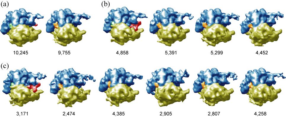
(a–c) Refined maps for MLF3D runs with 2, 4 and 6 references, respectively, and the number of particles contributing to each map. 50S ribosomal subunits are coloured blue, 30S subunits yellow, EF-G red, tRNA at the E site orange, and tRNA at the hybrid P/E site green. The results from the runs with 4 or 6 references were interpreted as successful classifications of ribosomes with or without EF-G. The separation in the run with 2 references is probably incomplete, as indicated by the weak density for EF-G.

MLF3D on large T-antigen data

Then, we applied MLF3D to a new cryo-EM data set of Simian Virus 40 large T-antigen (SV40 LTA) dodecamers in complex with an asymmetric double stranded DNA probe containing the origin of SV40 replication (Figure 2a). Preliminary 2D and 3D analyses of these data revealed a high degree of variability in the orientations of the central N-terminal domains with respect to the C-terminal regions (not shown). Therefore, we restricted our structural analysis to the more rigid C-terminal domains of this complex. Via preliminary 2D alignment and classification, we selected 3,859 side view projections of LTA dodecamers in complex with the dsDNA probe, and extracted sub-images of the two distal, C-terminal regions of each particle by windowing operations (Figure 2b). By processing these sub-images independently, we aimed to circumvent alignment and classification problems arising from the variable N-terminal domains. As the asymmetric DNA probe was designed to extend 23 base pairs (approximately 80 Å) from one side of the LTA dodecamer and 0 base pairs on the other side, the classification task for the 7,718 sub-images at hand consisted of separating the sub-images with the protruding DNA probe from their counterparts.

Figure 2. Application of MLF3D to large T-antigen C-terminal domains.

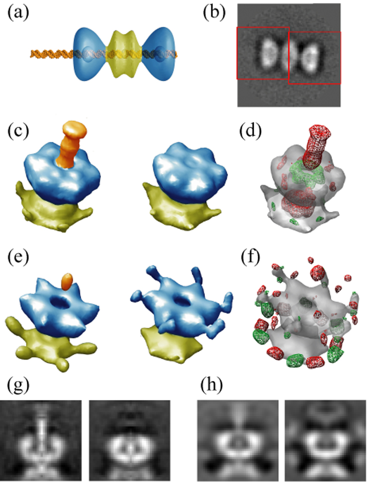
(a) Model representation for the complex between the LTA dodecamer and the asymmetric double stranded DNA probe. The C-terminal domains are coloured in blue, the N-terminal domains in yellow, and the DNA in orange. (b) Illustration of the windowing operations (40×40 pixels; red) based on a preliminary 2D alignment of the dodecamers. (c) Refined references as obtained with MLF3D, using the same colour code as in (a). (d) Difference map between the two references as obtained with MLF3D, with positive densities in red and negative differences in green, both contoured at three standard deviations of the difference map. (e–f) As in (c–d) but for the ML3D run. (g–h) Central slices through the maps shown in (c) and (e), respectively.

We performed an MLF3D classification with K=2, and compared the results with a similar ML3D run. A 56 Å low-pass filtered version of the crystal structure of the C-terminal domain (PDB-id: 1svl) was used as a starting model to generate the initial refinement seeds. The refined maps of the MLF3D were interpreted as a result of the expected classification, since the major difference between them resided in an approximately 75 Å long and 20 Å wide rod of density that was attributed to the overhanging DNA probe, and which extended well beyond three standard deviations of the difference map (Figure 2c–d,g). As opposed to these results, the refined maps obtained by ML3D classification were noisier and showed artefacts at the periphery of the C-terminal rings and in the form of low density regions at their centres (Figure 2e,h). Although some difference density due to the overhanging DNA could be observed, very little features extended beyond three standard deviations in the corresponding difference map (Figure 2f).

MLF2D on archaeal helicase MCM data

To assess the effectiveness of the MLF approach in 2D, we applied this algorithm to a cryo-EM data set comprising 4,042 top views of MCM from Methanobacterium thermoautotrophicum. This archaeal helicase was observed previously to assemble predominantly as 6 or 7-membered rings (Gómez-Llorente et al., 2005). Given that beforehand we did not know the number of distinct structures in the data, we performed independent classification runs with 3, 5 or 7 references, and compared the performance of the MLF2D algorithm with that of the ML2D approach (Scheres et al., 2005b) (Figure 3).

Figure 3. Application of MLF2D to MCM data.

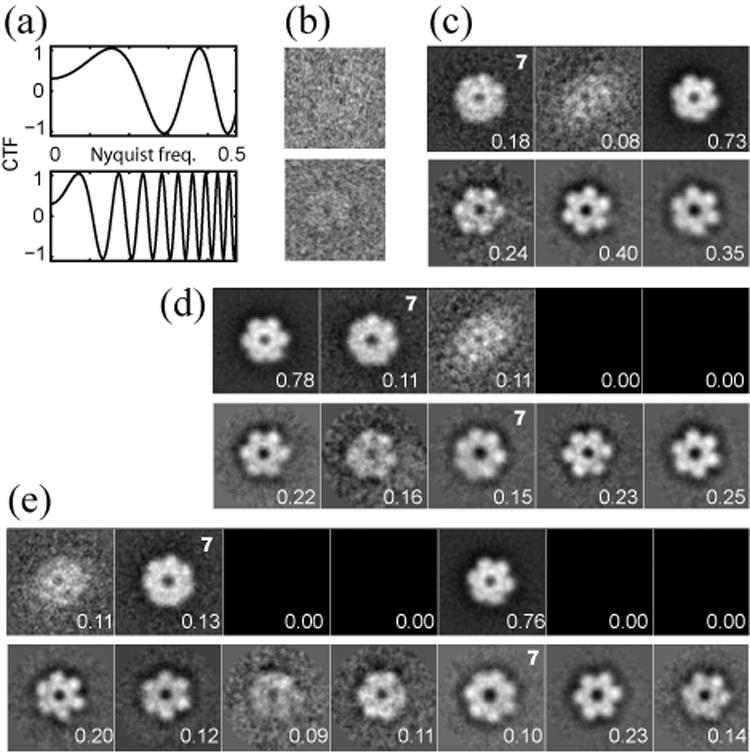
(a) Estimated CTF curves for the defocus groups with the smallest defocus value (−1.1 µm; top) and the largest defocus value (−5.1 µm; bottom). (b) Example images corresponding to the defocus groups as shown in (a). (c–e) Refined references for MLF2D (top rows) and ML2D (bottom rows) runs with 3, 5 and 7 references, respectively. The fraction of integrated probability weights for each class is indicated in the lower right corner of each reference. References that were interpreted as 7-fold symmetric particles are indicated with a 7 in the upper right corner.

The results of the three MLF2D runs with different number of references are highly consistent. In each run, one reference corresponded to a 6-membered ring, one reference to a 7-membered ring, and one reference to junk particles. Using more than three references resulted in additional “empty” classes, with zero contributing images. Moreover, hard classifications based on the maximum of the probability distributions indicate that the corresponding classes of 7-membered rings of the different runs overlapped up to 87%. Repetition of these runs starting from different random seeds showed very similar results (not shown).

The results of the ML2D classification approach show a different picture. In the calculation with 3 references, all 3 classes correspond to 6-membered rings. Classes corresponding to 7-membered rings are only observed when using 5 or 7 references, and these classes overlap to 83%. Furthermore, the number of particles contributing to each class tends to be more evenly distributed than in the MLF2D runs, and more of the class averages correspond to 6-membered rings with slightly different appearances. Further analysis of the particles assigned to these classes revealed that the classification resulted in a separation partially due to the occurrence of different defocus values in the images, despite the fact that the CTF phases had been corrected.

MLF2D on synthetic data

To investigate the potentials of the novel approach in more detail, we performed multiple MLF2D runs on synthetic data. For this purpose, we simulated structurally heterogeneous data sets by applying 1,500 random in-plane rotations and translations to each of two phantom images of 32×32 pixels, representing projections of a ring made of six or seven spheres, respectively. These phantoms were also used previously for the introduction of the white-noise ML2D approach (Scheres et al., 2005b). The in-plane rotations were distributed uniformly, the translations according to a 2D Gaussian centred at the image origin and with a standard deviation of 2 pixels. Data sets with different SNRs were created by adding increasing amounts of (white) Gaussian noise to the data. Subsequently, both the signal and the noise were affected by the simulated effects of an electron microscope. To this purpose, the 1,500 particles of each of the phantom images in every data set were divided in 3 subsets of 500 particles, each of which were filtered with one of 3 different CTFs (Figure 4a–b). The data sets thus obtained had quadratic SNRs (as defined in (Frank, 2006)) ranging from 0.02 to 0.25.

Figure 4. Application of MLF2D to synthetic test data.

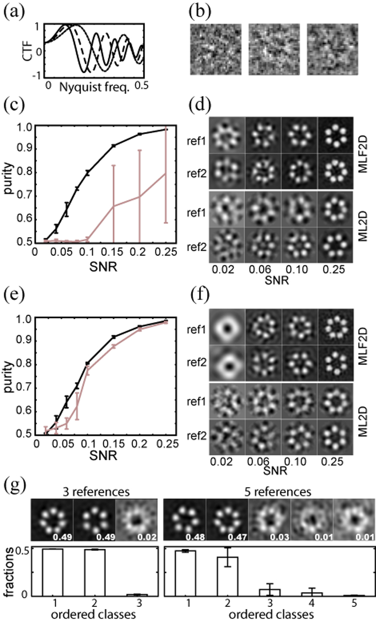
(a) The three CTFs that were applied to the test data, with defocus values of −1.5, −2.5 and −3.5 µm. (b) Examples of simulated images with a signal to noise ratio of 0.1 (one for each CTF). (c) Average and standard deviation for the class purities as obtained in five MLF2D (black) and five ML2D (grey) runs, using the complete set of 2×1,500 simulated particles with the three different CTFs at varying SNRs. The definition of class purity is as defined on p. 549 of (Tan et al., 2006). Note that purities range from 0.5 for random classifications to 1.0 for perfect classifications. (d) Corresponding refined references for the solution with the third best purity for MLF2D (top) and ML2D runs (bottom) with data at varying SNRs. (e) As (c), but only using the 2×500 simulated particles with the CTF as indicated with a dashed line in (a). (f) As (d), but for the runs presented in (e). (g) Bottom row: average and standard deviation for the relative class sizes (fraction of integrated probability weights), ordered from the largest to the smallest class for five independent runs with three (left) or five (right) references, using the data comprising all three CTFs and with a SNR of 0.15. Top row: the corresponding class averages for the run with the third highest sum of probability weights in two largest classes. The fraction of integrated probability weights for each class is indicated in the lower right corner of each reference.

We repeatedly applied MLF2D classification to each of these data sets and compared the results with those obtained using the ML2D approach (Figure 4c–d). For the entire range of SNR values tested, MLF2D yielded significantly better results, i.e. purer classes and cleaner reference images than ML2D. Even at relatively high SNRs, ML2D classification shows relatively low average class purities and with high standard deviations among the purities obtained in the independent runs. Further analysis showed that for these data, the ML2D approach sometimes correctly classified the structural heterogeneity, but other times it classified particles according to their defocus value. The MLF approach did not suffer from classification according to defocus value, and classified the structural heterogeneity even for data with SNRs as low as 0.06.

To eliminate the effects of classification by defocus values from our analyses, we repeated these calculations using only the subset of 1,000 images with a defocus of 2.5 µm (Figure 4e,f). In this case, for data with a SNR of 0.1 or higher both MLF2D and ML2D were capable of classifying the structural heterogeneity in each of the five runs performed. However, MLF2D still yielded purer classes and cleaner reference images than ML2D. Moreover, for data with SNRs lower than 0.1 ML2D failed, while MLF2D still classified the structural heterogeneity for data with SNRs in the range of 0.06–0.1.

Finally, to further investigate the behaviour of the novel approach with respect to the number of classes, we performed five independent classification runs using either 3 or 5 references for the simulated dataset with a SNR of 0.15 and comprising images with 3 different CTFs. As observed for the MCM data set, a strong tendency to converge to classes of highly unequal size was observed. In particular, the two major classes of all runs corresponded to the two different phantom structures in the simulated data, and very few particles contributed to the remaining number of classes (Figure 4g).

Discussion

Given the abundant levels of experimental noise in cryo-EM data, approaches with a statistical noise model are expected to provide suitable solutions for the image processing problems in this field. In particular structurally heterogeneous data, containing projections of macromolecular machines in distinct structural states, have posed serious limitations on the applicability of 3D-EM techniques. Therefore, it is interesting to see the growing number of Expectation-Maximization approaches for cryo-EM image alignment, reconstruction and classification tasks. The robustness of these approaches has been illustrated on several occasions, and their effectiveness is also illustrated by their use in an increasing number of cryo-EM laboratories (e.g. see (Dang et al., 2005; Gubellini et al., 2006; Martín-Benito et al., 2007; Schleiff et al., 2003; Stirling et al., 2006)). Still, the statistical data model adopted in these approaches is known to be apt for improvement, as CTF effects are ignored and the assumption of uncorrelated (i.e. white) noise is known to be a poor one for 3D-EM data. In the work presented here, we propose a more realistic data model for cryo-EM images and present the corresponding Expectation-Maximization like algorithms for 2D and 3D alignment and classification of structurally heterogeneous projection data.

The probability distributions of the proposed statistical model are expressed in Fourier space. In this way, we model spatially stationary (i.e. non-white) noise by using Gaussian distributions with varying widths at different spatial frequencies. As the power of the experimental noise in cryo-EM data typically also varies with spatial frequency, the proposed model is probably more accurate than a white noise model. The assumption of white noise in conventional approaches is a consequence of assuming independence between the probability distributions of all (real-space) pixels of an image. In the MLF approach, this assumption has been traded for the assumption of independence between the probability distributions of all Fourier components. This assumption is probably a more reasonable one, as long as the images are not masked in real-space. Multiplication with a mask in real-space is equivalent to a convolution with the transform of the window function in Fourier-space, which introduces correlations in the noise in Fourier-space. Therefore, perhaps in contrary to general practice in 3D-EM, we do not mask our experimental images when applying this approach. In this respect, the presence of closely neighbouring particles may present a problem for some data sets, and this will be a subject of future research.

The proposed algorithms employ a Wiener filter to deconvolve the CTF-affected images. In addition, we implemented an automated multi-resolution approach, where the number of Fourier pixels included is gradually increased throughout the refinement process, as the quality of the estimated model parameters improves. In a strict sense, these modifications deviate from the Expectation-Maximization regime, meaning that our algorithms do not explicitly maximize a log-likelihood target function. The maximum-likelihood solution to CTF restoration is a pseudo-inverse filter, which is known to work poorly in the presence of noise in the data (Trussel, 1984). Furthermore, as the model typically contains only low-frequency information at the early stages of refinement, limiting the probability calculations to those frequencies may not only lead to increased robustness and radius of convergence (cf. (Dengler, 1989; Doerschuk and Johnson, 2000; Sorzano et al., 2004a; Stewart and Grigorieff, 2004)), but also to a computationally more efficient algorithm. Therefore, we consider our implementation of the adaptive Wiener filter and the multi-resolution approach in the MLF algorithms as necessary or at least practical modifications of the theoretical Expectation-Maximization algorithms. However, this also means that the convergence behaviour of the MLF algorithms is no longer guaranteed by mathematical theorems. Therefore, we empirically validated that the log-likelihood indeed increases at every iteration for representatives of all runs presented in this paper (see Supplemental Figure 2). The fact that this was the case for almost all calculations suggests that our deviations from the strict Expectation-Maximization regime are reasonable at least. In addition, we compared our results with those obtained using a strict (Generalized) Expectation-Maximization algorithm, with a CTF pseudo-inverse pre-filtering of the data and limiting all calculations to those frequencies before the one where the CTF with the highest defocus value passes through zero (see Supplemental Figure 3). The strict GEM algorithms converge to comparable solutions as those obtained with the MLF algorithms, separating the data into similar classes as those presented in the Results section. The somewhat improved performance of the MLF algorithms may be considered as a validation of the modifications exposed above.

An important effect of CTF correction is that it prevents the novel algorithms from classification of particles according to their defocus value, as was sometimes observed for the white noise approach. Since separation according to defocus value competes with the separation of structural variability, it may severely affect the classification results. Consequently, MLF2D performed significantly better than ML2D in our tests on synthetic data, even at relatively high signal to noise ratios (Figure 4c–d). Similarly, the use of three references in the ML2D classification of MCM particles resulted in three structurally similar classes, but with distinct average defocus values (Figure 3c). Two ways could be proposed to circumvent the problem of classifying particles according to their defocus value. Firstly, the inclusion of more references in the refinement could be used to allow both separation of structural variability and separation according to defocus value. This approach was applied successfully to the 2D averaging of the MCM data (Figure 3d–e). Secondly, one may opt to process the data in so-called defocus groups, where particles with similar defocus values are processed independently. The efficiency of this approach was illustrated for the 2D averaging of the synthetic data (Figure 4e–f). In practice however, the number of available experimental images is often too small to apply any of these two solutions. This is particularly the case for the 3D problem, where a large number of images need to be combined in each 3D reconstruction, and where apart from structural variability and distinct defocus values, a third effect competes in the particle classification. Due to computational limitations, the angular sampling in the current implementations of both MLF3D and ML3D is typically limited. This may result in the convergence towards slightly rotated, but otherwise structurally identical references (Figure 1b–c), apparently to accommodate particles with projection directions falling in between the angular grid used (cf. (Scheres et al., 2007)). Consequently, the ML3D approach would require a higher number of references than the expected number of structural states to compensate both for the limited angular sampling and for the separation by defocus value. As the MLF approach does not suffer from classification according to defocus value, this approach allows combination of all particles in a single optimization process, which is a considerable advantage.

A second advantage that may be related with CTF correction is illustrated by application of MLF3D to the sub-images of the C-terminal regions of large T-antigen in complex with a DNA probe containing the origin of SV40 replication. Since LTA dodecamers do not assemble in the absence of DNA, and because of the asymmetric design of the DNA probe, we know that dsDNA should protrude from one side of the complex. Still, in our experience its visualization poses a challenge to alignment and classification algorithms. This is also illustrated by the average image in Figure 2b that lacks DNA density, probably as a result of a mediocre alignment caused by the large degree of structural variability in the data. Thus far, DNA density in 2D averages has only been observed using ML2D classification (Scheres et al., 2005b). In the 3D case, using either conventional angular refinement schemes (Valle et al., 2006), or the ML3D approach (Scheres et al., 2007), we were never capable of visualizing DNA density. Also for the data presented in this paper, the ML3D approach yielded reconstructions lacking DNA density, and consequently failed in classifying the particles from either side of the dodecamers (Figure 2d). Therefore it is remarkable that the MLF approach was capable of both visualizing the DNA in 3D and separating the particles with DNA from their counterparts without overhanging DNA (Figure 2c). Indeed, the dimensions of the density attributed to the DNA maps agreed well with the expected size of the overhanging DNA probe. We hypothesize that the CTF correction in the MLF approach may be responsible for this improvement. As a consequence of CTF correction, the aspect of the refined models (in 2D and in 3D) changes with respect to the conventional approach. The typical regions with negative density around the refined particles in the white noise approach are no longer observed with the new method. These regions are typically visible as black “halos” around white particles on a grey background (e.g. see Figure 2h). These effects, which are caused by the CTF, may interfere with the correct alignment of the relatively thin DNA as it sticks out of the LTA dodecamers into the negative density of the halo. For the CTF corrected references in the MLF algorithms, these black halos no longer exist (the references are typically observed as white particles on a black background; see Figure 2g), so that they no longer interfere with the correct alignment of the DNA.

The application of MLF2D to the experimental MCM data set revealed another interesting type of behaviour of the novel algorithm (Figure 3). The number of references to use in the optimization process is the most important free parameter in both the MLF and the conventional ML classification approaches. This number ideally should reflect the number of distinct structural states in the data, which unfortunately is not known a priori under typical experimental conditions. However, irrespective of the number of references used for the MCM data, the new approach converged to three structurally distinct references, and the remaining references converged to empty classes, i.e. without any contributing particles. This tendency to converge to (almost) empty classes when using a higher number of references than the number of distinct structures in the data, was also confirmed by application to simulated data (Figure 4g). Possibly, this desirable behaviour is a consequence of the more realistic data model, describing the experiment in a more adequate way. In any case, as the optimal choice for the number of classes is a key issue in pattern recognition (Young and Fu, 1986), the fact that the new algorithm seems to partially overcome this problem (at least in 2D) by the stability of the results for a range of class numbers, opens a range of interesting new possibilities that will be the subject of future research.

Based on the observations presented above, we conclude that the proposed model for cryo-EM data and the corresponding Expectation-Maximization like algorithms for alignment and classification provide notable advantages over existing approaches. In particular, the spatial frequency-dependent description of the noise, the ability to combine images with distinct defocus values in a single optimization process and the correction of CTF effects on the references are marked improvements. The presented algorithms have been implemented in the open-source package Xmipp (Sorzano et al., 2004b) and are generally applicable to structurally heterogeneous cryo-EM data. As such, the proposed approach may represent a significant contribution to the development of cryo-EM image processing tools that allow visualization of distinct structural states for a wide range of macromolecular machines.

Experimental procedures

Implementation

The algorithms for 2D and 3D MLF classification were implemented in the open-source package Xmipp (Sorzano et al., 2004b). The discretization of the rotational angles, parallelization through a message-passing interface (MPI), the convergence criteria, the modelling of 3D objects by blobs (Marabini et al., 1998), and the 3D reconstructions by the modified weighted-least squares ART algorithm are all as described for the corresponding white noise approaches (Scheres et al., 2007; Scheres et al., 2005b). With respect to the integrations over all translations, some changes were made. Calculation of the probability-weighted averages for the updates of the model parameters entails exhaustive integrations over all classes, in-plane rotations and translations. In the white-noise approach, all translations for a given class and in-plane rotation could be calculated in an efficient way using fast Fourier transforms. By expressing the probabilities in Fourier space this is no longer possible, and all translations need to be evaluated one at a time (through phase shifts of the Fourier components), which strongly affects the computational efficiency of the algorithms. Therefore, besides reducing the vast search space as presented previously (Scheres et al., 2005a), we limited all translational searches to a user-provided range around the optimal translations from the previous iteration (i.e. we implicitly assume a zero-valued pdf outside the search range). For all calculations presented in this work, we used a range of +/−3 pixels in both directions. Thereby, the computational costs of the MLF2D and MLF3D algorithms were observed to be comparable to those of the ML2D and ML3D algorithms (results not shown).

Refinement protocols

All MLF2D and ML2D runs were performed until convergence as defined previously (Scheres et al., 2005b), using a 5° sampling for the in-plane rotations. The MLF3D and ML3D runs comprised 20 iterations for the ribosome data, and 25 iterations for the LTA data, and all corresponding 3D reconstructions were performed using the default parameters of the wlsART algorithm (λ=0.2, κ=0.5 and M=10). For the ribosome refinements, exhaustive integrations over all orientations were performed, using an angular sampling of 12°. All LTA refinements were performed using an angular sampling of 10° and imposing 6-fold symmetry. In addition, to reflect the prior knowledge that all images were side view projections of the dodecameric complexes, the tilt-angle integrations were limited to 50–130 degrees (again assuming zero-valued pdfs outside this range). To prevent the inclusion of high-frequency terms too early in the MLF refinements, all estimated spectral SNRs in the MLF3D runs for the LTA data and the MLF2D runs for the simulated data were multiplied by 0.25.

Ribosome data

The employed data on 70S E.coli ribosomes is a subset of 20,000 randomly selected images of a cryo-EM data set that was presented previously (Scheres et al., 2007). These data comprised normalized, CTF-phase corrected, and down-scaled images of 64×64 pixels (with a pixel size of 5.6 Å). For the MLF3D approach, the data were divided in 9 distinct defocus groups, with average defocus values ranging from −1.1 µm to −3.8 µm.

Large T-antigen data

Simian Virus 40 LTA was purified as reported previously (Simanis and Lane, 1985). The asymmetric double stranded DNA probe comprising the origin of SV40 replication was obtained by PCR using primers oligo-EcoRI (5’-GAA-TTC-CCG-GGG-ATC-CGG-TCG-AC-3’) and oligo-HindIII (5’-AAG-CTT-TCT-CAC-TAC-TTC-TGG-AAT-AGC-3’) and plasmid pOR1 as a template (DeLucia et al., 1986). This 107 base pair long probe was designed to extend 23 base pairs at the AT-rich region binding side of the LTA dodecamers. Complexes of LTA dodecamers and DNA were prepared as described previously (Valle et al., 2006). The sample was vitrified on glow-discharged Quantifoil grids, and micrographs were recorded under low-dose conditions at a magnification of 50,000× on a FEI Tecnai F20 with a field emission gun, operated at 200 kV. The micrographs were scanned on a Zeiss Photoscan TD scanner with a pixel size corresponding to 2.8 Å. Down-sampling by linear interpolation yielded a final pixel size of 5.6 Å. For each micrograph, the CTF was estimated using CTFFIND (Mindell and Grigorieff, 2003) and the phases of the Fourier components were corrected using a standard phase flipping protocol. Side view projections of the LTA dodecamers were manually selected, extracted as images of 80×80 pixels and normalized. Subsequently, from each side view projection, two sub-images of 40×40 pixels were extracted as described in the main text. For the MLF3D approach, the data were divided in 7 defocus groups, with average defocus values ranging from −3.8 µm to −6.8 µm.

MCM data

Methanobacterium thermoautotrophicum MCM was purified as described previously (Gómez-Llorente et al., 2005). Protein samples were vitrified and imaged as described for the LTA data. Micrographs were digitized in a Zeiss Photoscan TD scanner with a pixel size corresponding to 1.4 Å, and down-sampled to a final pixel size of 4.2 Å. The CTF parameters for each micrograph were estimated, and the corresponding phases were corrected as described for the LTA data. Top views of MCM complexes were selected manually, extracted as 64×64 pixel images, and normalized. For the MLF2D runs, the data were divided into 7 defocus groups with average defocus values ranging from −1.1 to −5.1µm.

References

- Adams PD, Pannu NS, Read RJ, Brunger AT. Cross-validated maximum likelihood enhances crystallographic simulated annealing refinement. Proc Natl Acad Sci U S A. 1997;94:5018–5023. doi: 10.1073/pnas.94.10.5018. [DOI] [PMC free article] [PubMed] [Google Scholar]
- Carazo JM, Rivera FF, Zapata EL, Radermacher M, Frank J. Fuzzy sets-based classification of electron microscopy images of biological macromolecules with an application to ribosomal particles. J Microsc. 1990;157:187–203. doi: 10.1111/j.1365-2818.1990.tb02958.x. [DOI] [PubMed] [Google Scholar]
- Dang TX, Hotze EM, Rouiller I, Tweten RK, Wilson-Kubalek EM. Prepore to pore transition of a cholesterol-dependent cytolysin visualized by electron microscopy. J Struct Biol. 2005;150:100–108. doi: 10.1016/j.jsb.2005.02.003. [DOI] [PubMed] [Google Scholar]
- DeLucia AL, Deb S, Partin K, Tegtmeyer P. Functional interactions of the simian virus 40 core origin of replication with flanking regulatory sequences. J Virol. 1986;57:138–144. doi: 10.1128/jvi.57.1.138-144.1986. [DOI] [PMC free article] [PubMed] [Google Scholar]
- Dempster AP, Laird NM, Rubin DB. Maximum-likelihood from incomplete data via the EM algorithm. J Royal Statist Soc Ser B. 1977;39:1–38. [Google Scholar]
- Dengler J. A multi-resolution approach to the 3D reconstruction from an electron microscope tilt series solving the alignment problem without gold particles. Ultramicroscopy. 1989;30:337–348. [Google Scholar]
- Doerschuk PC, Johnson JE. Ab initio reconstruction and experimental design for cryo electron microscopy. IEEE Transactions on Information Theory. 2000;46:1714–1729. [Google Scholar]
- Frank J. Three-dimensional Electron Microscopy of Macromolecular Assemblies. New York: Oxford University Press; 2006. [Google Scholar]
- Gómez-Llorente Y, Fletcher RJ, Chen XS, Carazo JM, San Martín C. Polymorphism and double hexamer structure in the archaeal minichromosome maintenance (MCM) helicase from Methanobacterium thermoautotrophicum. J Biol Chem. 2005;280:40909–40915. doi: 10.1074/jbc.M509760200. [DOI] [PubMed] [Google Scholar]
- Grigorieff N. FREALIGN: high-resolution refinement of single particle structures. J Struct Biol. 2007;157:117–125. doi: 10.1016/j.jsb.2006.05.004. [DOI] [PubMed] [Google Scholar]
- Gubellini F, Francia F, Busselez J, Venturoli G, Levy D. Functional and structural analysis of the photosynthetic apparatus of Rhodobacter veldkampii. Biochemistry. 2006;45:10512–10520. doi: 10.1021/bi0610000. [DOI] [PubMed] [Google Scholar]
- Lehmann EL, Casella G. Theory of Point Estimation. 2nd edition edn. New York: Springer-Verlag; 1998. [Google Scholar]
- Leschziner AE, Nogales E. Visualizing Flexibility at Molecular Resolution: Analysis of Heterogeneity in Single-Particle Electron Microscopy Reconstructions. Annu Rev Biophys Biomol Struct. 2007;36:43–62. doi: 10.1146/annurev.biophys.36.040306.132742. [DOI] [PubMed] [Google Scholar]
- Llorca O. Introduction to 3D reconstruction of macromolecules using single particle electron microscopy. Acta Pharmacol Sin. 2005;26:1153–1164. doi: 10.1111/j.1745-7254.2005.00203.x. [DOI] [PubMed] [Google Scholar]
- Marabini R, Herman GT, Carazo JM. 3D reconstruction in electron microscopy using ART with smooth spherically symmetric volume elements (blobs) Ultramicroscopy. 1998;72:53–65. doi: 10.1016/s0304-3991(97)00127-7. [DOI] [PubMed] [Google Scholar]
- Martín-Benito J, Gómez-Reino J, Stirling PC, Lundin VF, Gómez-Puertas P, Boskovic J, Chacón P, Fernández JJ, Berenguer J, Leroux MR, Valpuesta JM. Divergent substrate-binding mechanisms reveal an evolutionary specialization of eukaryotic prefoldin compared to its archaeal counterpart. Structure. 2007;15:101–110. doi: 10.1016/j.str.2006.11.006. [DOI] [PubMed] [Google Scholar]
- Mindell JA, Grigorieff N. Accurate determination of local defocus and specimen tilt in electron microscopy. J Struct Biol. 2003;142:334–347. doi: 10.1016/s1047-8477(03)00069-8. [DOI] [PubMed] [Google Scholar]
- Pascual A, Bárcena M, Merelo JJ, Carazo JM. Mapping and fuzzy classification of macromolecular images using self-organizing neural networks. Ultramicroscopy. 2000;84:85–99. doi: 10.1016/s0304-3991(00)00022-x. [DOI] [PubMed] [Google Scholar]
- Pascual-Montano A, Donate LE, Valle M, Bárcena M, Pascual-Marquí RD, Carazo JM. A novel neural network technique for analysis and classification of EM single-particle images. J Struct Biol. 2001;133:233–245. doi: 10.1006/jsbi.2001.4369. [DOI] [PubMed] [Google Scholar]
- Penczek P, Zhu J, Schroeder R, Frank J. Three dimensional reconstruction with contrast transfer compensation from defocus series. Scanning Microscopy. 1997;11:147–154. [Google Scholar]
- Provencher SW, Vogel RH. Three-dimensional reconstruction from electron micrographs of disordered specimens. I. Method. Ultramicroscopy. 1988;25:209–221. doi: 10.1016/0304-3991(88)90016-2. [DOI] [PubMed] [Google Scholar]
- Read RJ. Pushing the boundaries of molecular replacement with maximum likelihood. Acta Crystallogr D Biol Crystallogr. 2001;57:1373–1382. doi: 10.1107/s0907444901012471. [DOI] [PubMed] [Google Scholar]
- Scheres SHW, Gao H, Valle M, Herman GT, Eggermont PP, Frank J, Carazo JM. Disentangling conformational states of macromolecules in 3D-EM through likelihood optimization. Nat Methods. 2007;4:27–29. doi: 10.1038/nmeth992. [DOI] [PubMed] [Google Scholar]
- Scheres SHW, Valle M, Carazo JM. Fast maximum-likelihood refinement of electron microscopy images. Bioinformatics. 2005a;21 Suppl 2:ii243–ii244. doi: 10.1093/bioinformatics/bti1140. [DOI] [PubMed] [Google Scholar]
- Scheres SHW, Valle M, Núñez R, Sorzano COS, Marabini R, Herman GT, Carazo JM. Maximum-likelihood multi-reference refinement for electron microscopy images. J Mol Biol. 2005b;348:139–149. doi: 10.1016/j.jmb.2005.02.031. [DOI] [PubMed] [Google Scholar]
- Schleiff E, Soll J, Kuchler M, Kuhlbrandt W, Harrer R. Characterization of the translocon of the outer envelope of chloroplasts. J Cell Biol. 2003;160:541–551. doi: 10.1083/jcb.200210060. [DOI] [PMC free article] [PubMed] [Google Scholar]
- Sigworth FJ. A maximum-likelihood approach to single-particle image refinement. J Struct Biol. 1998;122:328–339. doi: 10.1006/jsbi.1998.4014. [DOI] [PubMed] [Google Scholar]
- Simanis V, Lane DP. An immunoaffinity purification procedure for SV40 large T antigen. Virology. 1985;144:88–100. doi: 10.1016/0042-6822(85)90308-3. [DOI] [PubMed] [Google Scholar]
- Sorzano COS, Jonic S, El-Bez C, Carazo JM, De Carlo S, Thevenaz P, Unser M. A multiresolution approach to orientation assignment in 3D electron microscopy of single particles. J Struct Biol. 2004a;146:381–392. doi: 10.1016/j.jsb.2004.01.006. [DOI] [PubMed] [Google Scholar]
- Sorzano COS, Marabini R, Velázquez-Muriel J, Bilbao-Castro JR, Scheres SHW, Carazo JM, Pascual-Montano A. XMIPP: a new generation of an open-source image processing package for electron microscopy. J Struct Biol. 2004b;148:194–204. doi: 10.1016/j.jsb.2004.06.006. [DOI] [PubMed] [Google Scholar]
- Stewart A, Grigorieff N. Noise bias in the refinement of structures derived from single particles. Ultramicroscopy. 2004;102:67–84. doi: 10.1016/j.ultramic.2004.08.008. [DOI] [PubMed] [Google Scholar]
- Stirling PC, Cuellar J, Alfaro GA, El Khadali F, Beh CT, Valpuesta JM, Melki R, Leroux MR. PhLP3 modulates CCT-mediated actin and tubulin folding via ternary complexes with substrates. J Biol Chem. 2006;281:7012–7021. doi: 10.1074/jbc.M513235200. [DOI] [PubMed] [Google Scholar]
- Tan PN, Steinbach M, Kumar V. Introduction to data mining. Addison-Wesley; 2006. [Google Scholar]
- Terwilliger TC. Maximum-likelihood density modification. Acta Crystallogr D Biol Crystallogr. 2000;56:965–972. doi: 10.1107/S0907444900005072. [DOI] [PMC free article] [PubMed] [Google Scholar]
- Trussel HJ. A priori knowledge in algebraic reconstruction methods. In: Huang TS, editor. Image reconstruction in incomplete observations. London: Jai Press; 1984. [Google Scholar]
- Unser M, Sorzano COS, Thevenaz P, Jonic S, El-Bez C, De Carlo S, Conway JF, Trus BL. Spectral signal-to-noise ratio and resolution assessment of 3D reconstructions. J Struct Biol. 2005;149:243–255. doi: 10.1016/j.jsb.2004.10.011. [DOI] [PMC free article] [PubMed] [Google Scholar]
- Unser M, Trus BL, Steven AC. A new resolution criterion based on spectral signal-to-noise ratios. Ultramicroscopy. 1987;23:39–51. doi: 10.1016/0304-3991(87)90225-7. [DOI] [PubMed] [Google Scholar]
- Valle M, Chen XS, Donate LE, Fanning E, Carazo JM. Structural basis for the cooperative assembly of large T antigen on the origin of replication. J Mol Biol. 2006;357:1295–1305. doi: 10.1016/j.jmb.2006.01.021. [DOI] [PubMed] [Google Scholar]
- Yin Z, Zheng Y, Doerschuk PC, Natarajan P, Johnson JE. A statistical approach to computer processing of cryo-electron microscope images: virion classification and 3-D reconstruction. J Struct Biol. 2003;144:24–50. doi: 10.1016/j.jsb.2003.09.023. [DOI] [PubMed] [Google Scholar]
- Young TY, Fu K-S. Handbook of pattern recognition and image processing. San Diego: Academic Press; 1986. [Google Scholar]
Associated Data
This section collects any data citations, data availability statements, or supplementary materials included in this article.