Linkage Disequilibrium Under Skewed Offspring Distribution Among Individuals in a Population

Abstract

Correlations in coalescence times between two loci are derived under selectively neutral population models in which the offspring of an individual can number on the order of the population size. The correlations depend on the rates of recombination and random drift and are shown to be functions of the parameters controlling the size and frequency of these large reproduction events. Since a prediction of linkage disequilibrium can be written in terms of correlations in coalescence times, it follows that the prediction of linkage disequilibrium is a function not only of the rate of recombination but also of the reproduction parameters. Low linkage disequilibrium is predicted if the offspring of a single individual frequently replace almost the entire population. However, high linkage disequilibrium can be predicted if the offspring of a single individual replace an intermediate fraction of the population. In some cases the model reproduces the standard Wright–Fisher predictions. Contrary to common intuition, high linkage disequilibrium can be predicted despite frequent recombination, and low linkage disequilibrium under infrequent recombination. Simulations support the analytical results but show that the variance of linkage disequilibrium is very large.

LINKAGE disequilibrium (LD) refers to the nonrandom association of alleles at different loci (Lewontin and Kojima 1960). Changes in population size, natural selection, population structure, and random drift can all lead to LD. Recombination, or the reciprocal exchange of material between homologous chromosomes, breaks down associations between alleles at different loci. Estimating LD can thus give insight into the forces that have shaped extant genetic diversity. The potential utility of LD for fine-scale mapping of human disease loci has also raised interest in estimating levels of linkage disequilibrium in human populations (Jorde 1995; Lander 1996; Risch and Merikangas 1996). The evolutionary history of many organisms is marked by growth and decline of populations as well as various kinds of subdivision (with or without migration and admixture). As an example, the Icelandic human population has undergone severe bottlenecks, accompanied by recent population growth, in its ∼1100-year history (Thorarinsson 1961; Thorsteinsson and Jónsson 1991; Jónsson and Magnússon 1997). Bataillon et al. (2006) report extensive linkage disequilibrium in the Icelandic human population and estimate the effective population size N_e to be ∼5000, much less than the current census size of ∼300,000 (Garđarsdóttir and Sigurjónsson 2006).

Linkage disequilibrium is a function of the frequencies of alleles in the population and LD can be quantified as a function of allele frequencies in a number of ways (cf. Hedrick 2000). One commonly used measure of LD is the coefficient D of linkage disequilibrium and is defined as the difference between the observed frequency of a gametic type (haplotype) and the frequency expected on the basis of random association of alleles in gametes (Lewontin and Kojima 1960). The coefficient D can be written as D = P_ABP_ab – P_aBP_Ab in which P_xy is the frequency of haplotype xy. High absolute values of D correspond to high linkage disequilibrium in the population.

Following Slatkin (1994) we can understand the effects of population history on LD between two diallelic loci by considering the shape of the gene genealogy of a sample without recombination. In this case the alleles at both loci have the same gene genealogy. As an example, consider a population that has recently grown in size. Figure 1a shows a gene genealogy of a sample from a population that has experienced recent expansion. A single neutral mutation has arisen at each locus. The location of the mutations on the gene genealogy determines the level of linkage disequilibrium. Since neutral mutations arise randomly on the genealogy, the shape of the gene genealogy becomes a deciding factor. A gene genealogy of a sample from a recently expanded population is composed mainly of external branches. This happens because most coalescence events occur in the smaller ancestral population. Hence, each mutation is most likely to arise on an external branch and will therefore be present on a single haplotype in the sample. Thus the haplotypes observed in a sample of size n would be one each of aB and Ab, and n – 2 of AB. In this case, |D| = |((n – 2)/n) × 0 – 1/n²| = 1/n², which becomes quite small for large n.

Figure 1.—

Gene genealogies of a sample of two completely linked loci (a) from a population that has recently grown in size and (b) from a stable population. One mutation event is assumed at each locus, and the ancestral gametic type is AB. The sample in a consists of one each of aB and Ab, and four AB, indicating low linkage disequilibrium. The sample in b consists of the gametic types aB and Ab in equal proportions, indicating high linkage disequilibrium.

For comparison, Figure 1b shows a gene genealogy for a sample from a stable population. Now, the two mutations are more likely to co-occur on an internal branch that has, by definition, more than one descendent in the sample. The result is only two gametic types; i.e., we could observe n/2 each of aB and Ab, and it follows that D = , or the largest possible value that D can have. Any ancestral process that increases the chance of events like this will tend to increase LD.

In this work, we consider another commonly used measure of LD, r², which is given by

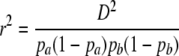(1)

(Hill and Robertson 1968), in which p_x is the frequency of allele x, and which is commonly used to estimate the statistical association between alleles at two loci. Ohta and Kimura (1971) suggested approximating the expected value of r² as a ratio of expected values. This approximation appears good provided the allele frequencies are not too small (Hudson 1985; McVean 2002). Considering the gene genealogy of a sample of size two from two loci and using the results of Strobeck and Morgan (1978) and Hudson (1985), McVean (2002) showed that an approximation to the expected value of r² can be written in terms of correlation in coalescence times. Griffiths (1981, 1991) (see also Pluzhnikov and Donnelly 1996; Durrett 2002) gives the covariances in coalescence times based on the standard Wright–Fisher model of reproduction (Fisher 1930; Wright 1931). Since McVean's (2002) approach makes no assumptions about reproduction, predictions about LD can be obtained under different population models.

The present study derives correlations in coalescence times in cases where a single individual can have very large number of offspring with some probability. In terms of reproduction, our model is a special case of the models considered by Sagitov (1999) and Pitman (1999). In terms of genetics, our model is novel because we include the possibility of recombination. Sagitov (1999) and Pitman (1999) did not consider recombination, but proved convergence to an ancestral process that allows for many ancestral lines to reach a common ancestor, or coalesce, at exactly the same instant (or same generation) and that occurs on a shorter timescale than in the standard coalescent (Pitman 1999; Sagitov 1999; Schweinsberg 2000; Möhle and Sagitov 2001). Predictions of patterns of genetic diversity also differ from those under Kingman's coalescent (Eldon and Wakeley 2006; Möhle 2006). Such models may be appropriate for many marine organisms with high fecundities and high mortality in early life stages or type III survivorship curves (Hedgecock 1994).

Depending on parameter values, these models can predict much lower levels of genetic variation than would be expected on the basis of census size. This is often observed in marine species and is quantified using the ratio of effective to census size, N_e/N. Low N_e/N ratios reported in Atlantic cod (Gadus morhua; Árnason 2004), red drum (Sciaenops ocellatus; Turner et al. 2002), and the Pacific oyster (Crassostrea gigas; Hedgecock 1994) have been thought to indicate high variance in offspring number (Crow and Kimura 1970; Hedrick 2005). Hedgecock (1994) proposed a “sweepstakes” reproduction model in which lucky individuals may contribute a large number of offspring to the next generation.

Here we show that allowing individuals to have many offspring typically results in low predicted LD in the population. In some cases, however, higher LD than that predicted under the standard Wright–Fisher model is obtained. Low LD can also be predicted under low recombination, and high LD under high recombination, contrary to common intuition. Finally, the different formulas representing different timescales on which recombination and random drift occur can predict the same level of linkage disequilibrium. This implies that it may be difficult to distinguish between the recombination parameter and the parameters controlling the size and frequency of the large reproduction events using sequence data. Our analytical results are for the expected value of r², but we have also performed a simulation study that shows that the variance of r² is typically very large.

THEORY AND METHODS

Population models:

The modified population model considered is a special case of the neutral population models analyzed by Sagitov (1999) and Pitman (1999). A discrete-generation model, it is a modification of the well-known Wright–Fisher (Fisher 1930; Wright 1931) model of reproduction. A modified Moran model (Moran 1958, 1962) of overlapping generations introduced and studied by Eldon and Wakeley (2006) was also considered. Since the results obtained under the modified Moran model (not shown) are compatible with those obtained under the modified Wright–Fisher population model, we consider only the modified Wright–Fisher model and results derived under that model from now on.

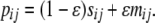
Eldon and Wakeley (2006) treated only haploid individuals. Since the present study addresses recombination, a diploid population is assumed. For the moment, consider a diploid population without recombination or mutation. Note that we do not treat mutation explicitly here, but follow McVean (2002) in assuming that the mutation rate per site is small. As usual, N denotes the population size. The Wright–Fisher model is modified as follows. With probability 1 – ɛ (0 < ɛ < 1) the usual Wright–Fisher sampling occurs; i.e., all individuals contribute equally to the next generation via multinomial sampling, and all are replaced by offspring each generation. With probability ɛ the offspring of a single randomly chosen individual replace a fraction ω of the population, and the other 2N – 1 individuals share the remaining 1 – ω fraction of reproduction events according to the usual Wright–Fisher sampling. The probability ɛ of modified Wright–Fisher sampling is taken as ɛ = φN ^−α in which both constants φ and α > 0. In Eldon and Wakeley (2006) φ = 1. The parameter φ allows us to adjust the relative rates of coalescence and recombination when both occur on the same timescale.

Our first concern is with the timescale of coalescence under this model. Under the modified Wright–Fisher population model the expected coalescence time of two lines can be much shorter than under the standard coalescent (Table 1). Consider first the case 0 < α < 1, in which α controls the timescale at which modified sampling occurs (ɛ = φ/N^α). In this case, the result is a multiple-mergers coalescent, since “ω-events” (a single individual has 2Nω offspring) occur on a shorter timescale (proportional to N^α generations) than the standard coalescent (timescale: proportional to N generations). In the case α = 1, all the coalescence events occur on the same timescale. When α > 1, the ω-events occur on a longer timescale than the standard coalescent and are thus negligible in large populations. In the first two cases (i.e., 0 < α ≤ 1), the expected time to coalescence is a function of φ and ω.

TABLE 1.

Expected time to coalescence of two lines under the modified Wright–Fisher population model

Case	λcoal	Timescale
0 < α < 1	φω2	Nα
α = 1	1 + φω2	2N
α > 1	1	2N

The rate of coalescence is denoted by λ_coal.

The term “x-merger” denotes the event that x ancestral lines derive from a single individual in one time step. Given n ancestral lines, we are interested in coalescent events: 2 ≤ x ≤ n. Let G_n,x denote the probability of an x-merger among n ancestral lines. In general, for finite N,

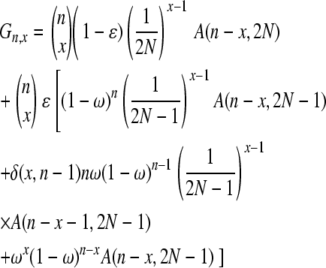(2)

in which A(m, M) = (1 – 1/M)(1 – 2/M) · · · (1 – m/M), A(0, M) = 1, and δ(·, ·) is the delta function

(3)

The function G_n,x determines the distribution of the size and shape of gene genealogies when there is no recombination.

McVean (2002) obtains an expression for an approximation to the expected value of r² in terms of covariances in coalescence times, assuming that the per-site mutation rate at each locus is very small. In so doing, the gene genealogy of a sample of size two at each of two loci is modeled backward in time using a Markov chain. There are three states in the chain, which correspond to three possible configurations of the sample, and are denoted 𝒮₀, 𝒮₁, and 𝒮₂ (see Figure 2). The subscripts 0, 1, and 2 refer to the number of haplotypes the four genetic types share. The 𝒞_i states in Figure 2 represent ancestral configurations that include a common-ancestral type at one or both loci. A prediction about linkage disequilibrium in a sample is obtained by considering the covariances in coalescence times between two loci.

Figure 2.—

The states in the ancestral process of two biallelic loci for a sample of size two of two loci from a diploid population. A genetic type at locus 1 is denoted by while denotes a genetic type at locus 2. The common-ancestral genetic types are denoted by and .

Recombination is included in the model as follows. To illustrate, assume as in Strobeck and Morgan (1978) that four haplotypes labeled AB, Ab, aB, and ab are segregating in the population with frequency p₁, p₂, p₃, and p₄, respectively, at a given time. Each generation every individual contributes a large number of gametes (i.e., haplotypes) to a common gamete pool. Zygotes are formed by selecting two gametes at random from the gamete pool. Given a zygote formed from haplotypes AB and ab, a single haplotype for the next generation is selected from the four possible meiotic products AB, Ab, aB, and ab with probabilities (1 – c)/2, c/2, c/2, and (1 – c)/2, respectively, in which c is the per-generation recombination value (0 ≤ c ≤ 1). Thus the frequency of haplotype i in the next generation is given by 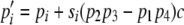for i = 1, … , 4 in which s₁ = s₄ = 1 and s₂ = s₃ = –1 (cf. Ewens 2004). When a large reproduction event occurs, a single randomly chosen haplotype represents a fraction ω of the common gamete pool and the other haplotypes compose the remaining 1 – ω fraction of gametes. In this case, the formula for above holds, but with p_i and p_j≠i replaced by 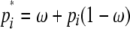and 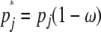for j ≠ i. Note that simultaneous multiple mergers (Schweinsberg 2000; Möhle and Sagitov 2001) are not possible in this simplified model of recombination.

Prediction of linkage disequilibrium:

The quantity r² given in Equation 1 is a ratio of two nonindependent random variables and has an unknown distribution, but Song and Song (2007) do make an advance in its numerical evaluation.

A first approximation to is the ratio of expectations 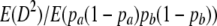(Ohta and Kimura 1971). We write . Considering the gene genealogy of a sample of size two of two loci, McVean (2002) showed that the ratio of expectations ϒ can be written in terms of covariances in pairwise coalescence times t₁ and t₂ at each of two loci,

(4)

in which 𝒮₀, 𝒮 ₁, and 𝒮₂ denote the three possible configurations in a sample of size two shown in Figure 2. In the case of small samples, Equation 4 can be corrected for the possibility that the same gamete is sampled more than once (Hudson 1985; McVean 2002). In deriving Equation 4, McVean (2002) assumed that the per-site mutation rate is very small.

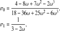
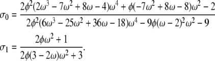
The covariance terms in Equation 4 have been derived under the standard coalescent (Griffiths 1981, 1991) (see also Pluzhnikov and Donnelly 1996; Durrett 2002). Let ρ denote the scaled recombination rate. Under standard Wright–Fisher sampling, in which time is measured in units of 2N generations, ρ = 2Nc. Then the corresponding correlations given each sample configuration (𝒮₀, 𝒮₁, or 𝒮₂; see Figure 2) are given by Equation A1 in the appendix (by replacing η with ρ/4). Hence,

(5)

(McVean 2002), which agrees with the results obtained by Ohta and Kimura (1971) and Weir and Hill (1986) by other methods. Simulations show that Equation 5 provides a good approximation to the average value of r² calculated from a sample when the frequency of the minor allele is not too small (Hudson 1985; McVean 2002).

Deriving the covariance terms under a modified population model:

The correlations in Equation A1 were obtained on the basis of the standard coalescent (Kingman 1982a,b; Hudson 1983; Tajima 1983), in which only binary mergers are allowed; hence the only parameter is the scaled recombination rate ρ (Griffiths 1981, 1991). The corresponding correlation terms derived under our modified Wright–Fisher population model are shown in the appendix. In this case, and in what follows, we define the scaled recombination parameter to be η = cN^β. We assume that η and φ are finite; i.e., and are both finite (recall that the probability of modified Wright–Fisher sampling is ɛ = φ/N^α). Note that the usual scaling of the recombination rate is obtained by taking β = 1. Defining the recombination parameter η in this way allows us to investigate effects of order of magnitude differences in timescales of recombination and coalescence. The parameter controlling the timescale of coalescence is α. When α ≥ 1 coalescence occurs on a timescale proportional to N generations. However, if 0 < α < 1, the timescale of coalescence is N^α generations (Table 1). To obtain a continuous-time limit we rescale time using the coalescent timescale. Thus the rate of coalescence shown in Table 1 is always finite. On the coalescent timescale the rate of recombination is cN^α = ηN^α–β (we can think of this as our model's analog of the usual parameter ρ). Since η is finite, if α > β, i.e., when recombination is an order of magnitude more frequent than coalescence. If α < β then 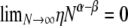, and coalescence events are an order of magnitude more frequent than recombination events. Coalescence and recombination occur on the same timescale only when α = β.

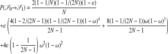
To explain the derivations, recall that ϒ can be expressed in terms of covariances (see Equation 4) and since Cov(X, Y) = E(XY) – E(X)E(Y) for any two random variables X and Y, we first obtain the expected values of the products of the pairwise coalescence times t₁ and t₂ at the two loci. That is, the main work involves obtaining E(t₁t₂ | S_i) for i = 0, 1, 2 (see Figure 2). Let s_ij denote the transition probability over a single generation between states in the ancestral process for two biallelic loci with recombination between them, under a standard population model (e.g., the Wright–Fisher model). Denote by m_ij the transition probability per generation under a modified sampling scheme. Then under a modified population model the transition probability p_ij over one generation from state i to state j is

(6)

The gene genealogical process we are describing is that for a sample of size two of two loci, or a total of four genetic types. The transition probabilities take the general form of Equation 6 in which s_ij and m_ij are given in the appendix, and the seven possible states are given in Figure 2.

By considering the corresponding Markov jump chain, we can follow Durrett (2002) to obtain E(t₁t₂ | 𝒮_i) in which t₁ and t₂ denote the time until coalescence of the two genetic types at loci 1 and 2, respectively. Conditioning on the first change in the genealogical history of the sample we obtain the set of recursions given in Equation 7,

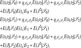(7)

in which 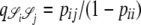, , , and . Since J denotes the time until the process moves out of a particular state, 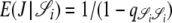and 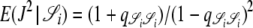. The quantity t_c is the time until two lines coalesce (ignoring recombination), for which E(t_c) = 1/G_2,2, and G_n,x given in Equation 2 is the probability that x lines of n coalesce in one generation. Note that Equation 4 can also be written as

(8)

Let E(t₁t₂ | 𝒮_i) denote the solution of Equation 7 for i = 0, 1, 2. The continuous-time limit prediction of linkage disequilibrium is then given by

(9)

The limit in Equation 9 will depend on the different values of α and β, the parameters controlling the timescale of coalescence and recombination, respectively. The different continuous-time limit predictions of linkage disequilibrium obtained from Equation 9 are given in Table 2, and the correlations are given in the appendix.

TABLE 2.

The continuous-time limit predictions of linkage disequilibrium ϒ under a modified Wright–Fisher population model

Timescale
Coalescence		Recombination	Limit process
α > 1		β > 1
		β = 1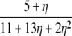
		β < 1	0
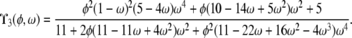
α = 1		β > 1	ϒ3(φ, ω)
		β = 1	ϒ2(η, φ, ω)
		β < 1	0
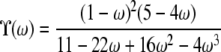
α < 1		β > 1	ϒ(ω)
		β = 1	ϒ(ω)
	0 < α < β < 1		ϒ(ω)
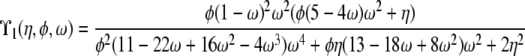
	0 < α = β < 1		ϒ1(η, φ, ω)
	0 < β < α < 1		0

The different formulas are the limit (9) obtained given different values of α and β. See text for explanation of symbols. Note that .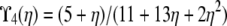

RESULTS

Correlations in coalescence times are strongly affected by demography, in this case extreme differences in reproductive success among individuals in a population. The correlations obtained under different assumptions about the two parameters, α and β, that control the timescales of recombination and random drift are shown in the appendix. When found to be functions of ω (the fraction of the population replaced by offspring of a single individual) and φ (recall that the probability of modified Wright–Fisher sampling is given by ɛ = φ/N^α), the correlations ascend to 1 as ω and φ increase.

Different predictions of LD:

Eleven different predictions (Equation 9) of linkage disequilibrium are identified (Table 2), depending on α and β (recombination is scaled as η = cN^β). These results are summarized in Figure 3 on the parameter space spanned by α and β. The timescale in a standard Wright–Fisher diploid population is 2N generations. Thus when α > 1 ω-coalescence events are an order of magnitude less frequent than binary mergers, and the ancestral process is Kingman's coalescent. The coalescent timescale when 0 < α < 1 is in units of N^α generations, and the ancestral process is dominated by ω-coalescence events allowing for multiple mergers. Kingman's coalescent and ω-coalescence events occur on the same timescale (proportional to N generations) when α = 1. Recombination occurs on a faster timescale (by an order of magnitude) than any type of coalescent event on the region of the (α, β) parameter space represented by zero (β < 1 except 0 < α < β < 1) in Figure 3. Thus this region is labeled as “frequent recombination” in Figure 3. The remaining part of the (α, β) parameter space is labeled as “infrequent recombination” to remind us of the longer timescale (for this part of the parameter space) on which recombination occurs relative to the corresponding coalescent timescale.

Figure 3.—

Predictions of linkage disequilibrium from Table 2 on the (α, β) parameter space. The circled numbers refer to ϒ_j (j = 1, … , 4) as shown in Table 2. For explanation of symbols see text.

Just three possible limiting behaviors—0, , and ϒ(ω)—occupy nearly all of the (α, β) parameter space (Figure 3). Linkage equilibrium (r² = 0) is predicted when 0 < β < α < 1 or when 0 < β < 1 and α ≥ 1—this is the region of the (α, β) parameter space occupied by 0 in Figure 3. In these cases, the rate of recombination is an order of magnitude higher than any type of coalescence event () and hence we do not expect to see any disequilibrium. In contrast, high linkage disequilibrium is predicted when both α and β > 1, which is the region occupied by in Figure 3. Here the timescale of coalescence is proportional to N generations, the ancestral process is Kingman's coalescent, and recombination occurs on a timescale that is an order of magnitude longer than the coalescent timescale; i.e., . Note that is the value obtained from Equation 7 when ρ = 0. Finally, when 0 < α < β and α < 1, the prediction of linkage disequilibrium is a function of ω (the fraction of the population replaced by offspring of a single individual)—the region occupied by ϒ(ω) (Table 2) in Figure 3. The ancestral process occurs on a timescale of N^α generations and is characterized by ω-coalescence events allowing for multiple mergers. Since β > α it follows that recombination occurs on a timescale that is longer (by an order of magnitude) than the coalescent timescale ().

When α and β are equal and ≤1, recombination and coalescence occur on the same timescale of N^α ≤ N generations, and more complicated behaviors are observed. The prediction of LD is then a function of all three parameters η, φ, and ω, and two different limit processes, ϒ₁(η, φ, ω) and ϒ₂(η, φ, ω) (Table 2), arise. The limit process ϒ₁(η, φ, ω) is obtained when 0 < α = β < 1, represented by the thick diagonal line labeled in Figure 3, and the limit process ϒ₂(η, φ, ω) represented by in Figure 3 results when α = β = 1.

When α = 1, the ancestral process is a mixture of the standard coalescent and a multiple-mergers coalescent process, since both occur on a timescale proportional to N generations. Taking α = 1 and restricting recombination to a longer timescale (β > 1) results in the limit process ϒ₃(φ, ω) (Table 2), which occupies the part of the (α, β) parameter space represented by the thick vertical line labeled in Figure 3. When α > 1 the standard coalescent process results, the timescale is proportional to N generations, and the population follows the usual Wright–Fisher reproduction framework. Scaling recombination in the usual way by taking β = 1 under the usual Wright–Fisher reproduction (α > 1) results in the standard prediction ϒ₄(η) (Table 2) of LD represented by the thick horizontal line labeled in Figure 3.

Nonmonotonic behavior of E(r²):

Interestingly, while linkage disequilibrium decreases monotonically as recombination increases, the predictions ϒ₁ and ϒ₂ are nonmonotonic functions of φ and ω. Figure 4a shows ϒ₁(η, φ, ω) as a function of φ (1 ≤ φ ≤ 10) and ω (0 < ω < 1) when η = 1, and Figure 4b shows ϒ₂(η, φ, ω) under the same conditions for η, φ, and ω as in Figure 4a. A comparison of the two graphs in Figure 4 shows that ϒ₁(η, φ, ω) and ϒ₂(η, φ, ω) behave very similarly as functions of φ and ω. The nonmonotonic trends emerging from Figure 4 are twofold. First, for any value of φ, ϒ₁(η, φ, ω) and ϒ₂(η, φ, ω) ascend as ω goes from 0 to ∼0.4 and then descend as ω goes from ∼0.4 to 1. The other nonmonotonic trend is that, depending on ω, ϒ₁(η, φ, ω) and ϒ₂(η, φ, ω) are either increasing or decreasing functions of φ. Thus, when multiple mergers and recombination occur on the same timescale of ≤2N generations, the prediction of linkage disequilibrium is nonmonotonic in the parameters that control the rate (φ) and size (ω) of multiple mergers.

Figure 4.—

Predicted levels of linkage disequilibrium (a) ϒ₁(η, φ, ω) and (b) ϒ₂(η, φ, ω), from Table 2 as a function of φ and ω when η = 1. For explanation of symbols see text.

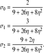
The nonmonotonic behavior of ϒ₁ and ϒ₂ is interesting because the correlation in coalescence times increases monotonically with φ and ω. Let σ_i = corr(t₁, t₂ | 𝒮_i), i = 0, 1, 2. Writing ϒ = σ₀/(1 + σ₀) + σ₂/(1 + σ₀) – 2σ₁/(1 + σ₀) and looking at each term separately one can see that, relative to 1 + σ₀, σ₂ rises most steeply over the same interval of ω for which ϒ is increasing (Figure 5).

Figure 5.—

Correlations in coalescence times σ_i, relative to 1 + σ₀, as functions of ω when η = 1, φ = 100, and β = α = 1 (see appendix). Line c₁, σ₀/(1 + σ₀); line c₂, σ₂/(1 + σ₀); line c₃, 2σ₁/(1 + σ₀); line c₄, (σ₂ + σ₀)/(1 + σ₀). For explanation of symbols see text.

The ancestral process occurs on a timescale of N^α generations when 0 < α < 1 and is characterized by ω-coalescence events allowing for multiple mergers. Thus when recombination occurs on a longer timescale (even if 0 < β < 1, cf. Figure 3) the prediction of linkage disequilibrium depends only on ω [for this range of the (α, β)-parameter space]. Figure 6a shows ϒ(ω) is a decreasing function of ω. When ω is very small, high LD is predicted since the gene genealogy resembles the one obtained under standard Wright–Fisher reproduction (see Figure 1b). As ω increases, the gene genealogy starts to resemble more the one shown in Figure 1a, i.e., consisting mostly of external branches because of multiple mergers, leaving little opportunity for LD to establish.

Figure 6.—

Predicted levels of linkage disequilibrium (a) ϒ(ω), (b) ϒ₂(η, φ, ω), and (c) ϒ₃(φ, ω) from Table 2 as a function of ω. In b η = 10 and φ = 1000. The horizontal dashed line in b represents the predicted level of linkage disequilibrium under the standard Wright–Fisher model (ϒ₄(η)) when η = 10. For explanation of symbols see text.

In Figure 4, η = 1, which gives ϒ₄(1) ≈ 0.231. Thus, for the range of φ chosen, predicted levels of linkage disequilibrium under modified Wright–Fisher sampling are generally less than those predicted under standard Wright–Fisher reproduction, given that recombination occurs on the same timescale as coalescence (0 < α = β ≤ 1). When recombination occurs on a shorter timescale than coalescence, ϒ is zero. By taking α = β when β ≤ 1 the effects of recombination are countered by setting the timescale of modified sampling equal to that of recombination.

Higher than expected LD:

For a certain range of the parameter space, higher predicted levels of linkage disequilibrium can also be obtained under modified sampling compared to the standard model. Figure 6b shows ϒ₂(η, φ, ω) as a function of ω with φ = 1000 and η = 10. The linkage disequilibrium predicted under the standard Wright–Fisher model (ϒ₄(η)) when η = 10 is shown for reference (Figure 6b, dashed line). For low and high values of ω the level of LD predicted under modified sampling is similar to or less than that predicted under the standard model. For intermediate values of ω, much higher levels of LD are predicted under modified sampling. The interpretation of Figure 6b is that high linkage disequilibrium can result from random sampling in a population with high variance in offspring number. Contrast this with Figure 6c, which shows a graph of ϒ₃(φ, ω) (Table 2) as a function of ω for three different values of φ. In this case of low recombination (β > 1), ϒ₃ is a decreasing function of ω and φ. For high values of ω and/or φ, the model predicts low linkage disequilibrium even under low recombination. Taken together, a population with highly skewed offspring distribution can have high LD in regions with high recombination and low LD in regions with low recombination.

Another interesting, and cautionary, aspect of our results is that the same prediction of linkage disequilibrium can be obtained with different combinations of parameters. For example, given a standard population model, ϒ₄(η) = if 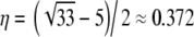. However, for any β > α, as long as α < 1, ϒ(ω) = when ω ≈ 0.2831 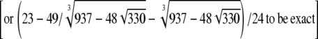This implies that it may be difficult to distinguish between η, φ, and ω using sequence data.

The distribution of r² in simulations:

The expected value of r² was the focus of the analytical work above. However, Hudson's (1985) analysis of the distribution of r² by simulation reveals a high variance of this measure of LD. To obtain quantitative estimates of the variance of r² we performed Monte Carlo simulations under a symmetric two-allele mutation model as described by Hudson (1983) with the modification of allowing more than two lines to coalesce at the same time. The program we wrote to perform the simulations correctly predicts the correlations listed in the appendix. A version in C is available upon request.

Table 3 shows results from simulations obtained under two different ancestral processes: one in which the rate of coalescence (x-merger) is given by 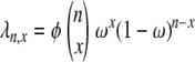for 2 ≤ x ≤ n and is labeled as “multiple mergers” in Table 3 and the other in which the rate of coalescence is given by Equation 10 and obtained when large reproduction events occur on a timescale of 2N generations. The entries in Table 3 are the mean of r² and the corresponding standard deviation in parentheses. In nearly all cases the standard deviation is larger than the mean, indicating a high variance in the empirical distribution of r². Figure 7 shows the sampling distribution of r² under the same two coalescent processes as in Table 3. The distributions are similar to those obtained by Hudson (1985) and reflect the high sampling variance of r². Following McVean (2002), our analytical results assume that the population mutation rate θ is small. The analytical predictions for we have derived are in good agreement with simulations for biologically reasonable values of ω (Table 3) as long as θ is small: not >10⁻² in the case of the mixture-distribution coalescent process or 10⁻³–10⁻⁴ if the ancestral process is the multiple-mergers process. For comparison, a value of ω of ∼8% was estimated for Pacific oysters (C. gigas; Eldon and Wakeley 2006).

TABLE 3.

Mean and standard deviation (in parentheses) of r² for a sample of size 25 (10⁴ iterations) under the “multiple-mergers” process (η = 0) and the mixture-distribution process (η = 1)

		Ancestral process
ω	θ	Multiple mergers	Mixture distribution
0.1	1	0.055 (0.073)	0.106 (0.143)
	0.1	0.073 (0.095)	0.107 (0.180)
	0.01	0.149 (0.195)	0.159 (0.238)
			0.230a (0.299)
	0.001	0.251 (0.352)
		0.409a (0.373)
	Predicted	0.416	0.232
0.5	1	0.073 (0.104)	0.162 (0.232)
	0.1	0.119 (0.196)	0.164 (0.269)
	0.01	0.125 (0.275)	0.183 (0.354)
			0.205a (0.279)
	0.001	0.176 (0.370)
		0.212a (0.341)
	Predicted	0.214	0.232

In each case φ = 1. The predicted values are ϒ(ω) for the multiple-mergers process and ϒ₂(1, 1, ω) for the mixture-distribution process (see Table 2).

^aLow-frequency (<10%) variants excluded.

Figure 7.—

The sampling distribution of r² for sample size 25 after 5 × 10⁴ runs under (a) a “multiple-merger” coalescent process (0 < α < 1) and no recombination (η = 0) and (b) a mixture-distribution coalescent process (α = 1) with η = 1. In a, θ = 0.001 and low-frequency variants (<10%) are excluded, while in b θ = 0.01 and all variants are included. In both cases ω = 0.1 and φ = 1. The vertical dashed lines represent the mean of each sampling distribution: (a) with standard deviation 0.377; (b) with standard deviation 0.132.

DISCUSSION

Limit predictions (as ) about linkage disequilibrium were obtained under a skewed offspring distribution among individuals in a population, in which the offspring of a single (randomly chosen) individual can number on the order of the population size. It is shown that the reproduction parameters ω and φ, which control the size and frequency of the large reproduction events, are as important as the recombination rate in predicting levels of LD in a population with highly fecund individuals. Primarily, low LD is predicted due to the star-like shape of the gene genealogy. This can occur, in some cases, despite a low recombination rate and can thus give false evidence for the presence of a recombination hotspot. High LD can also be predicted despite a high recombination rate (see discussion below), i.e., even in the presence of a recombination hotspot. The present results are qualitatively similar to the effects of a recent strong selective sweep on the LD between two neutral loci linked to the selected locus (McVean 2007).

For example, in the model we have described the actual timescale of the ancestral process depends on the parameter α, which determines the frequency of highly fecund individuals (Table 1; the probability of modified Wright–Fisher sampling is ɛ = φ/N^α). We have studied the effects of a highly skewed offspring distribution on correlations in coalescence times between two loci. The findings show that predictions of linkage disequilibrium are strongly affected by the different timescales on which recombination and random drift operate, as well as the fraction ω of the population replaced by offspring of a single individual. Thus allowing recombination and reproduction to occur on separate, and sometimes very different, timescales uncovers a fundamental way in which LD may be shaped by high variance in offspring number.

For a given α, correlations in coalescence times were shown to be increasing functions of φ (recall that the probability of modified Wright–Fisher sampling is ɛ = φ/N^α) and ω (the fraction of the population replaced by offspring of a single individual). The dependence of the correlations on φ and ω can be explained through the effects φ and ω have on the shape of the gene genealogy of a sample of two loci on two chromosomes. If the ancestral gametic type (state 𝒞₄ in Figure 2) is reached from any of the 𝒮_i sample configurations in Figure 2, with high probability in a large population, the coalescence times would be highly correlated. Reaching the common-ancestral chromosome (𝒞₄) from any of the 𝒮_i states requires only a single multiple merger and is possible in a large population given the population models considered in this report. As ω increases (i.e., tends to 1), the fraction of the population replaced by offspring of a single individual tends to 1. Hence, the gene genealogy assumes a star-like shape composed almost entirely of external branches (similar to the gene genealogy on the right in Figure 1), if ω-coalescence events are frequent enough. The rate of ω-events is determined by φ. It follows that as φ and ω increase, the more star-like the gene genealogy becomes, and the common-ancestral type 𝒞₄ is often reached via a single coalescence event from any given configuration 𝒮_i, resulting in high correlation in coalescence times.

Given a highly skewed offspring distribution, predicted levels of LD can range from high to low irrespective of recombination. Consider the case when ω-coalescence events occur on a shorter timescale than the standard coalescent; i.e., α < 1. In this case the rate φ of ω-coalescence events is much greater than the rate N^α–1 of the standard coalescent. In a standard Wright–Fisher population predictions of linkage disequilibrium depend only on the recombination rate (η). Common intuition says that when there will not be much LD. However, if 0 < α < β < 1, nonzero linkage disequilibrium can occur when if the timescale of coalescence is also short due to multiple mergers (Table 2). Given the modified model of reproduction considered in this study, predicted levels of LD depend on ω only when 0 < α < β < 1. For low values of ω the model predicts high LD (i.e., close to ), and as ω tends to 1 predicted levels of LD descend toward zero. Second, when (i.e., β > 1), predicted levels of LD also only depend on ω in the same way as when 0 < α < β < 1. Thus the model can predict low levels of LD (if ω ≈ 1) even when and common intuition says that LD should be high. The relation between recombination and linkage disequilibrium may not be as straightforward in organisms with highly fecund individuals as standard theory predicts.

Linkage disequilibrium as predicted by ϒ does not change monotonically with ω when recombination and multiple mergers occur on the same timescale of N^α ≤ N generations (0 < α = β ≤ 1; see Figure 4). When values of ω are not too close to 1, high LD can result as Figure 6b shows. Again following Slatkin (1994) a consideration of the gene genealogy of a sample of two completely linked loci can explain the high predicted LD when 0 < α = β ≤ 1. The modified Wright–Fisher model considered in the present study allows many lines to reach a common ancestor (coalesce) in the same instance. Thus given n ancestral lines, any number of lines from 2 to n can reach a common ancestor each time a coalescence event occurs. To explain the high predicted LD when 0 < α = β ≤ 1 we consider the probability (Figure 8) of each type of coalescence event (x-merger) for 2 ≤ x ≤ n given 10 ancestral lines (n = 10). On a timescale of 2N generations the rate λ_n,x of coalescence of x lines of n (2 ≤ x ≤ n) is given by

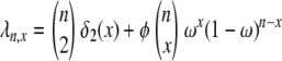(10)

[in which δ₂(x) = 1 if x = 2 and zero otherwise] obtained from Equation 2. Under the standard coalescent only two lines can reach a common ancestor (2-merger) each time a coalescence event occurs. Figure 8 (a, solid bars) shows, however, that when φ = 1000 (in accordance with Figure 6b) and ω = 0.5 the most likely coalescence event is that half the lines reach a common ancestor and that a 2-merger is among the least likely events. Similar patterns are obtained for lower values of φ and ω. The high probability of multiple mergers directly affects our prediction of the shape of the gene genealogy of a sample. Figure 8b shows the gene genealogy of a sample of two completely linked loci when ω = 0.5 and most multiple mergers are more likely than 2-mergers (or n-mergers). The gene genealogy consists of short external branches and a long internal branch at each locus. Assuming a single mutation at each locus, both mutations most likely occur in the internal branch, leading to high LD. The probability distribution of multiple mergers for φ = 1000 and ω = 0.99 is shown for reference (Figure 8, shaded bars). When the offspring of a single individual frequently replace almost all the population, the most likely coalescence event is an n-merger, i.e., all ancestral lines reaching a common ancestor. The gene genealogy of a sample then becomes star shaped, similar to the gene genealogy in Figure 1a. Mutations are then most likely to occur in an external branch, resulting in low linkage disequilibrium.

Figure 8.—

Rates of coalescence and gene genealogy under a multiple-mergers coalescent. (a) The probability distribution of the different types of coalescence events, given by 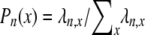(2 ≤ x ≤ n) in which [δ₂(x) = 1 if x = 2 and zero otherwise] in units of 2N generations (i.e., α = β = 1) when the number of ancestral lines n = 10 and φ = 1000. Solid bars, ω = 0.5; shaded bars, ω = 0.99. (b) A gene genealogy of a sample of two completely linked loci given a multiple-mergers ancestral process similar to the one described by solid bars in a. One mutation event is assumed at each locus, and the ancestral gametic type is AB.

Analytical results presented here rely on the approximations of Ohta and Kimura (1971), who suggested using a ratio of expectations as a predictor for r², and McVean (2002), who assumed a small mutation rate. In addition, the analytical predictions are only for the average value of r². These issues were addressed using simulations. The results show that the expected value of r² is in agreement with the analytical results when θ is small and the offspring of a single individual replace a modest fraction (ω) of the population (0 < ω ≤ 0.5; Table 3). However, the sampling variance of r² is quite high (Table 3 and Figure 7), similar to that found for the standard coalescent (Hudson 1985). In the analysis of data, the variance of r² can be reduced by averaging values over very many pairs of loci.

APPENDIX

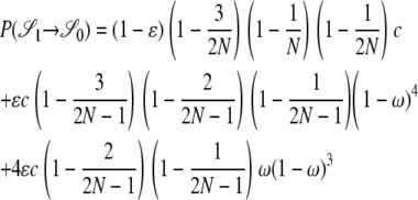
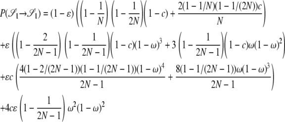
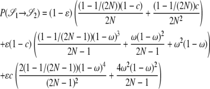
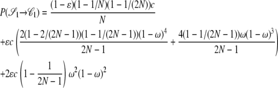
Transition probabilities:

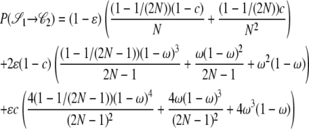
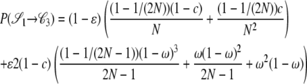
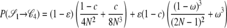
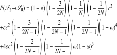
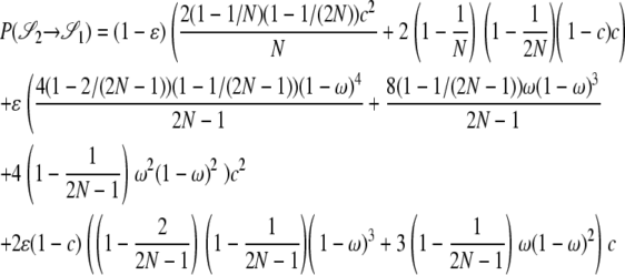
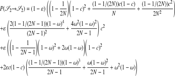
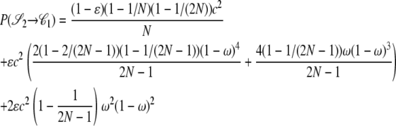
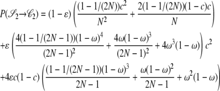
Here the transition probabilities from the noncoalescent states , , and (Figure 3) in the ancestral process are stated. These are in discrete time. The states are based on two biallelic loci in a sample of size two from diploid individuals. Only one crossover is allowed between the loci when a recombination event occurs. A transition probability from state i to state j is denoted . And of course . 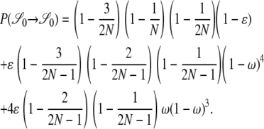As an example, consider or the probability that all four alleles stay on separate chromosomes over one generation. Standard Wright–Fisher sampling occurs with probability 1 – ɛ and modified sampling with probability ɛ. The two separate probabilities can be obtained by adopting a balls-in-boxes approach. Going one generation back in time, the four balls (alleles) occupy 2N boxes (chromosomes) at random. To stay in state , no recombination is involved, and all the balls must occupy different boxes. Under standard sampling, this happens with probability . Under modified sampling, a single randomly chosen box is occupied by a ball with probability ω (the ω-box), while the other 2N – 1 boxes are each occupied by a ball with probability 1/(2N – 1). Under modified sampling, the four balls stay in separate boxes in two ways. First, they can all ignore the ω-box with probability (1 – ω)⁴ and then must all occupy different boxes with probability . Second, a single randomly chosen ball occupies the ω-box with the binomial probability 4ω(1 – ω)³, while, of the remaining three balls, each occupies a single box with probability

The other transition probabilities are obtained similarly:

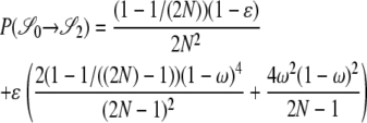
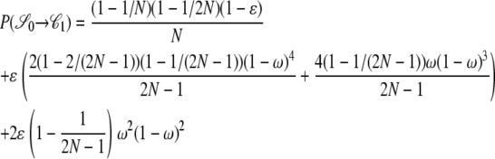
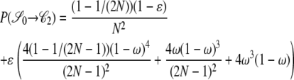
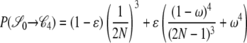
Correlations in coalescent times:

Here the correlations in coalescent times between the two loci are specified for the modified Wright–Fisher population model. These are the correlations given that the ancestral process starts from one of the three noncoalescent states ,or (Figure 3) and are obtained as a limit process in a large population (i.e., as ). In what follows, let σ₀ = corr(t₁, t₂ | ), σ₁ = corr(t₁, t₂ | ), and σ₂ = corr(t₁, t₂ | ). The different cases depend on the values of the recombination-timescale parameter β (recombination is scaled as η = cN^β), and the reproduction-timescale parameter α (the probability of modified Wright–Fisher sampling is ɛ = φ/N^α), and are of course the same as those given for ϒ. Note that the correlation terms can be used to obtain ϒ using Equation 11 in McVean (2002). Replacing η with η/2 and φ with φ/2 gives the formulas for ϒ in Table 2. The factor of 2 comes from the timescale of 2N (in the case α ≥ 1) used in obtaining the correlation terms. Predictions of the models concerning levels of linkage disequilibrium are independent of the different scaling of the parameters.

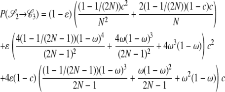
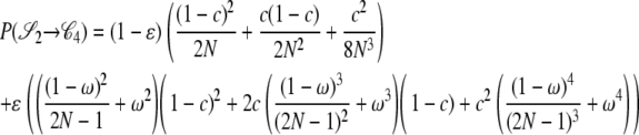
Only if 0 < α = β ≤ 1 the correlation terms are functions of all three parameters η, φ, and ω. If 0 < α = β < 1 the correlation terms are

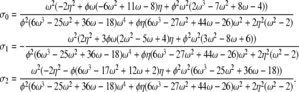If α = β = 1 the correlation terms are σ₀ = a₀/d – 1, σ₁ = a₁/d – 1, and σ₂ = a₂/d – 1 in which

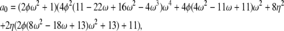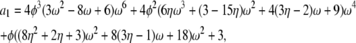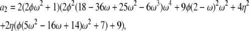If 0 < α, β < 1, and β < α, the three correlation terms are all equal to ω²/(2 – ω²). If 0 < α, β < 1, and α < β, the correlation terms are

and σ₂ = 1. This is always the case when α < β or when both parameters are >1. In the case α = 1 and β > 1,

If α > 1 and 0 < β < 1, all three correlation terms = 0.

If α > 1 and β = 1, the results correspond to those obtained under standard Wright–Fisher sampling:

(A1)

If α > 1 and β > 1, σ₀ = , σ₁ = , and σ₂ = 1.

References

- Árnason, E., 2004. Mitochondrial cytochrome b variation in the high-fecundity Atlantic cod: trans-Atlantic clines and shallow gene genealogy. Genetics 166 1871–1885. [DOI] [PMC free article] [PubMed] [Google Scholar]
- Bataillon, T., T. Mailund, S. Thorlacius, E. Steingrimsson, T. Rafnar et al., 2006. The effective size of the Icelandic population and the prospects for LD mapping: inference from unphased microsatellite markers. Eur. J. Hum. Genet. 14 1044–1053. [DOI] [PubMed] [Google Scholar]
- Crow, J. F., and M. Kimura, 1970. Introduction to Population Genetics Theory. Harper & Row, New York.
- Durrett, R., 2002. Probability Models for DNA Sequence Evolution. Springer, New York.
- Eldon, B., and J. Wakeley, 2006. Coalescent processes when the distribution of offspring number among individuals is highly skewed. Genetics 172 2621–2633. [DOI] [PMC free article] [PubMed] [Google Scholar]
- Ewens, W. J., 2004. Theoretical introduction in Mathematical Population Genetics, Vol. I, edited by S. S. Antman, J. E. Marsden, L. Sirovich and S. Wiggins. Springer, New York.
- Fisher, R. A., 1930. The Genetical Theory of Natural Selection. Clarendon Press, Oxford.
- Garđarsdóttir, O., and B. Sigurjónsson (Editors), 2006. Population (Statistical Series, Vol. 91). Statistics Iceland, Reykjavík, Iceland (in Icelandic).
- Griffiths, R. C., 1981. Neutral two-locus multiple allele models with recombination. Theor. Popul. Biol. 19 169–186. [Google Scholar]
- Griffiths, R. C., 1991. The two-locus ancestral graph, pp. 100–117 in Selected Proceedings on the Symposium on Applied Probability (Monograph Series, Vol. 18), edited by I. V. Basawa and R. L. Taylor. IMS Lecture Notes, Institute of Mathematical Statistics, Hayward, CA.
- Hedgecock, D., 1994. Does variance in reproductive success limit effective population sizes of marine organisms?, pp. 1222–1344 in Genetics and Evolution of Aquatic Organisms, edited by A. Beaumont. Chapman & Hall, London.
- Hedrick, P. W., 2000. Genetics of Populations, Ed. 2. Jones & Bartlett, Sudbury, MA.
- Hedrick, P. W., 2005. Large variance in reproductive success and the Ne/N ratio. Evolution 59 1596–1599. [PubMed] [Google Scholar]
- Hill, W. G., and A. R. Robertson, 1968. Linkage disequilibrium in finite populations. Theor. Appl. Genet. 38 226–231. [DOI] [PubMed] [Google Scholar]
- Hudson, R. R., 1983. Properties of the neutral allele model with intergenic recombination. Theor. Popul. Biol. 23 183–201. [DOI] [PubMed] [Google Scholar]
- Hudson, R. R., 1985. The sampling distribution of linkage disequilibrium under an infinite allele model without selection. Genetics 109 611–631. [DOI] [PMC free article] [PubMed] [Google Scholar]
- Jónsson, G., and M. S. Magnússon (Editors), 1997. Hagskinna: Icelandic Historical Statistics. Statistics Iceland, Reykjavík, Iceland (in Icelandic).
- Jorde, L. B., 1995. Linkage disequilibrium as a gene mapping tool. Am. J. Hum. Genet. 56 11–14. [PMC free article] [PubMed] [Google Scholar]
- Kingman, J. F. C., 1982. a The coalescent. Stoch. Proc. Appl. 13 235–248. [Google Scholar]
- Kingman, J. F. C., 1982. b On the genealogy of large populations. J. Appl. Probab. 19A 27–43. [Google Scholar]
- Lander, E. S., 1996. The new genomics: global views of biology. Science 274 536–539. [DOI] [PubMed] [Google Scholar]
- Lewontin, R. C., and K. Kojima, 1960. The evolutionary dynamics of complex polymorphisms. Evolution 14 450–472. [Google Scholar]
- McVean, G., 2007. The structure of linkage disequilibrium around a selective sweep. Genetics 175 1395–1406. [DOI] [PMC free article] [PubMed] [Google Scholar]
- McVean, G. A., 2002. A genealogical interpretation of linkage disequilibrium. Genetics 162 987–991. [DOI] [PMC free article] [PubMed] [Google Scholar]
- Möhle, M., 2006. On the number of segregating sites for populations with large family sizes. Adv. Appl. Probab. 38 750–767. [Google Scholar]
- Möhle, M., and S. Sagitov, 2001. A classification of coalescent processes for haploid exchangeable population models. Ann. Appl. Probab. 29 1547–1562. [Google Scholar]
- Moran, P. A. P., 1958. Random processes in genetics. Proc. Camb. Philos. Soc. 54 60–71. [Google Scholar]
- Moran, P. A. P., 1962. Statistical Processes of Evolutionary Theory. Clarendon Press, Oxford.
- Ohta, T., and M. Kimura, 1971. Linkage disequilibrium between two segregating nucleotide sites under the steady flux of mutations in a finite population. Genetics 68 571–580. [DOI] [PMC free article] [PubMed] [Google Scholar]
- Pitman, J., 1999. Coalescents with multiple collisions. Ann. Probab. 27 1870–1902. [Google Scholar]
- Pluzhnikov, A., and P. Donnelly, 1996. Optimal sequencing strategies for surveying molecular genetic diversity. Genetics 144 1247–1262. [DOI] [PMC free article] [PubMed] [Google Scholar]
- Risch, N., and K. Merikangas, 1996. The future of genetic studies of complex human diseases. Science 273 1516–1517. [DOI] [PubMed] [Google Scholar]
- Sagitov, S., 1999. The general coalescent with asynchronous mergers of ancestral lines. J. Appl. Probab. 36 1116–1125. [Google Scholar]
- Schweinsberg, J., 2000. Coalescents with simultaneous multiple collisions. Electron J. Probab. 5 1–50. [Google Scholar]
- Slatkin, M., 1994. Linkage disequilibrium in growing and stable populations. Genetics 137 331–336. [DOI] [PMC free article] [PubMed] [Google Scholar]
- Song, Y. S., and J. S. Song, 2007. Analytic computation of the expectation of the linkage disequilibrium coefficient r2. Theor. Popul. Biol. 71 49–60. [DOI] [PubMed] [Google Scholar]
- Strobeck, C., and K. Morgan, 1978. The effect of intragenic recombination on the number of alleles in a finite population. Genetics 88 829–844. [DOI] [PMC free article] [PubMed] [Google Scholar]
- Tajima, F., 1983. Evolutionary relationship of DNA sequences in finite populations. Genetics 105 437–460. [DOI] [PMC free article] [PubMed] [Google Scholar]
- Thorarinsson, S., 1961. Population changes in Iceland. Geogr. Rev. 51 519–533. [Google Scholar]
- Thorsteinsson, B., and B. Jónsson, 1991. Íslands Saga. Sögufélag, Reykjavík, Iceland (in Icelandic).
- Turner, T. F., J. P. Wares and J. R. Gold, 2002. Genetic effective size is three orders of magnitude smaller than adult census size in an abundant, estuarine-dependent marine fish (Sciaenops ocellatus). Genetics 162 1329–1339. [DOI] [PMC free article] [PubMed] [Google Scholar]
- Weir, B. S., and W. G. Hill, 1986. Nonuniform recombination within the human β-globin gene cluster. Am. J. Hum. Genet. 38 776–778. [PMC free article] [PubMed] [Google Scholar]
- Wright, S., 1931. Evolution in Mendelian populations. Genetics 16 97–159. [DOI] [PMC free article] [PubMed] [Google Scholar]