A New Bayesian Method to Identify the Environmental Factors That Influence Recent Migration

Abstract

We present a new multilocus genotype method that makes inferences about recent immigration rates and identifies the environmental factors that are more likely to explain observed gene flow patterns. It also estimates population-specific inbreeding coefficients, allele frequencies, and local population F_ST's and performs individual assignments. We generate synthetic data sets to determine the region of the parameter space where our method is and is not able to provide accurate estimates. Our simulation study indicates that reliable results can be obtained when the global level of genetic differentiation (F_ST) is >1%, the number of loci is only 10, and sample sizes are of the order of 50 individuals per population. We illustrate our method by applying it to Pakistani human data, considering altitude and geographic distance as explanatory factors. Our results suggest that altitude explains better the genetic data than geographic distance. Additionally, they show that southern low-altitude populations have higher migration rates than northern high-altitude ones.

THE study of dispersal processes is an essential problem in ecology, population genetics, conservation, and management of wildlife. For this reason, the estimation of migration rates has been one of the most investigated problems in population biology. Migration parameters can be directly estimated using ecological approaches such as mark-release-recapture methods but they are not applicable to the study of large or extended metapopulations. In these cases, population genetics approaches provide a better alternative because the information contained in DNA can provide gene flow parameter estimates for different and complementary timescales. Methods based on coalescent theory provide long-term migration rates because they use the genealogical information contained in a sample of genes (e.g., MIGRATE, Beerli and Felsenstein 2001). On the other hand, methods based on multilocus genotypes (e.g., BAYESASS, Wilson and Rannala 2003) provide estimates of recent immigration rates by extracting the gametic disequilibrium signal generated by immigrant individuals or their descendants.

Besides simply estimating migration rates, it is very important to identify the biotic and/or abiotic factors that influence them. This can be done by first obtaining gene flow estimates and then searching for correlations between them and various environmental variables (e.g., Giordano et al. 2007). Such an approach requires the use of summary statistics that do not take advantage of all the information contained in genetic data. An alternative approach is to implement the joint analysis of genetic and nongenetic data. Several current methods that combine both genetic and geographic data can be used to detect recent migrants (e.g., GENELAND, Guillot et al. 2005; TESS, François et al. 2006) but they do not take into account other environmental factors.

In previous studies we presented methods that use genetic and environmental data to study colonization processes (Gaggiotti et al. 2002, 2004) and population genetic structure (Foll and Gaggiotti 2006). These approaches based on hierarchical Bayesian methods (e.g., Gelman et al. 1995) estimate the probability that a given environmental factor influences the parameters of interest (e.g., composition of colonizing groups or local population F_ST's) because they explicitly model the relationship between them and the relevant ecological factors. In this article we present a new multilocus genotype method for inferring recent immigration rates and identifying the environmental factors that best explain observed gene flow patterns. We use a hierarchical Bayesian approach that introduces nongenetic data through the prior distribution of the migration rates. Following Wilson and Rannala's (2003) approach we implement the estimation of inbreeding coefficients to allow for departures from Hardy–Weinberg equilibrium within local populations. Finally, the method infers the population ancestry of individuals by assigning their alleles to populations from which they originated. We carry out a simulation study to identify the region of parameter space where the method is and is not able to provide accurate posterior estimates. We also illustrate our method with a real data example.

DATA AND MODEL PARAMETERS

Inferring migration rates from genetic data:

The method is based on a population genetics model that differs from that used by Wilson and Rannala (2003). More specifically, instead of assuming that sampling takes place right after migration, we consider that this is done after reproduction and before migration. Let us consider a metapopulation of a diploid species with nonoverlapping generations that is subdivided into I demes that can exchange migrants. Let be the observed multilocus genotypes of n individuals scored at L marker loci, where denotes the genotype of individual h at locus l. We assume that n_i individuals were sampled from population i and use the vector to identify the population S_h where the individual h was sampled from.

Population allele frequencies are given by a matrix composed of vectors that give the frequency of allele a at locus l for population i. Following Falush et al. (2003), we consider a model with correlated allele frequencies based on the approach introduced by Balding and Nichols (1995). Thus, we assume that before the last generation, the population was at migration–drift equilibrium so that allele frequencies in each population are determined by the global allele frequencies in the metapopulation as a whole, , and the degree of genetic differentiation between each local population and the overall metapopulation, , where θ_i = − 1. Finally, to allow departures from Hardy–Weinberg equilibrium, we introduce population-specific inbreeding coefficients , where F_i is the inbreeding coefficient for population i. Thus, we consider two levels of inbreeding, one at the population level corresponding to F_ST and another one at the individual level, corresponding to F_IS.

Instead of focusing directly on individual migration rates, we consider the probability that genes in a deme originated in another one over the last generation. Thus, migration is described by a matrix , where m_ij is the probability that alleles in population i came from population j during the previous generation. The ancestral state of the individuals is described by a matrix , where is a two-element vector identifying the source demes (i and j) for the two alleles of individual h. All possible ancestry states are considered: both alleles come from the deme where the individual was sampled, or both come from another deme, or they come from two different ones. Thus, migration rates for individuals are obtained as

(1)

where is the probability that individuals sampled from population i belong to the ancestry class (j, k). Note that our approach estimates migration rates only over the last generation. Moreover, as opposed to Wilson and Rannala (2003) migration rates vary freely in the interval (0, 1) and do not have to be small.

The model parameters described above () are estimated from the genetic data using a Bayesian approach and Markov chain Monte Carlo (MCMC) techniques.

Likelihood:

The likelihood is the probability of the observed genotypes given model parameters and is constructed by defining the probability of observing the genotype of individual h at locus l in terms of the ancestry classes. We note these genotypes , where X_hlc is the allele observed at locus l in chromosome c = 1, 2 of individual h. Thus, individual h genotype likelihood at locus l is given by

(2)

where

(3)

and

(4)

The first case considered in Equation 2 corresponds to the scenario where both alleles originated in the same source population, in which case we need to take into account possible deviations from Hardy–Weinberg equilibrium (see Equation 3). The second case considers that the individual is the descendant of parents that come from two different source populations, in which case we need to take into account that there are two different ways of assigning the alleles to the parents.

If we assume that individuals were sampled at random and loci are unlinked, then the likelihood of the whole sample is obtained by multiplying across all loci and individuals,

(5)

This likelihood can be used as the basis for inference using a Bayesian approach.

Combining genetic and environmental data:

One can expect that migration patterns are influenced by environmental factors such as population densities, distances between local populations, etc. To identify which environmental factors have influenced gene flow we use Gaggiotti et al.'s (2004) approach. Let us suppose that our knowledge of the species under study leads us to think that R environmental factors may influence the migration process. We can then introduce their effect through the prior distribution of gene migration rates. More specifically, we focus on the ancestry of immigrant alleles by conditioning on not being a resident allele

(6)

and assume that the vector follows a Dirichlet distribution; i.e., , where are shape parameters for the Dirichlet distribution. Furthermore, we assume that each shape parameter ψ_ij follows a lognormal distribution; i.e., for each pair of distinct populations i ≠ j

(7)

where the mean μ_ij is given by the generalized linear regression

(8)

where α_r denotes the effect of environmental factor r and α_rs denotes the effect of first-order interactions between factors r and s; these parameters are collected into a single vector . The sign and the magnitude of the α's tell us about the direction and the strength of the environmental factors. Finally, σ² is the amount of variation that remains unexplained by the regression and is the observed value for factor r, which is hypothesized to influence migration between populations i and j. To reduce posterior correlation and to simplify prior elicitation and posterior interpretation process, explanatory factors are normalized before analysis so that they have zero mean and variance one.

By excluding different regression terms we can define different alternative models. We note, however, that as opposed to previous applications of this approach (cf. Gaggiotti et al. 2004; Foll and Gaggiotti 2006), the intercept α₀ is included in all models because it takes into account the effect of factors that act at a geographic scale larger than that of the metapopulation under study (see discussion for more details).

Other priors:

We assume that there is no prior information on the shape of the other parameters and, therefore, adopt the vague priors that are given in the appendix. Note that in the particular case of the probability to observe nonmigrant genes (i.e., m_qq), we adopt a uniform prior between 0 and 1 because, although some environmental factors may influence whether or not an individual decides to emigrate, our method is aimed at estimating immigration rates and, therefore, cannot take into account this possibility.

Posterior distribution:

The model is now expressed in terms of parameters and the corresponding posterior distribution is given by Bayes' rule:

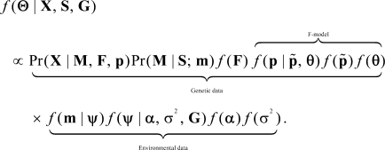(9)

The full model is represented by the directed acyclic graph (DAG) in Figure 1.

Figure 1.—

The DAG for the model given in Equation 9. Square nodes denote known quantities (i.e., data) and circles represent model parameters to be estimated. Arrows between nodes represent direct stochastic relationships within the model. The variables within each node correspond to model parameters discussed in the text.

The posterior distributions of parameters given in Equation 9 are estimated using MCMC methods that are described in the supplemental information.

Posterior model probabilities:

Besides estimating migration rates our method is aimed at identifying the environmental factors influencing gene flow. As we mentioned before, several alternative models can be obtained from the full regression (8) by canceling elements of the vector . Note that models that include first-order interactions between factors r and s are allowed only if both factors are included. Thus for model ℳ, the corresponding posterior distribution is given by

(10)

where is the parameter vector under model ℳ, is the corresponding regression vector, and denotes prior model probability. Posterior model probabilities are estimated using the reversible-jump (RJ)MCMC approach (Green 1995, detailed in supplemental information). Here we note only that one of the problems faced when estimating posterior model probabilities is that the prior for can have a large effect on the estimates. When very vague priors are used, more posterior weight is placed on the model with the fewest parameters. This is the well-known Jeffreys–Lindley paradox (Robert 1994). This problem was avoided by first running an MCMC of the full model with vague priors and then using the posterior estimates of the α's as informative priors for a new MCMC run.

SIMULATION STUDY

We evaluated the sensitivity of our method by generating synthetic data under a particular scenario in which gene flow is influenced by two factors. We considered various levels of genetic differentiation and migration rates. We are interested in the ability of our algorithm to find the correct scenario and to provide accurate posterior estimates for migration rates (with corresponding fairly narrow highest posterior density intervals, HPDI).

Generation of synthetic data:

We simulated data following the inference model presented in Figure 1. We initially considered a scenario with I = 4 populations, each with local population sizes of N_i = 5000 individuals. The sample size per population was n_i = 100 and we assumed that each sampled individual was scored for L = 10 polymorphic loci, each with K = 10 alleles.

Generating migration rates from environmental factors:

We consider two environmental factors that could be, for example, geographic distance (G₁) and population density (G₂). The pairwise geographic distances were generated using a standard normal distribution. The pairwise differences in population density were generated by first filling the top triangular matrix with values drawn from a standard normal and then filling the bottom triangular matrix with the opposite values. This procedure is equivalent to standardizing the observed pairwise differences in environmental factors before analysis.

To generate the migration matrix, we first chose the values for the diagonal elements (proportion of nonmigrant genes) and then we calculated the values for the nondiagonal elements (immigration rates) using the following procedure. We set α₁ = −0.9, α₂ = 1.1, and α₁₂ = 0 (i.e., no interaction effect) and calculated μ_ij's using Equation 8. Assuming no deviation from the linear regression (i.e., σ² = 0), we set . Finally we computed the means of the Dirichlet distribution used for the migration rates (Equation A2) and rescaled them so that they added up to 1 − m_ii.

Genetic data:

To generate multilocus genotypes with a given level of genetic differentiation, we need to generate parametric allele frequencies. This task was performed using Balding and Nichols' (1997) sampling formula for F_ST. According to this formula, genes are sampled one by one during an iterative process. The probability that the next gene sampled is a after having sampled n genes of which n_a correspond to allele a is given by

(11)

where p_a is the global frequency of allele a in the metapopulation.

To generate the parametric allele-frequency distribution of each locus in any given local population for a given F_ST value, we first sample an allele at random from the metapopulation allele-frequency distribution and then use Equation 11 to calculate the probability distribution for the type of the allele that will be sampled next. Using this distribution we obtain the next allele. This process is repeated iteratively until we obtain the 2N_i alleles present in local population i. We used uniform allele frequencies for the metapopulation.

Large departures from the target F_ST value were avoided by using the following iterative process. We generated the local population's allele-frequency distributions and calculated the global and pairwise F_ST's. If one or more of these values were not within 10% of the target value we discarded the allele frequencies and generated new ones. If the new allele frequencies satisfied the requirement, we generated the genotypes; otherwise we continued this iterative procedure until the constraint was satisfied. This procedure was used to control for the effect of genetic differentiation on the performance of the method.

Using the gene migration rates calculated above, we obtained the proportion of migrant individuals in each population using Equation 1. Multilocus genotypes for each local population were generated assuming Hardy–Weinberg equilibrium. Genotypes of nonmigrant individuals were obtained by drawing two alleles from the local population allele-frequency distribution. For the migrant individuals with both parents coming from the same local population, the genotype was obtained by drawing two alleles at random from the parents' source population. For migrant individuals with parents coming from different source populations, we sampled one allele from the source population of each parent. Finally, samples were generated by drawing n_i individuals from each local population, keeping track of the ancestry of both alleles for each sampled individual.

Implementation details:

Each MCMC was run for 1,030,000 iterations. The first 20,000 iterations consist of short pilot runs used to tune up the proposal distributions to obtain acceptance rates between 25 and 45%. The next 10,000 iterations were discarded as burn-in and the remaining observations were sampled every 100 iterations, giving a sample size of 10,000 for each analysis.

To take into account model uncertainty, parameters are estimated using Bayesian model-averaging methods. The only exception to this rule are the regression parameters, which are model specific and, therefore, were estimated using the subset of values corresponding to the model with the highest posterior probability. Finally, posterior model probabilities are obtained by observing the number of times the chain visits each alternative model.

Posterior estimates are based on the sample mean except for the deviation from the regression σ², which usually has a highly asymmetric posterior distribution. In this latter case we used the posterior mode, which was estimated using kernel density estimation.

We investigated the effect of varying three parameters: the level of genetic differentiation, F_ST = 〈0.01, 0.05, 0.10, 0.25〉; the proportion of nonmigrant alleles, m_ii = 〈0.7, 0.9〉; and the number of populations, I = 〈4, 6〉.

For each parameter set we generated 10 independent genetic data sets as described above. The results we present below are averages across these 10 replicates. As a measure of accuracy we also present the relative mean square errors (RMSE).

Results:

We investigated the performance of our method to provide reliable estimates under different scenarios of migration and genetic differentiation and number of populations studied. We consider first the effects on model determination, and then we address the influence on migration rate estimates and finally on individual assignments.

When the immigration rate is high (m_ii = 0.7; see Table 1), estimates of posterior model probabilities are strongly influenced by the degree of genetic differentiation (F_ST). When differentiation is low (F_ST = 0.01), the method fails to identify the model used to generate the synthetic data. However, the correct model is identified when F_ST > 0.01, and, moreover, its posterior model probability increases steadily with increasing genetic differentiation. The estimation of regression parameters is also influenced by the magnitude of F_ST but to a lesser degree. The RMSE decreases with increasing genetic differentiation but the bias is largely unaffected. Thus, it is the accuracy of the estimates (as illustrated by the HPDIs) that is influenced by F_ST. The proportion of the variance that remains unexplained by the model, σ², decreases as genetic differentiation increases.

TABLE 1.

Posterior estimates for various levels of genetic differentiation and high gene flow

		FST
Factors included		0.01	0.05	0.10	0.25
None		0.621	0.073	0.026	0.015
G1		0.142	0.061	0.028	0.016
G2		0.170	0.184	0.082	0.052
and		0.045	0.472	0.637	0.701
With interaction		0.022	0.210	0.227	0.216
		Estimate/RMSE/95% HPDI
Parameter	True value	0.01	0.05	0.10	0.25
α1	−0.900	a	−0.921	−0.974	−0.945
			0.057	0.027	0.003
			(−1.754; −0.097)	(−1.639; −0.324)	(−1.503; −0.370)
α2	1.100	a	1.137	1.178	1.149
			0.013	0.011	0.002
			(0.285; 2.068)	(0.504; 1.869)	(0.554; 1.745)
σ2	—	0.389	0.426	0.355	0.306
		—	—	—	—
		(0.120; 1.159)	(0.121; 2.858)	(0.106; 2.010)	(0.107; 1.578)
Assignments		0.01	0.05	0.10	0.25
Misassignments		0.754	0.280	0.110	0.002
Probabilitiesb		0.223	0.700	0.883	0.996

Posterior model probabilities, regression parameter mean estimates, and assignment accuracy for synthetic data generated with proportions of nonmigrant alleles set to m_ii = 0.70 are shown.

^aThe regression parameter is not included in the model with the highest posterior model probability.

^bMaximum posterior assignment probabilities averaged across all individuals.

Decreasing the immigration rate (m_ii = 0.90) has a detrimental effect on estimates (Table 2). Although the true model is correctly identified for F_ST > 0.01, its posterior probability is lower than that observed when m_ii = 0.70. Estimates of regression parameters are more biased and less accurate (wider HPDIs), leading to higher RMSEs. Also, the proportion of the variance that remains unexplained, σ², is larger. Note, however, that as was the case before, the quality of all estimates improves with increasing genetic differentiation.

TABLE 2.

Posterior estimates for various levels of genetic differentiation and low gene flow

		FST
Factors included		0.01	0.05	0.10	0.25
None		0.444	0.106	0.056	0.028
G1		0.122	0.072	0.055	0.030
G2		0.291	0.301	0.122	0.073
and		0.075	0.323	0.521	0.638
With interaction		0.068	0.197	0.246	0.231
		Estimate/RMSE/95% HPDI
Parameter	True value	0.01	0.05	0.10	0.25
α1	−0.900	a	−0.858	−1.122	−1.010
			0.123	0.101	0.015
			(−1.984; 0.263)	(−2.091; −0.191)	(−1.723; −0.321)
α2	1.100	a	1.403	1.314	1.173
			0.127	0.071	0.008
			(0.197; 2.687)	(0.387; 2.279)	(0.473; 1.886)
σ2	–	0.486	0.513	0.452	0.352
		—	—	—	—
		(0.131; 3.067)	(0.125; 4.117)	(0.120; 3.090)	(0.110; 1.956)
Assignments		0.01	0.05	0.10	0.25
Misassignments		0.808	0.134	0.046	0.002
Probabilitiesb		0.288	0.847	0.946	0.997

Posterior model probabilities, regression parameter mean estimates, and assignment accuracy for synthetic data generated with proportions of nonmigrant alleles set to m_ii = 0.90 are shown.

^aThe corresponding regression parameter is not included in the model with the highest posterior model probability.

^bMaximum posterior assignment probabilities averaged across all individuals.

Increasing the number of populations studied (I = 6) improves model determination (Table 3). More precisely, the posterior probability of the true model is strongly increased and the proportion of variance that remains unexplained decreases sharply (see Table 3 and last columns of Tables 1 and 2). However, the effect on the quality of the regression parameter estimates is somewhat decreased since the bias and the RMSE increase. Nevertheless, the width of the HPDIs decreases, indicating that the precision increases.

TABLE 3.

Posterior estimates for the scenario with six populations

		FST = 0.25
Factors included		mii = 0.70	mii = 0.90
None		0.000	0.000
G1		0.000	0.000
G2		0.000	0.001
G1 and G2		0.915	0.883
With interaction		0.085	0.116
		Estimate/RMSE/95%HPDI
Parameter	True value	mii = 0.70	mii = 0.90
α1	−0.900	−1.056	−1.022
		0.031	0.022
		(−1.416; −0.707)	(−1.521; −0.537)
α2	1.100	1.244	1.246
		0.018	0.018
		(0.960; 1.531)	(0.856; 1.659)
σ2	—	0.164	0.213
		—	—
		(0.080; 0.381)	(0.096; 0.566)
Assignments		mii = 0.70	mii = 0.90
Missassignments		0.010	0.002
Probabilitiesa		0.985	0.997

Model determination, regression parameters, mean estimates, and assignment accuracy for synthetic data when varying nonmigrant gene proportions m_ii.

^aMaximum posterior assignment probabilities averaged across all individuals.

Estimates of gene migration rates improve with increasing genetic differentiation (Table 4). The bias decreases sharply between F_ST = 0.01 and 0.1 and then remains very low. Note that the only cases where the HPDI does not include the true value correspond to the case with the weakest genetic differentiation (F_ST = 0.01). When the number of nonmigrant genes decreases we observe the same pattern but in this case the number of estimates for which the HPDIs do not include the true value is smaller and corresponds only to the estimates of nonmigrant proportions (Table 5).

TABLE 4.

Migration estimates for various levels of genetic differentiation and high migration rate

Migration rate		FST
		True value	0.01	0.05	0.10	0.25
m11	0.700	0.355a	0.663	0.702	0.710
m12	0.023	0.173	0.036	0.021	0.020
m13	0.003	0.222a	0.007	0.002	0.002
m14	0.274	0.250	0.293	0.275	0.269
m21	0.018	0.184	0.027	0.021	0.020
m22	0.700	0.359a	0.656	0.720	0.710
m23	0.227	0.252	0.240	0.213	0.220
m24	0.055	0.205	0.076	0.047	0.050
m31	0.259	0.224	0.291	0.273	0.256
m32	0.028	0.252a	0.029	0.027	0.025
m33	0.700	0.336a	0.662	0.689	0.704
m34	0.013	0.188a	0.020	0.010	0.014
m41	0.149	0.243	0.151	0.136	0.142
m42	0.081	0.211	0.111	0.085	0.079
m43	0.070	0.185	0.074	0.061	0.064
m44	0.700	0.362a	0.664	0.719	0.715

Posterior estimates averaged across analyses of 10 simulated data sets with proportions of nonmigrant alleles set to m_ii = 0.70 are shown.

^aThe 95% HPDI does not contain the true value.

TABLE 5.

Migration estimates for various levels of genetic differentiation and high migration rate

Migration rate		FST
		True value	0.01	0.05	0.10	0.25
m11	0.700	0.407a	0.867	0.910	0.910
m12	0.023	0.232	0.014	0.006	0.006
m13	0.003	0.182	0.004	0.001	0.001
m14	0.274	0.179	0.115	0.083	0.084
m21	0.018	0.209	0.008	0.005	0.005
m22	0.700	0.428a	0.890	0.901	0.905
m23	0.227	0.197	0.088	0.078	0.075
m24	0.055	0.165	0.014	0.016	0.014
m31	0.259	0.244	0.098	0.087	0.086
m32	0.028	0.170	0.009	0.009	0.010
m33	0.700	0.449a	0.882	0.901	0.900
m34	0.013	0.137	0.012	0.004	0.005
m41	0.149	0.165	0.046	0.042	0.043
m42	0.081	0.181	0.033	0.025	0.023
m43	0.070	0.181	0.056	0.020	0.019
m44	0.700	0.473a	0.865	0.913	0.915

Posterior estimates averaged across analyses of 10 simulated data sets with proportions of nonmigrant alleles set to m_ii = 0.90 are shown.

^aThe corresponding 95% HPDI does not contain the true value.

In terms of posterior individual assignments, increasing genetic differentiation improves the quality of the estimation (see the bottom three rows of Tables 1 and 2). That is, the proportion of individuals that are misassigned decreases while the average posterior assignment probability increases. Decreasing the proportion of migrant genes also improves the quality of assignments; the proportion of misassignments decreases and the average posterior probabilities with which individuals are assigned increase. The effect of varying the number of populations is very small, being somewhat more distinguishable when the proportion of nonmigrants is larger (see bottom three rows of Tables 1–3).

We also investigated what is the effect of using explicative variables that are different from the ones used to generate the synthetic data. The results (Table 6) show that the highest posterior probability is assigned to the null model, which indicates that the method does not wrongly identify as important factors that are not responsible for the observed migration pattern.

TABLE 6.

Posterior model estimates when testing for nonexplanatory factors

	FST
Factors included	0.01	0.05	0.10	0.25
None	0.636	0.533	0.512	0.505
G1	0.127	0.224	0.243	0.241
G2	0.184	0.157	0.151	0.158
and	0.039	0.065	0.071	0.076
With interaction	0.013	0.022	0.022	0.021
	FST
Assignments	0.01	0.05	0.10	0.25
Misassignments	0.741	0.282	0.110	0.002
Probabilities	0.218	0.694	0.881	0.996

Posterior model probabilities and assignment accuracy when varying the level of genetic differentiation F_ST and testing for two nonexplanatory factors (i.e., different from the ones we used for generating migration rates) are shown. Data were simulated with proportions of nonmigrant alleles set to m_ii = 0.70.

It is also important to investigate the effect of the amount of data used for the estimation, which can be characterized by the sample sizes and number of loci scored. The effect of decreasing the sample size from 100 to 50 individuals per population does not have much of an effect on posterior model probabilities while estimates of regression parameters have a slightly larger bias and wider HPDIs leading to somewhat larger RMSEs (compare last column of Table 1 with Table 7). Migration rate estimates show no increase in bias but their HPDIs are larger (compare Tables 8 and 9). Finally, the quality of the assignments is barely influenced by a decrease in the sample sizes (compare Tables 1 and 7). The effect of increasing the number of loci scored from 10 to 20 does not have an effect on model determination, estimates of regression parameters, and migration rates when the level of genetic differentiation is moderate (F_ST = 0.1) (results not shown). The only result that changes is the proportion of individuals that are misassigned, which decreases from 0.002 to 0. We also carried out analysis of a scenario with F_ST = 0.05 and in this case, increasing the number of loci from 10 to 20 decreased the width of the HPDIs for migration rate estimates and improved the accuracy of individual assignments.

TABLE 7.

Model estimates when sampling 50 individuals per population

Factors included		Posterior probabilities
None		0.021
G1		0.021
G2		0.074
and		0.651
With interaction		0.233
Parameter	True value	Estimate/RMSE/95%HPDI
α1	−0.900	−0.960
		0.008
		(−1.608; −0.322)
α2	1.100	1.208
		0.014
		(0.536; 1.909)
σ2	–	0.349
		(0.108; 1.922)
Assignments
Misassignments		0.008
Probabilities		0.989

Posterior model probabilities, regression parameter mean estimates, and assignment accuracy for synthetic data generated with proportions of nonmigrant alleles set to m_ii = 0.70 and level of genetic differentiation set to F_ST = 0.25 are shown.

TABLE 8.

Migration estimates when sampling 50 individuals per population

Parameter	True value	Posterior estimate	RMSE	95% HPDI
m11	0.700	0.702	<0.001	(0.612; 0.790)
m12	0.023	0.026	0.043	(0.003; 0.056)
m13	0.003	0.002	0.070	(0.000; 0.010)
m14	0.274	0.270	0.001	(0.185; 0.356)
m21	0.018	0.011	0.149	(0.000; 0.029)
m22	0.700	0.722	0.001	(0.632; 0.808)
m23	0.227	0.220	0.001	(0.142; 0.301)
m24	0.055	0.047	0.025	(0.013; 0.086)
m31	0.259	0.238	0.007	(0.158; 0.322)
m32	0.028	0.026	0.030	(0.003; 0.055)
m33	0.700	0.725	0.001	(0.637; 0.811)
m34	0.013	0.011	0.033	(0.000; 0.028)
m41	0.149	0.136	0.008	(0.074; 0.201)
m42	0.081	0.075	0.006	(0.031; 0.124)
m43	0.070	0.067	0.001	(0.025; 0.115)
m44	0.700	0.721	0.001	(0.634; 0.808)

Estimates based on the posterior mean, RMSE, and 95% HPDI are reported for synthetic data generated with proportions of nonmigrant alleles set to m_ii = 0.70 and the level of genetic differentiation set to F_ST = 0.25.

TABLE 9.

Migration rate estimates when sampling 100 individuals per population

Parameter	True value	Posterior estimate	RMSE	95% HPDI
m11	0.700	0.710	<0.001	(0.647; 0.772)
m12	0.023	0.020	0.018	(0.004; 0.038)
m13	0.003	0.002	0.218	(0.000; 0.006)
m14	0.274	0.269	<0.001	(0.208; 0.323)
m21	0.018	0.020	0.014	(0.005; 0.038)
m22	0.700	0.710	<0.001	(0.647; 0.772)
m23	0.227	0.220	0.001	(0.165; 0.277)
m24	0.055	0.050	0.009	(0.023; 0.079)
m31	0.259	0.256	<0.001	(0.198; 0.317)
m32	0.028	0.025	0.009	(0.007; 0.046)
m33	0.700	0.704	<0.001	(0.640; 0.766)
m34	0.013	0.014	0.013	(0.002; 0.029)
m41	0.149	0.142	0.002	(0.097; 0.190)
m42	0.081	0.079	0.001	(0.045; 0.115)
m43	0.070	0.064	0.007	(0.033; 0.098)
m44	0.700	0.715	<0.001	(0.652; 0.777)

Estimates based on the posterior mean, RMSE, and 95% HPDI are reported for synthetic data generated with proportions of nonmigrant alleles set to m_ii = 0.70 and the level of genetic differentiation set to F_ST = 0.25.

APPLICATION TO REAL DATA

We use the human genome diversity cell line panel–Centre d'Etude du Polymorphisme Humain (HGDP–CEPH) presented by Cann et al. (2002) to illustrate how our method can be used to make inferences about the factors influencing migration patterns. In our example we selected a subset of eight populations, all from Pakistan (see Figure 2), corresponding to 200 individuals (25 per population). We grouped together the Balochi and Brahui samples because the STRUCTURE analyses carried out by Rosenberg et al. (2002) place them in the same genetic cluster (see their Figure 2). Also, instead of using all 377 loci we did a first screening using an improved version of Beaumont and Balding's (2004) method to identify outlier loci that could be influenced by selection. On the basis of this screening we selected a total of 247 loci that were used in the analysis.

Figure 2.—

Geographic locations of sampled populations. Solid circles represent centers of gravity of sampled areas of Pakistan. Abbreviations for population names are as follows: Ba, Balochi; Br, Brahui; Bu, Burusho; Ha, Hazara; Ka, Kalash; Ma, Makrani; Pa, Pathan; Si, Sindhi.

The effect of distance is supposed to be one of the main factors in determining gene flow in many species, but other factors such as altitude can influence geographic isolation and, therefore, migration patterns. We use our method to evaluate the relative importance of these two factors. We obtained pairwise geographic distances from latitude and longitude coordinates and also calculated the difference in altitude between each focal population and all other populations. Cann et al. (2002) give the geographic coordinates of each population as sample intervals; thus we used the gravity center of the area for the calculation of geographic distances between populations. With two parameters we can define five alternative models, which are presented in Table 10.

TABLE 10.

Posterior model probabilities for the Pakistani human data set

Factors included		Estimate/95% HPDI
		Pr(ℳ)	α1	α2	α3
None	0.064
Distance	0.093	−0.756
		(−2.88; 0.417)
Altitude	0.550		−1.74
			(−3.35; 0.338)
Distance and altitude	0.232	−0.469	−1.55
		(−2.95; 0.639)	(−2.91; 0.747)
With interaction	0.061	−0.524	−1.64	0.302
		(−2.66; 0.71)	(3.4; 0.599)	(−1.2; 1.44)

Posterior model probabilities for the human data set when considering geographic distances and differences in altitudes as environmental factors are shown. Posterior estimates for regression parameters are based on the mode and 95% HPDI. The maximum a posteriori estimate of σ² is 0.657 with the 95% HPDI ranging from 0.089 to 11.1.

As was the case for the simulation study we used short pilot runs to tune up the proposal distributions to achieve reasonable acceptance ratios. To ensure convergence we increased the burn-in to 10⁶ and the sample size to 20,000 and used a thinning interval of 50 iterations.

Some of the population-specific F_ST values are <0.01 (see Table 11), the level of genetic differentiation that our simulation study identified as problematic for the estimation of parameters. This example, therefore, provides us with an opportunity to illustrate the problems that may arise when our method (or any other MCMC-based method) is used in scenarios with weak genetic differentiation. In these situations, it is necessary to run many independent replicates and compare their results; in the present case we used 10 runs. In 6 of them, the most probable model included altitude only and in all cases there was a posterior probability of at least 50%. The second most probable model included both factors. However, in 4 other runs two other models, one including distance only and the other including both distance and altitude, gave similar high posterior probabilities while the model including altitude only was ranked third. Given these results, we followed Faubet et al. (2007) and chose the run with the lowest deviance for estimation purposes. The Bayesian deviance has been proposed as a measure of model fit by a number of authors (Faubet et al. 2007 and references therein) and in our specific case we considered the assignment component of the total deviance, . Table 10 presents these results. The model with the highest posterior probability includes altitude only and the second most probable model includes both altitude and distance. In this latter case, the regression coefficients for the effects of altitude and distance are both negative, indicating that, as expected, both factors decrease migration rates between populations. Note, however, that the former seems to have a stronger effect (i.e., larger absolute value).

TABLE 11.

Local population F_ST's and inbreeding coefficient for Pakistani populations

	Mean/mode/95% HPDI
Population	FST	F
Ba/Br	0.010	0.091
	0.010	0.099
	(0.006; 0.015)	(0.042; 0.132)
Bu	0.009	0.010
	0.009	0.009
	(0.005; 0.013)	(10−5; 0.033)
Ha	0.015	0.0155
	0.015	0.0156
	(0.010; 0.020)	(10−5; 0.040)
Ka	0.048	0.014
	0.049	0.0133
	(0.040; 0.058)	(10−6; 0.037)
Ma	0.007	0.116
	0.007	0.105
	(0.001; 0.016)	(0.065; 0.195)
Pa	0.009	0.0917
	0.008	0.0904
	(0.003; 0.015)	(0.046; 0.142)
Si	0.017	0.0579
	0.016	0.0586
	(0.009; 0.028)	(0.005; 0.125)

Estimates are based on the posterior mean and mode.

Table 12 presents the mode and HPDI of migration rates between populations. Although the sum of maximum posterior estimates does not necessarily add up to one, we used them as estimators because of the inherent asymmetry of migration rate posterior distributions. There are three populations that do not receive migrants (Burusho, Bu; Hazara, Ha; and Kalash, Ka) and they correspond to those located in high-altitude areas. Moreover, two of these populations (Bu and Ka) do not seem to send migrants either and a third one (Ha) seems to contribute very little to the gene pool of the Pathan. The population with the highest proportion of migrant genes is the Sindhi, which receives migrants mainly from Balochi/Brahui (Ba/Br). Three other populations have a somewhat lower proportion of migrant genes (Ba/Br; Makrani, Ma; and Pathan, Pa). In the case of Ba/Br, most of the genes come from Ma, and, conversely, most of the genes of Ma come from Ba/Br. Finally, the Pathan receive similar proportions of genes from Ba/Br, Ha, and Sindhi (Si). In general, there are frequent gene exchanges among southern populations while northern populations remain fairly isolated. The best explanation for this migration pattern is altitude differences with the most isolated populations being at high altitude and the least isolated ones at low altitude.

TABLE 12.

Migration rates between Pakistani populations

	Mean/mode/95% HPDI
From/into	Ba/Br	Bu	Ha	Ka	Ma	Pa	Si
Ba/Br	0.690	0.000	0.000	0.000	0.220	0.060	0.280
	0.670	0.000	0.000	0.000	0.150	0.020	0.300
	(0.427; 0.900)	(10−15; 10−8)	(10−9; 10−7)	(10−10; 10−7)	(0.008; 0.638)	(10−8; 0.339)	(0.021; 0.668)
Bu	0.000	1.000	0.000	0.000	0.010	0.01	0.010
	0.000	1.000	0.000	0.000	0.000	0.000	0.000
	(0.004; 0.086)	(1.000; 1.000)	(10−9; 10−7)	(10−10; 10−7)	(0.001; 0.190)	(10−4; 0.207)	(10−12; 0.189)
Ha	0.010	0.000	1.000	0.000	0.010	0.040	0.010
	0.000	0.000	1.000	0.000	0.000	0.020	0.000
	(0.001; 0.135)	(10−16; 10−8)	(1.000; 1.000)	(10−14; 10−7)	(10−12; 0.168)	(0.010; 0.246)	(10−12; 0.151)
Ka	0.000	0.000	0.000	1.000	0.000	0.010	0.000
	0.000	0.000	0.000	1.000	0.000	0.000	0.000
	(10−4; 0.073)	(10−10; 10−8)	(10−15; 10−7)	(1.000; 1.000)	(10−4; 0.079)	(10−9; 0.128)	(10−4; 0.132)
Ma	0.220	0.000	0.000	0.000	0.680	0.060	0.150
	0.230	0.000	0.000	0.000	0.740	0.010	0.030
	(0.014; 0.488)	(10−15; 10−8)	(10−15; 10−7)	(10−10; 10−7)	(0.233; 0.935)	(10−9; 0.451)	(10−9; 0.560)
Pa	0.010	0.000	0.000	0.000	0.030	0.740	0.020
	0.000	0.000	0.000	0.000	0.000	0.760	0.000
	(0.003; 0.143)	(10−15; 10−8)	(10−9; 10−7)	(10−9; 10−7)	(0.001; 0.302)	(0.362; 0.936)	(0.003; 0.251)
Si	0.070	0.000	0.000	0.000	0.050	0.070	0.530
	0.060	0.000	0.000	0.000	0.030	0.050	0.520
	(0.009; 0.225)	(10−15; 10−8)	(10−14; 10−7)	(10−9; 10−7)	(0.001; 0.265)	(10−9; 0.339)	(0.145; 0.874)

Estimates are based on posterior mean and mode.

Finally, the mean and mode of inbreeding coefficient estimates are somewhat large when compared to F_ST estimates but this is not the case if we compare the lower bounds of the HPDIs (Table 11). Still, there are three local populations (Ba/Br, Ma, and Pa) for which the lower bound of F_IS HPDIs is >0.04 while that of F_ST's is much lower. A potential explanation for this result could be that samples were taken from adult individuals and, therefore, the data set does not fit model assumptions concerning the moment at which sampling takes place. However, we do not have information concerning the age group involved in the sampling.

DISCUSSION

We present a new method for the estimation of recent migration rates that also allows for making inferences about the factors that influence gene flow in subdivided populations. It focuses on the F₁ descendants of migrant individuals and, therefore, estimates the probability that a given individual migrated during the previous generation. Our approach also estimates various other population-specific parameters such as local F_ST, inbreeding coefficients, and allele frequencies. The method requires data from codominant markers such as RFLPs, microsatellites, allozymes, and SNPs and environmental data specific to each local population. Note, however, that the modeling of dispersal barriers (mountains, roads, deforested areas, etc.) between pairs of populations can be introduced by considering landscape resistance measures usually used by landscape ecologists (see, e.g., McRae 2006).

We generated synthetic data following the inference model described above to investigate the effect of varying levels of genetic differentiation, proportions of nonmigrant genes, and numbers of populations, loci, and individuals. The results of this simulation study indicate that the method can provide reliable estimates when global F_ST values are >1%, the number of loci is only 10, and sample sizes are of the order of 50 individuals per population. Additionally, the identification of the environmental factors influencing migration is easier when migration rates are high and the number of local populations considered increases. We did not investigate the effect of varying the degree of polymorphism (i.e., the number of allelic classes) or the effect of unsampled populations. We expect that increasing polymorphism will increase accuracy while the effect of unobserved populations is more likely to decrease it depending on true migration rates between unsampled and sampled populations. Our simulation study could be extended to take into account these considerations. Additionally, it would be desirable to consider demographic scenarios that differ from the one assumed by the inference model to test the robustness of our method.

We applied our method to a previously published microsatellite human data set for which local F_ST's are within the range of values that our simulation study identified as problematic for parameter estimation. As expected, we observed convergence problems for this application and followed the approach of Faubet et al. (2007) to minimize them (see previous section for a more detailed explanation). We found that altitude influences recent migration among Pakistani populations and that gene exchanges are more frequent in the south than in the north of Pakistan. Geographic distance seems to have little effect on migration, a result that can be explained by the limited geographic scale considered and the fact that even in poorly developed areas there are many means of transportation that facilitate movement of humans. On the other hand, altitude can represent an important barrier particularly in winter when populations at high altitude can remain isolated for long periods of time.

The estimation of migration rates has proved to be a very difficult task. Several methods exist for this purpose; some of them estimate long-term migration rates and are based on coalescent theory (e.g., MIGRATE, Beerli and Felsenstein 2001) while others provide recent migration rate estimates and are based on multilocus genotype approaches (e.g., BAYESASS, Wilson and Rannala 2003). All recent methods for estimating migration rates rely on MCMC approaches and require one to pay special attention to convergence issues (Faubet et al. 2007). This is particularly important when genetic differentiation among populations is weak. This caveat also applies to our method, and the human example we present illustrates how to deal with these problems.

Being a multilocus genotype approach, our method resembles in many respects BAYESASS. It is important to note, however, that this resemblance is only superficial because we do not assume the same sampling scheme and we allow for high migration rates. Indeed, as opposed to Wilson and Rannala (2003) we assume that sampling takes place after reproduction and before migration. This was done to avoid the low migration rate restriction underlying their method and to allow migration rates to vary between 0 and 1. More specifically, Wilson and Rannala's (2003) formulation provides estimates of migration rates restricted to the interval (0, ) and assumes that m is very small because to account for individuals with mixed ancestry (i.e., individuals whose alleles come from two different populations) they need to consider individuals that arrived one generation before sampling takes place. Thus, they are forced to assume that at most half of an individual's alleles comes from another population. In our case, we do not have this restriction because after reproduction the alleles of a given individual can come from any population. Doing this, however, precludes us from distinguishing between first-generation and second-generation migrants. Nevertheless, we can consider cases where parents are migrants from two different populations while BAYESASS considers only a single migrant ancestor.

The information used by our estimation method is the gametic disequilibrium generated by migration, which increases as genetic differentiation among local populations increases. Indeed, limited migration is very effective in increasing differentiation of gamete types among the subpopulations by random genetic drift (Ohta 1982). The strength of this gametic disequilibrium can be measured through the genotype of migrant individuals (or descendants from recent migrants) or through the gamete haplotype frequencies. Clearly, the former corresponds to short-term migration while the latter corresponds to the effect of long-term migration. All this implies that if the long-term migration is very high, the signature left by recent migration events will be weak. In the case of our method, the simulation study indicates that reliable estimates can be obtained when the effective number of migrants is less than five (i.e., F_ST ≥ 0.05). The gametic disequilibrium due to long-term migration can also lead to a deviation from the hypothesis of independence among loci used to derive the likelihood function. This is a problem shared by all the methods that estimate migration rates from multilocus genotype data. The potential biases that could be introduced due to this problem require a very detailed simulation study, using an individually based model that produces synthetic data that allow for the estimation of gametic disequilibrium.

Another improvement introduced in our method is the use of the F-model first proposed by Balding and Nichols (1995). This feature allows us to take into account the population admixture that may have taken place before the last generation of migration. Additionally, as pointed out by Falush et al. (2003), the implementation of this model permits identification of subtle population subdivisions and, therefore, improves the estimation of allele-frequency distributions when genetic differentiation is weak. This in turn improves the estimation of migration rates as shown by a pilot study comparing the performance of our method with and without the F-model (results not shown). All the improvements implemented by our method lead to good mixing properties of the MCMC and therefore minimize convergence problems. We stress, however, that users should always carefully check the convergence of the MCMC by running multiple analyses and comparing their results.

An important feature of our method is that besides simply estimating migration rates it also identifies the factors that influence them. We use the same approach as that first proposed by Gaggiotti et al. (2004), which consists of using a Dirichlet prior for the immigration rates and linking its shape parameters with the environmental data, using a generalized linear model. In the present case, however, we do not consider models without the constant factor (i.e., the regression intercept). This was done because our experience with the application of this type of method (Gaggiotti et al. 2004; Foll and Gaggiotti 2006) indicates that models excluding this parameter almost always had null posterior probabilities. These results can be explained by the fact that the regression intercept captures the effects of factors that act at a larger geographic scale than that considered for the metapopulation under study. It also takes into account behavioral characteristics of the species under study that remain the same regardless of the environment. In fact, the regression intercept influences only the variance of immigration rates, which increases as α₀ decreases. For example, we expect that the variance of the migration rate between two given populations will be larger for species that can disperse very long distances than for species with very poor dispersal abilities. In this case, then we expect to obtain estimates of the intercept that are smaller for the former.

In our approach we assumed that the probability of observing nonmigrant alleles in any given population is independent of environmental factors. The underlying rationale for this is that local environmental conditions will influence only emigration rates but do not have any effect on the immigration rates that are the focus of our estimation method. Ideally we would also like to estimate emigration rates. As Wilson and Rannala (2003) point out, this could be done if we know local population sizes or, alternatively, if we could develop a method that can make use of temporal samples. However, such approaches are likely to involve much more complex likelihood functions that will necessarily lead to a worsening of convergence problems that are typical of complex methods that use MCMC approaches.

The software that implements the method incorporates features that facilitate the interpretation of results. For example, it provides estimates of both means and modes, which allows the user to choose the best parameter estimator depending on the shape of the posterior distribution (which is also provided by the software). Indeed, when posterior distributions are asymmetric, posterior estimates based on the mode and on the mean are rather different and the former provides a better way of describing the results. Thus, users should always have a look at the shape of posterior distributions to choose appropriate estimators.

Bayesian methods such as the one we present here are powerful tools for the study of natural populations. Users, however, should keep in mind that their application requires some expertise on the computational methods underlying their implementation, particularly on MCMC approaches. These issues are discussed more in detail in Faubet et al. (2007) and also in the user manuals of several of the currently available methods. If these recommendations are followed, population biologists will be able to extract highly valuable information about the species under study.

APPENDIX: PRIOR DISTRIBUTIONS FOR PARAMETERS

We take the following priors for each parameter discussed in the text.

Probability to observe nonmigrant genes:

We assume that nonmigrant proportions are not influenced by environmental factors and therefore use a uniform distribution:

(A1)

Probability to observe migrant genes:

We use a Dirichlet prior for the rate of migrant genes contributed by local populations other than the focal one, ,

(A2)

where the 's are given by Equation 6.

Shape parameters for the Dirichlet prior:

As ψ_ij's must be positive we use a log-normal distribution,

(A3)

where μ_ij is given by the regression (8).

Regression coefficients:

We use a normal distribution,

(A4)

where = 10.

Deviation from the regression:

We assume that σ² follows an inverse-gamma distribution,

(A5)

where a_τ, b_τ = 1

Local population F_ST's:

As θ_i's must be positive we use a log-normal distribution,

(A6)

where ω = ξ = 1.

Metapopulation allele frequencies:

We use an uninformative Dirichlet prior,

(A7)

where k_l is the number of alleles observed at locus l in the metapopulation and λ = 1.

Population allele frequencies:

We use a Dirichlet prior,

(A8)

Population-specific inbreeding coefficients:

We use a uniform distribution,

(A9)

Ancestry assignments:

Following Wilson and Rannala (2003), we use a multinomial prior,

(A10)

where n_ijk is the number of individuals sampled from population i that belongs to ancestry class (j, k) and is given by Equation 1.

References

- Balding, D. J., and R. A. Nichols, 1995. A method for quantifying differentiation between populations at multi-allelic loci and its implications for investigating identity and paternity. Genetica 96 3–12. [DOI] [PubMed] [Google Scholar]
- Balding, D. J., and R. A. Nichols, 1997. Significant genetic correlations among Caucasians at forensic DNA loci. Heredity 78 583–589. [DOI] [PubMed] [Google Scholar]
- Beaumont, M. A., and D. J. Balding, 2004. Identifying adaptive genetic divergence among populations from genome scans. Mol. Ecol. 13 969–980. [DOI] [PubMed] [Google Scholar]
- Beerli, P., and J. Felsenstein, 2001. Maximum likelihood estimation of a migration matrix and effective population sizes in n subpopulations by using a coalescent approach. Proc. Natl. Acad. Sci. USA 98 4563–4568. [DOI] [PMC free article] [PubMed] [Google Scholar]
- Brooks, S. P., P. Giudici and G. O. Roberts, 2003. Efficient construction of reversible jump proposal distribution. J. R. Stat. Soc. Ser. B Stat. Methodol. 65 3–55. [Google Scholar]
- Cann, H., C. Toma, L. Cazes, M. Legrand, V. Morel et al., 2002. A human genome diversity cell line panel. Science 296 261–262. [DOI] [PubMed] [Google Scholar]
- Falush, D., M. Stephens and J. K. Pritchard, 2003. Inference of population structure using multilocus genotype data: linked loci and correlated allele frequencies. Genetics 164 1567–1587. [DOI] [PMC free article] [PubMed] [Google Scholar]
- Faubet, P., R. S. Waples and O. E. Gaggiotti, 2007. Evaluating the performance of a multilocus Bayesian method for the estimation of migration rates. Mol. Ecol. 16 1149–1166. [DOI] [PubMed] [Google Scholar]
- Foll, M., and O. E. Gaggiotti, 2006. Identifying the environmental factors that determine the genetic structure of populations. Genetics 174 875–891. [DOI] [PMC free article] [PubMed] [Google Scholar]
- François, O., S. Ancelet and G. Guillot, 2006. Bayesian clustering using hidden Markov random fields in spatial population genetics. Genetics 174 805–816. [DOI] [PMC free article] [PubMed] [Google Scholar]
- Gaggiotti, O. E., F. Jones, W. M. Lee, W. Amos, J. Harwood et al., 2002. Patterns of colonization in a grey seal metapopulation. Nature 416 424–427. [DOI] [PubMed] [Google Scholar]
- Gaggiotti, O. E., S. P. Brooks, W. Amos and J. Harwood, 2004. Combining demographic, environmental and genetic data to test hypotheses about colonization events in metapopulations. Mol. Ecol. 13 811–825. [DOI] [PubMed] [Google Scholar]
- Gelman, A., J. B. Carlin, H. S. Stern and D. B. Rubin, 1995. Bayesian Data Analysis. Chapman & Hall, London.
- Giordano, A. R., B. J. Ridenhour and A. Storfer, 2007. The influence of altitude and topography on genetic structure in the long-toed salamander (Ambystoma macrodactulym). Mol. Ecol. 16 1625–1637. [DOI] [PubMed] [Google Scholar]
- Green, P. J., 1995. Reversible jump mcmc computation and bayesian model determination. Biometrika 82 711–732. [Google Scholar]
- Guillot, G., A. Estoup, F. Mortier and J. F. Cosson, 2005. A spatial statistical model for landscape genetics. Genetics 170 1261–1280. [DOI] [PMC free article] [PubMed] [Google Scholar]
- McRae, B. H., 2006. Isolation by resistance. Evolution 60 1551–1561. [PubMed] [Google Scholar]
- Ohta, T., 1982. Linkage disequilibrium due to random genetic drift in finite subdivided populations. Evolution 79 1940–1944. [DOI] [PMC free article] [PubMed] [Google Scholar]
- Robert, C. P., 1994. The Bayesian Choice: A Decision-Theoretic Motivation. Springer, New York.
- Rosenberg, N., J. Pritchard, J. Weber, H. Cann, K. Kidd et al., 2002. Genetic structure of human populations. Science 298 2981–2985. [DOI] [PubMed] [Google Scholar]
- Wilson, G. A., and B. Rannala, 2003. Bayesian inference of recent migration rates using multilocus genotypes. Genetics 163 1177–1191. [DOI] [PMC free article] [PubMed] [Google Scholar]