Time course of the flash response of dark- and light-adapted human rod photoreceptors derived from the electroretinogram

Abstract

1. The a-wave of the electroretinogram was recorded from human subjects with normal vision, using a corneal electrode and ganzfeld stimulation. We applied the paired-flash technique, in which an intense ‘probe’ flash was delivered at different times after a ‘test’ flash. The amplitude of the probe-flash response provided a measure of the circulating current remaining at the appropriate time after the test flash.

2. We extended previous methods by measuring not at a fixed time, but at a range of times after the probe flash, and then calculating the ratio of the ‘test-plus-probe’ response to the ‘probe-alone’ response, as a function of time.

3. Under dark-adapted conditions the rod response derived by the paired-flash technique (in response to a relatively dim test flash) peaked at ca 120 ms, with a fractional sensitivity at the peak of ca 0.1 Td⁻¹ s⁻¹.

4. As reported previously, background illumination reduced the maximal response, reflecting a reduction in rod circulating current. In addition, it shortened the time to peak (to ca 70 ms at an intensity of 170 Td), and reduced the flash sensitivity measured at the peak. The flash sensitivity declined approximately according to Weber's Law, with a 10-fold reduction occurring at an intensity of 100-200 Td. We could not reliably measure responses at significantly higher background intensities because the circulating current became so small.

5. In order to investigate the phototransduction process after correction for response compression, we expressed the derived response as a fraction of the maximal response that could be elicited in the presence of the background. The earliest rising phase of this ‘fractional response per unit intensity’ was little affected by background illumination, suggesting that the amplification constant of transduction was unaltered by light adaptation.

Double-flash techniques have been used for decades to monitor the recovery of the a-wave and b-wave of the electroretinogram (ERG) following a first flash (e.g. Dodt, 1952; Mahneke, 1957; Burian & Spivey, 1959; Elenius, 1967, 1969; Gjötterberg, 1974). In the 1960s, it became clear that the a-wave of the ERG reflected photoreceptor activity (Brown & Wiesel, 1961), though it was not until the 1990s that quantitative analysis of the a-wave provided a faithful measure of photoreceptor currents (see, for example, Hood & Birch, 1990, 1993). Even so, the a-wave itself only provides information about photoreceptor currents at the very earliest times after a flash, before the b-wave and other post-receptoral signals intrude.

With the insight provided by recent knowledge, several groups have monitored photoreceptor responses at later times, by recording the a-wave elicited by what has become known as a ‘paired-flash’ stimulus, in which an arbitrary test flash is followed at a range of time intervals by an intense probe flash (in human: Birch et al. 1995; Pepperberg et al. 1996, 1997; Cideciyan et al. 1998; in mouse: Lyubarsky & Pugh, 1996; Goto et al. 1996; Hetling & Pepperberg, 1999; reviewed in Pepperberg et al. 2000). In this technique, the amplitude of the response to the intense probe flash (i.e. the maximal response that can be elicited) provides a measure of the remaining circulating current in the photoreceptors at a particular time after the test flash. Although the method is tedious, in requiring numerous repetitions with different intervals between test and probe flashes, it currently provides the only means for extracting the response from photoreceptors in the living eye, at more than about 10 ms after a flash.

Our aim in the present study has been to use this approach to examine the response of human rod photoreceptors in vivo, both in darkness and during steady light adaptation. Some of our results have been reported previously in preliminary form (Friedburg et al. 1999a,b).

METHODS

The methods used for recording the ERG, for presenting stimuli and for calculating bleaching levels were closely similar to those described by Smith & Lamb (1997) and Thomas & Lamb (1999). In brief, a conductive thread electrode (DTL, UniMed Electrode Supplies, Farnham, UK), placed loosely in the lower fornix of one eye, was used to record the ERG from three adult subjects (the authors) with normal vision apart from minor errors of refraction. Ethical approval was obtained from the Cambridge Human Biology Research Ethics Committee, and informed written consent was obtained from each subject following detailed explanation of the procedures and risks.

Stimulus timing and data collection were controlled by a custom script running under the package Signal (Cambridge Electronic Design, Cambridge). The ERG signals were low-pass filtered at 1 kHz, and sampled at 5 kHz. Data analysis was performed subsequently using custom programs running under Matlab (The MathWorks, Inc., Natick, MA, USA).

Illumination

Light stimuli were delivered in a ganzfeld apparatus, and were viewed by the subject through a small monocular port. The pupil was dilated with two drops of 1 % tropicamide at an interval of 5-10 min, followed if necessary by further drops after intervals of about 90 min. The pupil diameter was monitored continuously under infrared illumination, and recorded on video tape; during an experiment it varied by no more than about 0.4 mm (ca 2 mm on the TV screen).

The details of our paired-flash protocol are given in Results, where we develop the rationale for choosing the rod isolation technique, the probe flash intensity, and the stimulus repetition interval.

In early experiments the test and probe flashes were delivered using a single xenon flash gun (Mecablitz 60CT4, Metz, Zirndorf, Germany), but the flash separation could not then be reduced below 60 ms. In subsequent experiments, we added a second identical flash gun, connected to the ganzfeld apparatus by a fibre optic cable, to deliver the test flashes. The intensity of each gun was controlled independently by setting its flash duration under computer control. The stimuli passed through a heat filter, a short-wavelength filter, a prismatic diffuser, and a coloured filter. Except in Fig. 1, the coloured filter was ‘blue’ (450 nm peak, Lee 195, Lee Filters, Andover, UK); in Fig. 1 we additionally used ‘red’ (610 nm long-pass). Background illumination was provided by a blue LED (470 nm peak, RS Components 235-9916), except in some early experiments included in Fig. 11 where an incandescent lamp was used with the blue filter.

Figure 1. Isolation of cone and rod a-wave response families.

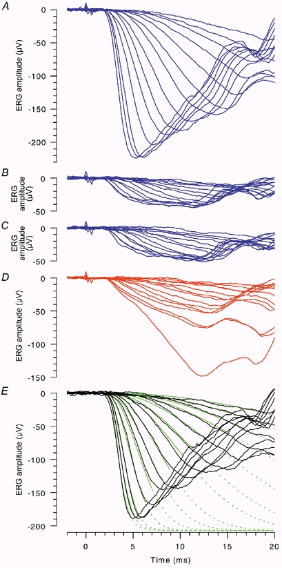
A family of dark-adapted responses to blue flashes (A) is predominantly of rod origin, but additionally contains input of cone origin. The ‘cone’ component for the same series of flashes is investigated in B-D, and the calculated rod-isolated response family is plotted in E. In each panel the same set of flash durations was used, ranging from 35 to 700 μs, and the subject's mean pupil diameter was 7.5 mm. A, ‘rod + cone’ responses. Blue flashes were presented in darkness, with sufficient intervals to allow full recovery of the rod response; the blue flashes delivered 34, 57, 87, 130, 230, 390, 600, 1200, 2000, 3600, 7200, 17 000, 29 000, and 62 000 Td s. B, the same blue flashes were delivered in the presence of a steady blue background of 1500 Td that saturated the rods, at intervals sufficient to allow recovery of the cone response. C, the same blue flashes were presented 1 s after an intense blue flash of 29 000 Td s; i.e. within the period of rod saturation (see Fig. 3). D, red flashes were presented in darkness; the photopic intensity of these red flashes was matched to that of the blue flashes, by use of a neutral density filter in conjunction with the red filter. The photopic intensity of the blue flashes was ca 1/11 of their scotopic intensity, while the scotopic intensity of the matched red flashes was ca 1/83 that of the blue flashes. Thus the brightest red flash delivered ca 6000 photopic Td s, and ca 750 scotopic Td s; it should have elicited ca 6400 isomerizations rod⁻¹ compared with ca 550 000 isomerizations rod⁻¹ for the brightest blue flash. Traces in A-D were averaged from 2-10 trials. E, rod-isolated response family, calculated by subtracting the ‘cone’ responses in C from the ‘rod + cone’ responses in A. Green curves plot the predictions of the model of phototransduction in eqns (3)–(4), fitted as an ensemble to the rod-isolated responses, using the measured flash intensities; these curves are shown as continuous over the intervals of fitting, and are continued broken thereafter. The parameters used were: maximal response, a_max= −207 μV; pure delay, t_d= 1.75 ms; membrane time constant, τ= 0.7 ms. With these parameters, the amplification constant obtained from the ensemble fitting was A= 3.9 s⁻², when the troland conversion factor was taken as K= 8.6 photoisomerizations rod⁻¹ Td⁻¹ s⁻¹.

Figure 11. Comparison of human rod responses obtained from paired-flash ERGs and from suction pipette recordings, under dark-adapted and light-adapted conditions.

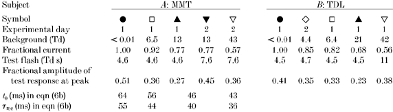
A, rod responses derived with the paired-flash technique for subject TDL. Results from Fig. 10B have been replotted on a slower time base, and for comparison with the suction pipette recordings have been normalized with respect to the dark current, i.e. the ordinate plots the fraction of dark current suppressed per photoisomerization (compare Fig. 9A). On the basis of a troland conversion factor of K= 8.6 photoisomerizations rod⁻¹ Td⁻¹ s⁻¹, the steady backgrounds delivered < 0.1, 46, 180 and 370 R* s⁻¹ (symbols as in Fig. 10B) B, data are from Kraft et al. (1993, Fig. 9), kindly supplied by Dr J. L. Schnapf, and are expressed in the same units as in A. For an assumed effective collecting area of 1.7 μm², the backgrounds were calculated to deliver 0, 14, 27, 51, 96, 230, 430 and 820 R* s⁻¹. Black traces indicate responses obtained on backgrounds that most closely matched those used in A. Curves in A show a model for rod responses suggested by Nikonov et al. (1998, eqn (19)), comprising the algebraic sum of three exponential decay terms. For the dark-adapted response, the three rate constants were set to 3.5, 25 and 50 s⁻¹. For responses on the three backgrounds, we scaled up each of these rate constants by a fixed factor, of 1.28 (at 46 R* s⁻¹), 1.42 (at 180 R* s⁻¹) and 1.7 (at 370 R* s⁻¹), and we scaled the amplitude of the responses in proportion to the fraction of steady current remaining on the background, i.e. we multiplied by 0.82, 0.68 and 0.56, respectively. In all cases the total delay term was t_d= 3 ms. The curves should be interpreted with caution, both because we needed to use an unusually high value for the amplification constant, of A= 19 s⁻² (cf. ≈4 s⁻² for the rising phase of the response, see Fig. 10), and because the formulation ignores calcium feedback mechanisms.

Light calibrations were performed using an IL-1700 photometer (International Light, Newburyport, MA, USA) with photopic (Y) and scotopic (revised Z-CIE) filters. Intensities will be given in scotopic units unless otherwise specified; i.e. corneal luminances will be in scotopic candela per square metre (cd m⁻²), and retinal illuminances in scotopic trolands (Td), where the troland is the unit of retinal illuminance given by the product of corneal luminance in cd m⁻² and pupil area in mm².

To calculate the flash intensity (Φ) in photoisomerizations per rod, we adopted the troland conversion factor K= 8.6 photoisomerizations rod⁻¹ Td⁻¹ s⁻¹ (Kraft et al. 1993; Breton et al. 1994). Thus we calculated:

(1)

where L is the integrated retinal illuminance of the flash (in Td s), given by the product of the integrated corneal luminance C (in cd m⁻² s) and the pupil area P (in mm²). The value adopted for K is not critical, as it simply scales the extracted estimate of amplification constant A (see next subsection). For brevity, we will usually ignore the fact that C and L are integrated over time, and refer to them simply as corneal luminance and retinal illuminance, respectively.

In a few experiments (Figs 6B, 7 and 10) we continuously presented an extremely dim blue background, which was barely visible to the dark-adapted subject. Our aim in doing this was to stabilize the adaptational state, and also to make it easier for the subject to remain alert. The intensity of this background was too low to measure with the photometer in its calibrated configuration, but from tests with and without the scotopic filter and radiometric lens in place, we estimate that it was around 0.0002 cd m⁻², corresponding to about 0.01 Td.

Figure 6. Extraction of the rod response at a continuum of measurement times.

A, rod-isolated responses to probe flashes presented either in darkness (heavier trace) or on steady backgrounds of 10, 27, 85, 150, 280 and 950 Td (bottom to top). The results are re-analysed from Fig. 2 of Thomas & Lamb (1999). Traces plot the response to a blue flash of 10 000 Td s (presented either in darkness or on a background), minus the response to a photopically matched red flash, presented on the brightest background to avoid rod intrusion at later times (compare Fig. 1D). B, ratio of the response from A obtained on each background to the response obtained in darkness. At early times, when the response is small, the ratio is susceptible to noise, and it has therefore not been plotted at times earlier than 2.4 ms. At times later than 15 ms (not shown) the ratio again becomes noisy. Within the window from 4 to 15 ms, however, the ratio is very nearly constant, indicating that the probe-flash response on each background is accurately described as a constant fraction of the dark-adapted probe response. C, rod-isolated responses to probe flashes of 8200 Td s, presented either alone (heavier trace) or at separations t_sep of 2, 5, 10, 15, 20, 40, 60, 80, 100,150, 200 and 400 ms after a test flash of 4.4 Td s. The smallest response was obtained at a separation of 100 ms (see Fig. 7). D, each of the probe flash responses from C, obtained following a test flash, has been divided by the response to the probe flash alone, to obtain the ‘fractional probe response’, R_sep(t_meas)/R_alone(t_meas). This ratio was noisy at early times, and again has only been plotted for times greater than 2.4 ms. Note the region from approximately 4-8 ms, over which the ratio is reasonably constant at each test-probe separation. Subject MMT; dilated pupil, 7.3 mm diameter. Inset: the range of measurement times, of 4.6-7.4 ms, shown in Fig. 7.

Figure 7. The a-wave and the derived rod response at a range of early measurement times.

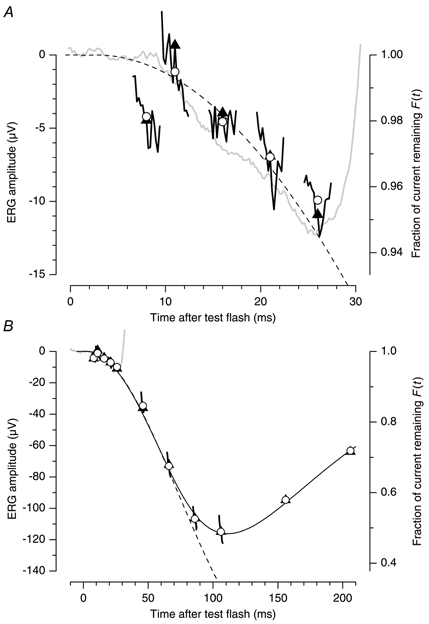
The ERG elicited by the test flash (grey trace) is compared with the rod response derived from the paired-flash results in Fig. 6. Each test-probe separation time, t_sep, in Fig. 6 leads to a ‘continuum’ trace for the derived rod response in this figure, where all measurements are plotted at the time after the test flash at which the probe response was measured, i.e. at t=t_sep+t_meas. These continuum traces are plotted over the window of measurement times t_meas from 4.6 to 7.4 ms, indicated by the inset in Fig. 6. ^, mean over this window; ▴, value at t_meas= 6 ms (i.e. at the centre of the window). The ordinate scale at the right plots the fractional probe response, exactly as in Fig. 6, i.e. F(t)=R_sep(t)/R_alone(t). The absolute scale at the left has been obtained as a_max(1 − F), where the maximal amplitude was obtained by fitting the family of a-wave responses, as a_max= −225 μV. The dashed trace plots the delayed Gaussian prediction of the model for pure activation, eqn (7a), with A= 5.4 s⁻², τ= 1 ms and t_d= 1.7 ms. The continuous trace plots eqn (6) using the same activation parameters, and t₀= 74 ms, τ_rec= 114 ms, and n = 8. A, expanded view at early times; B, full view, for measurements out to a test-flash separation of 200 ms. Additional details are given in legend to Fig. 6.

Figure 10. Derived rod sensitivities in darkness and on three backgrounds, for the other two subjects.

Derived sensitivities, obtained exactly as in Fig. 9B, are plotted for subjects MMT (A) and TDL (B). Parameters of the backgrounds, stimuli and fitted curves are tabulated below, for experiments on two days. While we were able to obtain an adequate fit for subject MMT (A) using the kinetics described in eqns (6b) and (7b), we were unable to fit the slower decline recorded for subject TDL (B) with the same equations; a fit using an alternative model is shown in Fig. 11. For subject MMT the fitted traces use A= 5.3 s⁻² and a total delay of t_d= 2.7 ms; in fitting families of dark-adapted responses we had found A= 5.1 and 5.3 s⁻² on the two days. For subject TDL the fitted traces use A= 4.3 s⁻² and a total delay of t_d= 2.7 ms; in fitting families of dark-adapted responses we had found A= 3.6 and 4.3 s⁻² on the two days. The symbols ⋄ for subject TDL plot the same points as in Fig. 5B.

Equation for the rising phase of the rod response

In the molecular description of Lamb & Pugh (1992), the fraction F of open cGMP-gated channels in the outer segment, at time t after a flash of Φ photoisomerizations, is given by:

(2)

where A is the amplification constant of transduction, and t_d is a delay term (which in practice combines delays both in the transduction machinery and in electrical filtering). The electrical current is predicted by convolving eqn (1) with an exponential decay (representing the rods’ membrane time constant, τ), an operation that can be performed analytically, to yield (for t≥ 0):

(3a)

where

(3b)

as derived in eqn (5) of Smith & Lamb (1997). The cell's response is the change in this circulating current from its resting level, given by:

(4)

RESULTS

Isolation of rod and cone signals

In attempting to record ERG signals from rods, a considerable problem arises from the fact that most stimuli also excite a cone response, and to obtain the ‘rod-isolated’ response it is necessary to obtain, and then subtract, an estimate of the cone contribution. Figure 1 shows a comparison of three standard approaches in the literature (e.g. Hood & Birch, 1990; Cideciyan & Jacobson, 1996). Figure 1A plots the ‘rod + cone’ responses obtained with a family of blue flashes, while Fig. 1B–D plots three estimates of the respective cone contributions. These were obtained: firstly (Fig. 1B), by delivering the same blue test flashes while the rods were saturated by a steady bright blue background; secondly (Fig. 1C), by delivering the same blue test flashes while the rods were transiently saturated shortly after an intense blue flash; and thirdly (Fig. 1D), by delivering red flashes of the same photopic intensity as the blue flashes (i.e. ‘photopically matched’ red flashes) under dark-adapted conditions. These red flashes are intended to stimulate the cones to the same extent that the blue flashes do, with minimal stimulation of the rods (but see next paragraph).

The responses in Fig. 1B and C are very similar to each other, suggesting that the two methods of inducing rod saturation (during a steady background, or following a bright flash) are broadly equivalent. The responses in Fig. 1D, however, differ from those in Fig. 1B and C at higher intensities, almost certainly because of a degree of rod excitation elicited by the red flashes (see below). Accordingly we chose not to use the photopic matching method, and instead we used the method of transient rod saturation after a pre-flash for our main experiments. The rod-isolated response family, obtained by subtraction of the estimated photopic contribution in Fig. 1C, is plotted in Fig. 1E. Over their rising phase these responses are well described by the family of responses predicted by the ‘activation only’ model of phototransduction given above in eqns (3)-(4). For this subject, the estimated maximal response was a_max= −207 μV, and the amplification constant required in fitting the family was A= 3.9 s⁻².

If we were to employ the method of rod saturation by steady light (Fig. 1B), we would need to show that the rods were fully saturated and that the cones were not desensitized. With regard to the second point, the steady blue background used in Fig. 1B is expected to cause negligible suppression of circulating current (Paupoo et al. 2000; Fig. 2) as well as negligible reduction in the rising phase of the response. From the work of Schnapf et al. (1990, p. 696) the photopic intensity of this light (ca 140 photopic Td) was more than a factor of 10 dimmer than the intensity needed to halve the sensitivity of monkey cones (around 2000 photopic Td), and so it seems most unlikely that it would cause any desensitization of human cones.

Figure 2. Amplitude versus flash intensity, for rod-isolated responses at fixed times.

A, the rod-isolated a-wave responses a(L, t) from Fig. 1E have been measured at a series of times, t, and plotted against flash intensity, L, in Td s. The measurement times were: t= 3 (^), 3.5 (□), 4 (Δ), 4.5 (♦), 5 (▿), 5.5 (★), 6 (□), 6.5 (▴), 7 (⋄), 8 (▾), 9 (⋆) and 10 (•) ms after the flash. B, the responses from A have been normalized to the maximal amplitude of a_max= −207 μV used in fitting Fig. 1E. Then, for each measurement time, the points have been shifted horizontally to provide the best alignment (by the least-squares criterion) to the exponential saturation function, eqn (5), shown by the continuous curve. This fitting was done using only those points connected by continuous lines, i.e. up to about the inflection point for each set. The horizontal scaling factors, −log₁₀k(t) in eqn (5), obtained by the fitting, were 5.19, 4.78, 4.48, 4.22, 4.01, 3.85, 3.72, 3.61, 3.47, 3.30, 3.12 and 2.99 log Td s. In each case k(t) was within 0.11 log₁₀ units of the predicted scaling factors given by eqn (2) as 1/2KA(t − t_d)², where the values of K, A and t_d are given in the legend to Fig. 1.

Likewise, in order to justify use of the transient rod saturation method (Fig. 1C), we require two controls: we need to show firstly that the rods remain fully saturated, and secondly that the cones are fully recovered, at the time of presentation of the test flashes. These criteria are investigated subsequently in Fig. 3, where we examine the effects of varying the interval between intense flashes. However, for the time being, we can say that the close similarity between the two families of responses (in Fig. 1B and C) suggests that each of them provides a true indication of the cone response elicited by the blue test flashes.

Figure 3. Recovery of the response amplitude for the second in a pair of bright flashes.

Pairs of identical bright blue flashes (200 μs duration, 190 cd m⁻² s), used subsequently as probe flashes, were delivered at a range of inter-flash intervals. Symbols plot the average response amplitude for the second flash, as a fraction of the average response amplitude for single flashes under fully dark-adapted conditions, at a measurement time of 6.5 ms. Filled symbols are for flash pairs delivered in darkness; open symbols for flash pairs on a steady background. A and B, subject TDL: mean pupil diameter 7.5 mm; flashes delivered 8200 Td s. Symbols: □, ▴, in darkness, on two days; ▵, on a blue background of 1 cd m⁻² (44 Td) on the second of these days. C and D, subject CF: mean pupil diameter 8.6 mm; flashes delivered 11 000 Td s. Symbols: □, •, ▴, in darkness, on three days; ▵, ▿, on blue backgrounds of 0.77 and 9.0 cd m⁻² (42 and 490 Td) on the third of these days. The right-hand panels show the same results as the left panels, but on a faster time scale and an enlarged vertical scale. Typically, each point was derived from four flash pairs, delivered at intervals of 60 s. However, for the measurements on backgrounds in C and D, the repetition interval was reduced to 45 or 30 s for flash separations shorter than 30 s. The curves plot the sum of assumed photopic and scotopic components, each representing the fading of an equivalent background light, as specified by the expressions in eqns (8) and (12) of Thomas & Lamb (1999); in addition, for experiments conducted in the presence of background illumination, we added the real light. For the photopic recovery, the time constant was 0.1 s for both subjects, and the amplitude of the component was 0.18 (TDL) and 0.19 (CF) of the total signal. For the rod recovery, we obtained an improved fit to the slow ‘tail’ phase by employing two components of fading equivalent background. We set the time constant of the dominant component to 0.5 s for both subjects, and we used a time constant of 2.6-5.8 s for the smaller tail component in the different adaptational conditions and subjects.

It is not surprising that a component of rod response is apparent in Fig. 1D. Measurement of the intensity of the red flashes showed that, in scotopic terms, they were only about 83 times dimmer than the corresponding blue flashes (see Fig. 1 legend), and therefore they would be expected to elicit a significant degree of rod excitation.

Response-intensity relation for the rod-isolated signal

Figure 2 focuses on the relationship between flash intensity and rod response amplitude. The rod-isolated responses in Fig. 1E were measured at a series of times from 3 to 10 ms, and the amplitudes have been plotted as a function of flash intensity in Fig. 2A. At any given measurement time (denoted by a given symbol) the response amplitude begins increasing with flash intensity, and at successive measurement times a given response amplitude is obtained at lower intensities, so that the response-intensity relations in Fig. 2A shift successively leftwards. At the very earliest measurement times (e.g. open circles, 3 ms; filled squares, 3.5 ms) the rise is likely to have been limited by the cell's capacitive time constant, and even an infinitely bright flash would not have elicited a maximal response.

Equations (2) and (4) predict that the shape of the response-intensity function measured at a fixed time should be described by the exponential saturation function:

(5)

where a(L, t) is the amplitude of the a-wave measured at time t after a flash of illuminance L, a_max is the maximal response used in fitting the family in Fig. 1E, and k(t) is a scaling factor that depends on the measurement time, t. Note that, for tractability, this equation has been derived using eqn (2), rather than the more complicated form in eqn (3); it therefore neglects the cell's capacitive time constant, and so is not expected to be applicable at the very earliest times.

In order to test whether eqn (5) provides a good description of the results, we calculated the best-fitting value of the intensity scaling factor k(t) for each measurement time, using a least-squares algorithm (fmin, Matlab) that we applied only for amplitudes up to the inflection point in each set, i.e. for those points joined by continuous lines in Fig. 2A. Figure 2B plots the results, after shifting the points according to the fitted k(t). It may be seen that the simple exponential saturation function provides a good description of the response-intensity relation at fixed times, for responses up to at least half-maximal. The fitted shift factors, −log₁₀k(t), are given in the legend, and in each case k(t) was close to the value of 1/2KA(t − t_d)² predicted by eqn (2).

Choice of probe flash intensity

The ideal probe flash would be one that was bright enough to drive the rod circulating current rapidly to zero before any post-receptoral signal set in, yet dim enough that the rods could recover fully within a reasonably short interval. However, from our fitting of the model curves in Fig. 1E, it appears that the first of these criteria cannot strictly be met, because none of the traces actually reach the fitted level of zero current before intrusion of the b-wave occurs. On the other hand, Fig. 1E suggests that each of the experimental traces obtained with a bright flash follows the predicted behaviour until shortly before its peak. Accordingly, measurements made with any of these bright flashes, at a time before the peak, ought to provide an amplitude representing a fixed fraction of the maximal response, and so it ought not to be critical what intensity of probe stimulus is chosen. Thus, Pepperberg et al. (1997) reported that the derived response was only weakly dependent on probe flash intensity, for intensities ranging from 2500 to 24 000 scotopic Td s, when delivered at the time of approximately two-thirds recovery following a just-saturating flash. Similarly, we have found that probe flashes ranging from 1300 to 33 000 Td s give closely similar estimates, when delivered 150 ms after a test flash of 5 Td s (i.e. at a range of probe-flash intensities, for the points at a separation of 150 ms in Fig. 8B); data not shown.

Figure 8. Reproducibility of measurements obtained on different days.

Rod responses for subject MMT, for a blue test flash delivering 0.13 cd m⁻² s (≈6.0 Td s). The experiment was repeated on three days over a period of 6 weeks. A, derived rod response, plotted as in Fig. 7B over the measurement window from 4.6-7.4 ms (as indicated by the inset in Fig. 6B). The first and third sets of results have been offset vertically for clarity. B, normalized rod response, expressed as a fraction of a_max. Each point has been obtained by averaging the fractional responses from A, over the measurement window (without the offsets), and the error bars indicate ± 2 s.e.m. In both panels, the continuous noisy curves at early times plot the ERG elicited by the test flash. Two forms of kinetic equation are illustrated in B. The decay term specified in eqn (6b) has been combined with either the Gaussian or the parabolic onset formulation of eqn (7a) or (7b). The Gaussian approach is illustrated by the dashed curve for Rise(t) (eqn (7a), using A= 6.5 s⁻²), by the dotted curve for Fall(t) (eqn (6b), using t₀= 72 ms, τ_rec= 120 ms), and by the continuous black curve for their product (eqn (6a)). For the parabolic formulation, we illustrate only the product, indicated by the grey trace (using A= 4.8 s⁻² as found in fitting the a-wave response family, t₀= 70 ms, and τ_rec= 48 ms). In all cases the total delay time was set to t_d= 2.7 ms, and the exponent in eqn (6b) was n = 8. All probe flashes delivered 190 cd m⁻² s (≈9000 Td s). In these early experiments we were unable to deliver probe flashes at separations of less than 60 ms, because we had only a single flash gun, and it could not trigger a second flash at shorter intervals.

Although a more intense probe flash has the advantage of saturating the response more rapidly, it has the disadvantage that a greater time is required for recovery, before the next flash can be delivered. As a compromise, we chose as our standard probe flash the fourth highest flash intensity in Fig. 1, i.e. a 200 μs duration blue flash, delivering 160-190 cd m⁻² s, corresponding to ca 7000-9000 Td s depending on pupil size. For comparison, Pepperberg et al. (1997) used 12 000-16 000 Td s, while Pepperberg et al. (2000) suggested the use of at least 10 000 Td s. In our initial analysis we chose to measure these probe responses at 6.5 ms, but, as we show subsequently, it turns out that the precise measurement time is not at all critical.

Recovery from probe flash: choice of stimulus repetition interval

We next determined the length of time required for recovery of the cones and rods following delivery of the probe flash. To do this, we presented pairs of our standard probe flashes, at intervals ranging from < 1 to 60 s, and examined the relative size of the second response as a function of the interval between the two identical flashes. To allow full recovery, we always waited at least 60 s before delivering a subsequent pair; tests with inter-flash intervals of 75 and 120 s (not illustrated) indicated that no significant additional recovery occurred later than 60 s.

The time course of recovery as a function of inter-flash interval is plotted in Fig. 3, for two subjects (TDL, upper row; CF, lower row). Each point plots the amplitude of the second response in the pair, as a fraction of the amplitude of the dark-adapted probe response. For pairs of flashes delivered in darkness (filled symbols), this was obtained simply as the amplitude ratio of the second flash response to first flash response (both measured at 6.5 ms). But for pairs of flashes delivered on steady blue backgrounds (open symbols), when the amplitude of the dark-adapted response was not simultaneously available, the amplitude ratio of second to first response was scaled by the mean ratio of light-adapted to dark-adapted probe response amplitude, obtained with probe flashes presented at long separations. In the left column (Fig. 3A and C), the recovery of normalized response is plotted on a slow time scale, while in the right column (Fig. 3B and D) the early part of these results is shown in an expanded view.

The recovery for both subjects is very similar, with an initial rapid but small component followed by slower complete recovery. At the very earliest separations (80 ms for TDL and 65 ms for CF) no response was obtainable, indicating saturation of both the cone and rod systems. One component of the response recovered rapidly, reaching a plateau of 18-20 % of the maximal ‘rod + cone’ level after about 0.4 s, and we interpret this to reflect recovery of the ‘cone’ component of the ERG. A second component of recovery began subsequently (after about 3 s for TDL, and about 1 s for CF), and reached the final level after 20-30 s for flashes delivered in darkness. This second component has all the hallmarks of the rod photoreceptor circulating current, setting in more rapidly but reaching a smaller level in the presence of blue backgrounds (open symbols). Curves are drawn in Fig. 3 that assume separate recovery of the cone and rod circulating currents. The equations used (see Fig. 3 legend for details) are based on the notion that the cone and rod systems each experience an ‘equivalent background’ light that fades with time; however, we do not attach great significance to the particular fits.

Our first conclusion from the experiments of Fig. 3 is that the repetition interval following our standard probe flash should be at least 20 s for flashes delivered in darkness, and at least 15 s for flashes delivered on a background that halves the rod circulating current. To err on the side of caution we adopted an interval of at least 30 s for experiments done in the absence of a background, and at least 20 s for those done in the presence of a background. Our second conclusion is that following a flash of this intensity there exists an interval, from about 0.5 s to at least 1 s (or even 3 s in subject TDL), during which the cone system is fully recovered, yet the rods remain fully saturated (see Elenius, 1967, 1969; Birch et al. 1995; Hood et al. 1996).

Accordingly, in all subsequent experiments, we determined the rod-isolated response by presenting stimuli during this interval of transient rod saturation. The signals obtained with stimuli delivered approximately 1 s after an intense flash (of the same intensity as the probe flash) were taken to originate in the cone system, and were subtracted from the signals obtained with identical stimuli delivered under fully recovered conditions, to yield rod-isolated responses. Typical traces obtained using this approach are illustrated in Fig. 1C and Fig. 4B.

Figure 4. Example of the paired-flash protocol.

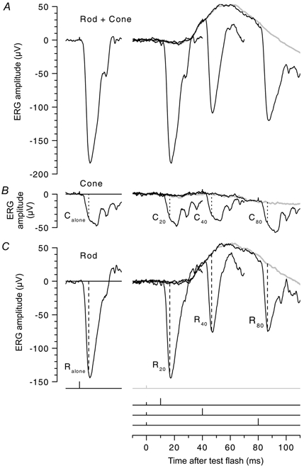
The left column shows responses to a bright blue probe flash (7200 Td s) alone, while the right column shows responses to a dim blue test flash (4.7 Td s) either alone (grey traces), or followed by the probe flash after an interval of 10, 40 or 80 ms. The small and large markers in the inset at the bottom show the timing of the test and probe flashes, respectively. A, raw ‘rod + cone’ responses, for test and probe flashes presented in the presence of a dim blue background (4.4 Td). B, ‘cone’ responses obtained with the same flashes presented during the period of transient rod saturation. The test and probe flashes were presented 1 s after a preceding flash of the same intensity as the probe flash, as in Fig. 1C; see also Fig. 3. C, ‘rod-isolated’ responses, obtained by subtraction of the traces in B from those in A. Dotted and dashed vertical lines, at t_meas= 6.5 ms after the probe flash, indicate the measured probe response amplitudes. The labels C₄₀ and R₄₀, etc., denote the cone and rod components of the probe flash response, for a separation time of t_sep= 40 ms between the test and probe flashes, while C_alone and R_alone denote the corresponding components in response to the probe flash alone. Subject TDL, pupil diameter 7.5 mm.

The paired-flash technique: extraction of the rod's response to a test flash

Figure 4 illustrates the application of the paired-flash technique, to derive the time course of the response to a blue test flash of 4.7 Td s; for the purposes of illustration, this experiment was performed in the presence of a steady background (4.4 Td). The timing of the test and probe flashes is indicated at the bottom of the figure by small and large markers, respectively. The left column shows responses to the probe flash alone, and the right column shows responses to the dim blue test flash, presented either alone (grey) or followed by the probe flash at one of three representative intervals. Figure 4A plots the raw ‘rod + cone’ responses, while the middle row (Fig. 4B) plots ‘cone’ responses obtained when the same flashes were presented during the period of transient rod saturation elicited by an intense flash (approximately 1 s after a flash of the same intensity as the probe flash, as described above). Finally, the bottom row (Fig. 4C) plots the rod-isolated signals obtained by subtracting the responses in Fig. 4B from those in Fig. 4A.

The rod-isolated response to the test flash alone (Fig. 4C, right, grey trace) is almost flat for the first 25 ms; thus the a-wave, representing the photoreceptor response, is negligibly small. At later times the response is dominated by the positive-going b-wave, which peaks at around 60 ms, and which originates from post-receptoral activity. The purpose of presenting the probe flashes is to expose the photoreceptor response hidden beneath this post-receptoral activity: the idea is that the bright flash will rapidly eliminate the photoreceptor current, but that initially the post-receptoral signal will be unaltered.

Examination of Fig. 4C shows that, for a probe flash delivered just 20 ms after the test flash there was little change in response amplitude. However, for probe flashes delivered at intervals of 40 or 80 ms after the test flash, the amplitude of the rod-isolated probe response (dashed vertical lines) was significantly smaller than the response to the probe flash alone. This reduction in probe response amplitude indicates that the rod circulating current was reduced for these later presentations.

In contrast, the responses in Fig. 4B indicate that the dim blue test flash had negligible effect on the cone system. Thus, the cone a-wave and b-wave were both small, and the responses to the probe flashes at all test-probe separations were very similar, both in size (vertical dotted lines) and in shape, even including the oscillatory potentials.

Figure 5 illustrates the way that the probe-flash measurements from Fig. 4B and C can be used to derive the time course of the response to the test flash, for both the rod and cone systems. We begin by mentioning two conflicting considerations that influence the time at which we should measure, after the probe flash. On the one hand, the measurement time should be as early as possible, in order to minimize any change in post-receptoral response elicited by the probe flash, in comparison with the post-receptoral response to the test flash alone. On the other hand, the measurement time should be late enough after the probe flash to permit the photoreceptor circulating current to have fallen to zero. As a compromise, we chose a measurement time just before the peak of the response, at t_meas= 6.5 ms.

Figure 5. Extraction of the underlying rod and cone components of the response to a test flash.

Analysis of paired-flash experiment, using the results in Fig. 4 for illustration. The assumption of this analysis is that at the measurement time (6.5 ms after the probe flash), the amplitude of the probe response represents some fixed fraction of the photoreceptor circulating current at that time (see Fig. 1). Accordingly, by aligning the head of each arrow (C₄₀, R₄₀, etc.) at a common level (representing saturation), the base of the arrow should provide a measure proportional to the photoreceptor current. Hence the open symbols (^) and the filled symbols (•) plot the derived measures of cone and rod response, respectively. These were obtained from the representative responses in Fig. 4, together with responses for additional test-probe separations. For purposes of illustration, this experiment was performed in the presence of a steady blue background of 4.4 Td, and the ordinate scales are therefore plotted relative to that level, in units of microvolts on the left, and in normalized units on the right. A, the response of the cones (^) was unmeasurable for the blue background and blue test flash used here. B, for the rods (•), the derived flash response is labelled r(t), and the steady response is labelled r_steady; this latter level was derived by comparison with the dark-adapted probe response, R_DA (not illustrated in Fig. 4). The continuous trace plots the rod-isolated ERG recorded with the test flash alone, as in Fig. 4C, right.

If we were able to assume that, at the time of measurement, the post-receptoral response to the test flash was unchanged by presentation of the probe flash, then the difference between the traces (indicated by each vertical line) would represent the photoreceptor signal alone. If we could also assume that, by the time of measurement, the photoreceptor current in response to the probe flash had fallen to zero, then the length of each vertical line would represent the photoreceptor circulating current remaining at that time after the test flash. However, inspection of the fourth largest trace in Fig. 1E suggests that at a measurement time of 6.5 ms after the probe flash, the current is actually reduced to only about 20 % of its pre-existing level. As we shall show later, this means that, to a reasonable approximation, we can take the lengths of the vertical lines to represent a fixed fraction (ca 80 %) of the photoreceptor current present at the time of measurement. However, a proper analysis of this situation is quite complicated, and will be deferred until the Discussion.

We begin in Fig. 5B by plotting the rod-isolated probe-alone amplitude (R_alone, from Fig. 4B) as the downward arrow, from the reference level which is defined as zero during the steady state (dim blue background). On the basis of the two assumptions above, the head of R_alone represents the saturated level of photoreceptor response, and accordingly we have aligned the heads of all the other probe response arrows at the same level. For example, the arrow R_DA at the left plots the amplitude of a probe response recorded in fully dark-adapted conditions (not illustrated in Fig. 4). Its upper end provides a measure of the rod circulating current in darkness, and hence the size of the steady rod response r_steady elicited by the background is indicated by the difference between R_DA and R_alone.

In the same way, the upper end of the arrow labelled R₄₀ gives a measure of the rod response amplitude for a test-probe separation of 40 ms, and similarly for all the other separations tested. Each point is plotted at the time of measurement relative to the test flash, i.e. at t=t_sep+t_meas, as employed by Hetling & Pepperberg (1999), and as will be explained more fully in the Discussion.

Rod-isolated measurements are indicated by the filled circles which, for the different separations, plot r(t_sep+t_meas) =R_alone − R_sep (where R_sep is the response obtained at a separation of t_sep, e.g. R₄₀ at t_sep= 40 ms). The normalized scale on the right measures the fractional rod response, r(t)/r_max where r_max=R_alone, and represents the fractional suppression of circulating current in the rods. The scale of microvolts on the left is expected to slightly underestimate the absolute size of the photoreceptor response, because (as illustrated in Fig. 1E) measurement of the probe response amplitude at 6.5 ms yields only about 80 % of a_max; accordingly this scale should represent approximately 80 % of the true amplitude.

The rod response r(t) (filled circles) derived for this blue test flash reached peak in a little under 100 ms, at a level of about 30 % of maximal. For comparison, the rod-isolated ERG response to the same test flash is plotted as the continuous trace (this is an extension of the grey trace plotted previously in Fig. 4C, right). It can be seen that the paired-flash approach is able to extract the rod response at times when the photoreceptor component of the ERG was completely swamped by the b-wave.

Cone-isolated measurements are plotted as the open circles in Fig. 5A. The results confirm our impression, gained from visual inspection of Fig. 4B, that the blue background and blue test flash used in this experiment elicited no detectable cone component of steady response or of flash response.

In all our experiments with paired flashes, we presented the test-plus-probe combination at least six times at each stimulus separation. As a result, the plotted responses are typically averaged from six trials (though on some occasions more trials were presented, and in a few cases some trials were rejected because of noise).

Since the recovery interval between stimuli was usually 30 s, the time taken to accumulate one group of paired-flash responses at the 10 different test-probe intervals (as well as test-alone and probe-alone responses) was typically around 8 min. Thus, for six repetitions of the procedure, it took at least 50 min of stable ERG recording to obtain a single set of measurements of the kind illustrated in Fig. 5.

Measurement of probe response at a continuum of times

One of the uncertainties in the analysis up to this stage has been in knowing how to select the most appropriate time at which to measure the probe responses. For our standard 200 μs duration probe flash (ca 160-190 cd m⁻² s, or ca 7000-9000 Td s) that reaches peak in about 7 ms, we chose in the preceding analysis to measure the amplitude at t_meas= 6.5 ms, just before the time to peak (see Fig. 1E). Recently, Hetling & Pepperberg (1999) reported that their results were not greatly affected by whether they measured at 5, 6 or 7 ms. However, there appears to be no compelling reason for choosing any particular one of these values, and therefore we decided to investigate the consequences of altering the time of measurement.

Before applying this approach to the paired-flash technique, we first applied it to probe flashes delivered in the presence of steady backgrounds. Figure 6a shows responses to a probe flash of constant intensity, presented either in darkness (bold trace) or in the presence of backgrounds of progressively higher intensity. As reported by Hood & Birch (1993) and Thomas & Lamb (1999), the maximal response amplitude (a_max) declines as a function of increasing intensity. Those authors also reported that the amplification constant (A) of the rising phase was essentially unaltered by background illumination, so that the rising phase of each response should simply scale in amplitude. We have tested that prediction in Fig. 6B, by dividing each probe response by the dark-adapted probe response (bold trace in Fig. 6A). Apart from very early times, before a substantial amplitude had developed (< ca 4 ms), each probe response is very nearly a constant fraction of the dark-adapted probe response. Thus, for each background intensity, the entire probe response (from 4-15 ms) is simply a scaled version of the dark-adapted response. Hence, in the case of steady background illumination, the time of measurement of the probe response has negligible effect on the estimate of fractional suppression of current.

The results of a comparable analysis are illustrated in Fig. 6C and D, for probe flashes presented at a range of intervals following a given test flash, i.e. for an experiment similar to that in Fig. 4C. For the raw responses in Fig. 6C, the bold trace denotes the probe-alone response, while the smallest response was obtained for a separation time of t_sep= 100 ms. As pointed out by Pepperberg et al. (1997), all the responses have quite similar kinetics, and in particular they exhibit a consistent time to peak, of about 6.5 ms for this subject. In Fig. 6D, each test-plus-probe response has been divided by the probe-alone response. Thus, for each test-probe separation t_sep we have plotted a trace over a range of measurement times, t_meas, giving the ‘fractional probe response’, defined as R_sep(t_meas)/R_alone(t_meas).

As in the case with steady background illumination, the ratio exhibits a fairly flat region for a range of measurement times, although here the flat range in most cases extends only from about 4-8 ms. At earlier times the ratio is poorly defined, presumably because of noise in the small probe-alone response, while at later times the ratio appears to vary systematically from the approximately constant value obtained up until about 8 ms. For four of the test-probe intervals, though, the ratio exhibited an appreciable downward slope during the window of 4-8 ms after the probe flash. In fact, we would expect a finite slope on many of the traces, because of the changing rod response, i.e. from the slope of the rod's response to the test flash, which is downwards before the peak and upwards after the peak. From the subsequent results in Fig. 7, the slope of the extracted response for this test flash intensity has a maximal slope during the rising phase of about −1.7 μV ms⁻¹, or around −0.007 ms⁻¹ in fractional terms. However, the maximal downward slope seen in Fig. 6B is about three times as large, at −0.02 ms⁻¹, while no appreciable upward slope is apparent in any of the traces. One possible contributory factor to an apparent slope might be an earlier onset of post-receptoral signals. But in any case, the finding that the fractional response traces are reasonably close to constant over the window of about 4-8 ms suggests that the precise time of measurement ought not to be critical in determining the response to the test flash, although it may have some effect. Furthermore, it may be possible to reduce the level of noise in the analysis by averaging the calculations over a suitable period within this window.

Comparison between the rod responses derived by the two approaches, and with the rise of the a-wave

From the results shown in Fig. 6C and D, the derived rod response is plotted in Fig. 7 using two approaches, (1) measurement at a fixed time, and (2) measurement over a window of time. For each test-probe separation interval, t_sep (that is, for each trace in Fig. 6C and D), Fig. 7 contains filled triangles, plotting the response derived at a fixed measurement time of t_meas= 6 ms, together with a noisy trace, plotting the response derived over the time window from 4.6 to 7.4 ms indicated by the inset in Fig. 6D; in addition, the mean obtained over that window is shown by the open circles.

As in Fig. 5, the results have been plotted at the time at which the measurements were made, i.e. at t=t_sep+t_meas relative to the test flash. To obtain the left-hand vertical scale in absolute units of microvolts, we have simply multiplied the change in fractional scale on the right by the maximal a-wave amplitude, a_max, i.e. the left-hand scale plots (1 − F) a_max. For this subject, the maximal a-wave amplitude, obtained in fitting a response family of the kind illustrated in Fig. 1E, was a_max= −225 μV. This procedure of scaling of the fractional response (R_sep/R_alone) by the amplitude a_max is exactly equivalent to scaling the raw responses R_sep by the factor a_max/R_alone, and it corrects the absolute values for the effect mentioned in relation to Fig. 5 whereby measurement of the probe response amplitude at 6.5 ms records only about 80 % of the saturating level (i.e. R_alone/a_max≈ 0.8).

In the greatly expanded view of the early rising phase presented in Fig. 7A, the traces appear quite noisy. However, the absolute level of this noise is only a few microvolts, and can be seen to be relatively small in comparison with the full range of the response plotted in Fig. 7B. Note that all the measurements in Fig. 7A (centred at 8, 11, 16, 21 and 26 ms) appear as the first five pairs of symbols in Fig. 7B, where the open symbols almost obscure the filled symbols.

The continuum approach is useful in two ways in the expanded time scale of Fig. 7A. Firstly, it demonstrates that the precise time of measurements (t_meas) is not very critical, and can even be later than the peak of the probe response without degrading the derived rod response. Secondly, it shows that the time course of the derived response conforms closely to the rising phase (a-wave) of the ERG response to the test flash (continuous grey trace in Fig. 7). However, we would emphasize that the vertical correspondence between the ERG trace and the derived measurements depends critically on the amplitude of the probe-alone response, with which all test-plus-probe responses are compared; if the amplitude of the probe-alone response happened for any reason to be in error by a few microvolts, then all the derived values would be displaced by that amount. Hence it is critical for such a comparison to ensure that the measurements at small test-probe separations are carefully interleaved with probe-alone measurements.

In Fig. 7B we can examine the behaviour at longer times, and the measurements up to about 80 ms again appear consistent with our expectations for the shape of the rising phase. Thus, the points fall very close to the prediction (dashed curve) for the pure activation model of eqn (2), with the same amplification constant of A= 5.3 s⁻² that had been used in fitting the family of a-wave responses of the type illustrated in Fig. 1E. The continuous curve plots an equation we describe later that provides an empirical description of the response recovery.

Our interpretation of the results of Fig. 7 is that they provide several controls. Firstly they show that, over the early rising phase of the rod response (Fig. 7A), the paired-flash protocol extracts a response that (within the constraints of noise) is closely similar to the rod response reflected directly in the a-wave of the ERG. Secondly they show that over the later region of the rising phase (Fig. 7B) the derived measurements follow fairly closely the predictions of the pure activation theory. Thirdly, as reported by Hetling & Pepperberg (1999), the results of Fig. 7 show that the time of measurement does not appear to be particularly critical. Nevertheless, a number of the continuum plots exhibited quite a steep slope, indicating that the derived time course is to some extent dependent on measurement time. One possibility would be that this results from some kind of dependence of the post-receptoral response to the probe flash on the level of response to the test flash. If this were the case, then the response derived at the earliest possible measurement time would be expected to be least affected by such a phenomenon; however, it would also be based on the smallest response, and therefore most subject to noise. A second possibility is that we might not be measuring a constant fraction of the total current, with probe flashes presented during the responses to test flashes.

As a compromise between the three conflicting objectives of (i) measuring at very early times, (ii) obtaining a large response and (iii) averaging over a broad window, we chose to employ the continuum method, averaging over the window 6 ± 1.4 ms indicated by the bar in the inset to Fig. 6D.

Reproducibility of responses measured on different days

In Fig. 8 we plot measurements of the derived rod response to a constant test stimulus, presented on three separate days over a period of 6 weeks. The measurements were derived using the continuum method illustrated in Fig. 6 and Fig. 7, and each noisy section of trace in Fig. 8A plots the fractional probe response determined for a particular test-probe separation interval, and is taken to represent the fractional rod current F(t) remaining after the test flash. The middle response (grey) is plotted at the correct vertical position, and the other two responses are displaced vertically by ± 0.2 for clarity. For comparison, the ERG response elicited by the test stimulus on each of the three days is plotted as well, normalized according to the maximal amplitude, a_max, in order to provide an estimate of fractional circulating current. In these early experiments we had only a single flash gun, which meant that the inter-flash interval could not be reduced below 60 ms, so we do not have derived measurements that overlap in time with the a-wave of the ERG.

In Fig. 8B the results for the three experiments are superimposed and inverted, to plot the fractional response R(t)= 1 − F(t). In this panel we have plotted the means calculated over the window of 6 ± 1.4 ms, as described in Fig. 6 and Fig. 7, with error bars of ± 2 s.e.m. These results indicate that the recordings were stable over an extended period, and that the paired-flash protocol gave quite similar estimates of response amplitude and kinetics on different days, with a time to peak of around 100 ms for a response of ca 60 % maximal.

Kinetics at later times

The results of Fig. 7 confirm the findings of Pepperberg et al. (1997) that the rising phase of the response extracted by the paired-flash technique is closely similar to that predicted by a continuation of the theoretical curves fitted to the a-wave responses, and we now consider even later times. For many years, the kinetics of photoreceptor responses have been arbitrarily described in terms of a power-law rise followed by an exponential recovery (Baylor et al. 1974), using the equations tⁿ⁻¹exp(-t/τ) and other closely related forms to describe the dim-flash response (e.g. Hood & Birch, 1993; Pepperberg et al. 1997). Recently a modification of this approach was proposed by Hetling & Pepperberg (1999), who used the pure activation equation of the Lamb & Pugh (1992) model, multiplied by an exponential decay with an appropriate time constant.

When we used this same approach, we found (as reported by Hetling & Pepperberg, 1999) that we needed to assign a considerably higher value of amplification constant A than had been used in fitting the family of responses (cf. Fig. 1E); this presumably reflects the fact that the exponential term has already decayed considerably during the rising phase of the response. To avoid this problem, we adopted a decay term that is essentially unity at early times, but that then declines exponentially at later times. The form that we chose is plotted in Fig. 8B as the dotted curve, and is specified by the equation:

(6a)

with:

(6b)

where n, t₀ and τ_rec are constants; see Fig. 8 legend. To describe the rising phase in Fig. 8B we used two formulations, either the Gaussian expression from eqns (2) and (4), or its small-signal parabolic approximation, as follows (in both cases for t > t_d):

(7a)

(7b)

Note that the latter form of kinetics, combining eqn (7b) with eqn (6), is closely analogous to the ‘Poisson’ expression, tⁿ⁻¹exp(-t/τ), employed by Baylor et al. (1974), when the number of ‘stages’ in their formulation is given by n = 3.

The Gaussian rising phase of eqn (7a) is illustrated by the dashed curve in Fig. 8B, and the product given by eqn (6) is plotted as the continuous black curve, which provides a fair description of the measurements. However, a major difficulty with this approach of multiplying the Gaussian rise by a decay term is that at late times Rise(t) in eqn (7a) approaches unity for all flashes, so that the recovery phases for bright flashes of different intensity are predicted to superimpose. An alternative approach is to obtain Rise(t) from the small-signal approximation in eqn (7b), which has the advantage that the predicted response is then linear with flash intensity; on the other hand, this predicted response has the shortcoming that it does not saturate with increasing flash intensity, as it is a strictly linear formulation. The predicted response obtained by this second approach, of combining eqn (7b) with (6), is illustrated by the grey trace in Fig. 8B. Again, the curve provides an adequate description of the measurements. For the Gaussian formulation of eqn (7a), the fitting of the dim-flash response required a value of amplification constant (A= 6.5 s⁻²) only slightly larger than had been required in fitting the family of a-wave responses (A= 4.8 s⁻²); for the parabolic formulation of eqn (7b), we were able to use exactly the same value of A (4.8 s⁻²) as previously. (The time constant of recovery, τ_rec, differed for the two traces, because eqn (7a) saturates, whereas eqn (7b) continues to rise; see legend.)

We would stress that we attribute no particular physical significance to the form of recovery specified in eqn (6). We have simply found that eqns (6) and (7) together provide a convenient means of describing the shape of the observed responses, and accordingly we have used them to describe the kinetics measured in Figs 7A and B, 8A and B, 9B and 10A.

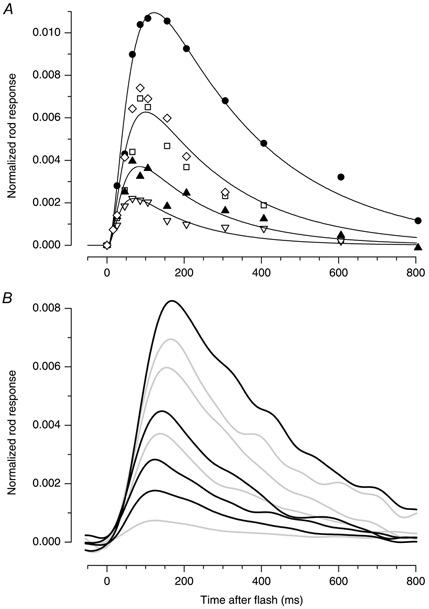
Figure 9. Derived rod sensitivities in darkness and on four backgrounds, for one subject.

A, the derived rod response for subject CF, obtained as in Figs 7 and 8, has been divided by test flash intensity to yield the response per unit intensity, in units of μV Td⁻¹ s⁻¹. B, these results have been further normalized with respect to the probe-alone response R_alone, to yield the fractional response per unit intensity, in units of Td⁻¹ s⁻¹. This normalization means that the response is expressed as the fractional suppression of the existing circulating current in the steady state. The experiment was performed over two days, with three of the backgrounds studied on both days; the background intensity, test intensity and peak response amplitude corresponding to the different symbols are tabulated below. Each point was obtained from typically six test-probe presentations, with the probe-alone response obtained from typically 10 flashes. As in Fig. 8B, the points have been averaged over a measurement window from 4.6 to 7.4 ms. In B the points for the middle three sets of data (♦, ▴, ▿) were calculated as the weighted means of the points plotted in A obtained on the two days, as indicated by the groupings tabulated below. The curves plotted in B are eqn (6) with the parabolic rise of eqn (7b), using A= 4.3 s⁻² (the average amplification constant found in fitting the a-wave families) and t_d= 2.7 ms, and with the decay parameters t₀ and τ_rec in eqn (6b) set as below, with n = 8.

Rod responses obtained in the presence of adapting background illumination

We next investigated the effect of background illumination on the rod photoreceptor response. Thus, for a given subject, we applied the paired-flash protocol to measure the rod response both in darkness and in the presence of a range of scotopic background intensities. Our aim in these experiments was to examine the rod response in the ‘small signal’ regime where the response is expected to be linearly dependent on flash intensity. However, because of the existence of noise in the measurements (see Fig. 7) it was in practice necessary to use a response of moderate amplitude, and we compromised by aiming for a peak response amplitude to the test flash of about 40 % of the maximum attainable on that background (see the right-hand ordinate scale in Fig. 5). Since it is well known that the sensitivity of the rod response decreases in the presence of background illumination, we increased the test flash intensity to generate a response of similar fractional amplitude when backgrounds were used.

Responses obtained under both dark-adapted and light-adapted conditions are plotted in Fig. 9 for subject CF. In Fig. 9A the derived responses have been divided by test flash intensity to provide the rods’ response per unit of flash intensity, in μV Td⁻¹ s⁻¹. The uppermost set of measurements (filled circles) was obtained in dark-adapted conditions, using test flashes of 3.3 Td s, while the other symbols were obtained for test flashes of 6.6-16 Td s presented in the presence of background illumination at four intensities (6.2, 15, 47 and 180 Td). The experiments were performed over two days, and measurements for three of the backgrounds were obtained on both days; see legend for details.

It is worth noting the long recording time needed to collect the results for this kind of experiment. For each of the five adaptational states (three of which were repeated on two occasions), we employed 10 or more test-probe separation intervals (plus the test alone, and the probe alone), and for each separation we presented at least six responses to the paired flashes (and at least 12 responses to probe flashes alone), delivered at intervals of at least 30 s in darkness or 20 s on backgrounds. As a result, collection of the data for the one subject in Fig. 9 took nearly 1 h per adaptational state, or a total of about 10 h of stable recording over the two days.

Sensitivity and fractional sensitivity

As argued recently by Pugh et al. (1999), one may examine the sensitivity of the underlying rod transduction mechanism (after exclusion of ‘response compression’) by plotting the sensitivity measurements normalized with respect to the remaining circulating current in the rods. This is equivalent to using the scale r(t)/r_max indicated schematically on the right of Fig. 5, but additionally with division by the test flash intensity to convert to ‘sensitivity’. The results of Fig. 9A are re-plotted in this form in Fig. 9B, on an ordinate scale of fractional response per unit intensity.

The inter-conversion between Fig. 9A and Fig. 9B according to circulating current has relatively little effect on the overall form of the responses, because the brightest background that we used suppressed only about half of the circulating dark current, i.e. reduced the probe-alone response to about 50 %. Thus, the points for the brightest background in Fig. 9B are roughly doubled in comparison with those in Fig. 9A, in relation to the dark-adapted points.

Corresponding results for the other two subjects (MMT and TDL) are plotted in Fig. 10, for darkness and three scotopic backgrounds, using the ordinate scale of fractional response per unit of flash intensity introduced in Fig. 9B.

Dark-adapted sensitivity and time to peak

The ‘sensitivity’ of the rod is conventionally defined as the peak response amplitude per unit of flash intensity (provided that the response is within the linear range that applies for relatively dim flashes); thus, the sensitivity in different adaptational conditions is given graphically by the peak of each of the traces in Fig. 9A. For the corresponding traces in Fig. 9B, we employ the term ‘fractional sensitivity’ to denote the peak of each trace when plotted on a scale of fractional response per unit intensity (as introduced by Nikonov et al. 2000).

Under dark-adapted conditions, the time to peak was approximately 120 ms and the fractional sensitivity was around 0.1 Td⁻¹ s⁻¹, for each of the three subjects. On the basis that the troland conversion factor is K= 8.6 photoisomerizations rod⁻¹ Td⁻¹ s⁻¹, this would correspond to a fractional sensitivity of about 0.01 photoisomerization⁻¹, indicating that at the peak of the rod's response a single photoisomerization suppresses approximately 1 % of the circulating current under dark-adapted conditions. As we shall see in Discussion, these values for time to peak and sensitivity are broadly in line with previous measurements, although they are marginally faster and less sensitive than those obtained in most single-cell recordings from mammalian rods.

Light-adapted response kinetics

The results illustrated for the three subjects in Fig. 9 and Fig. 10 are closely similar, and each displays the classic hallmarks of photoreceptor light adaptation. Thus, in the presence of background illumination the time to peak shortens and the sensitivity declines, consistent with the idea that recovery sets in earlier, and furthermore these changes are graded with the background intensity. In going from dark-adapted conditions to a background of ca 50 Td for each subject, the time to peak declined from ca 120 to ca 75 ms, and the fractional sensitivity declined to about 30-40 % (corresponding to a decline in the absolute sensitivity, shown only for subject CF in Fig. 9A, to about 15-20 % of its dark-adapted level). In one subject (CF) tested at a higher background intensity the time to peak further declined to around 70 ms and the fractional sensitivity fell to around 20 % at ca 170 Td.

For each of the subjects it also appeared that the early rising phase of the fractional response was essentially unchanged, for the background intensities that we examined. Thus, the pure activation rising-phase parabola with a constant value of A (dashed trace in Fig. 9B and Fig. 10) appears equally applicable to the results in darkness and on backgrounds for each subject, within the experimental error associated with the points, as illustrated, for example, in Fig. 8B. This result is consistent with the reports by Hood & Birch (1993) and Thomas & Lamb (1999) that in the presence of backgrounds of this intensity range the a-wave response of the rod-isolated ERG can be described simply by a reduction in maximal response amplitude, without any significant change in amplification constant, A. Those a-wave measurements were, however, restricted to very early times in the response (ca 10 ms), whereas our present results extend the time of common rise of the fractional response to the order of 50 ms for dim backgrounds.

The different continuous traces plotted in the two panels (Fig. 9B and Fig. 10A) were obtained using eqn (6) with a constant value of A, together with progressively earlier ‘peeling-off’ of the recovery phase in the presence of brighter backgrounds. This was achieved by progressively reducing the value of the delay parameter t₀ that characterizes the onset of recovery, and also reducing the time constant τ_rec, in eqn (6b).

For subjects CF (Fig. 9B) and MMT (Fig. 10A), the curves obtained using eqns (6) and (7) generally provide an adequate description of the experimental points, although there is a hint of the existence of a slow tail of recovery at late times. For subject TDL (Fig. 10B) the recovery phase was slower than for the other two subjects, and the shape of the response appeared somewhat different. In this case we had difficulty in obtaining an adequate description of the results using eqns (6) and (7) but, as shown in the next section, we were able to obtain a reasonable fit with another equation.

Comparison of paired-flash ERG and suction pipette responses

We were intrigued to compare the responses obtained in vivo using the paired-flash technique with those recorded previously using the suction pipette technique with human rods from eye donors (Kraft et al. 1993). In Fig. 11A, the responses from Fig. 10B for subject TDL have been replotted on an extended time base and on an altered vertical scale, as the fraction of the original dark current suppressed per photoisomerization. Thus, the results from Fig. 10B have been multiplied by the fractional current in the presence of each background, and divided by the troland conversion factor, K= 8.6 photoisomerizations rod⁻¹ Td⁻¹ s⁻¹. In this form, our results are directly comparable to those presented by Kraft et al. (1993) in their Fig. 8, after similar conversion of the light intensity to photoisomerizations (from units of incident photons μm⁻²) using their estimated collecting area of 1.7 μm². Their results, scaled in this way, are replotted in Fig. 11B using data kindly supplied by Dr J. L. Schnapf. We have used black traces to denote those backgrounds in Fig. 11B that were closest in intensity to the ones we used in Fig. 11A, and grey traces for the remaining backgrounds.

Comparison of the two panels in Fig. 11 shows a remarkably close correspondence between the paired-flash ERG measurements and the single-cell suction pipette measurements, for the response kinetics and light-adaptation behaviour of human rod photoreceptors. Not only are the shapes of the dark-adapted and light-adapted responses similar in the two panels, but in addition the absolute scaling of sensitivity is very similar (compare vertical scales), as is the absolute scaling of background intensity required to desensitize the response. However, for each adaptational state, it appears that the time to peak of the response is somewhat earlier in Fig. 11A than in Fig. 11B.

To aid comparison between the two panels, we have drawn a set of curves in Fig. 11A. As we were unable to obtain an adequate fit at late times using the formulation in eqns (6) and (7), we instead used eqn (19) of the recent theoretical description by Nikonov et al. (1998). Details are given in the legend.

We chose to illustrate the results for subject TDL because his responses (in Fig. 10B) showed a closer correspondence to the single-cell recordings than did the responses for the other two subjects. As noted previously, the derived responses for CF and MMT (in Fig. 9 and Fig. 10A) recovered to baseline more quickly that those for TDL, but we have no satisfactory explanation for why this should be so. One contributory factor might be age (CF, 30; MMT, 33; TDL, 51 years), but this suggestion fails to explain the close similarity of waveform between TDL's responses and the single-cell recordings, as the latter were recorded in a rod from a deceased 3-month-old human infant (J. L. Schnapf, personal communication). It is possible that some of the difference between the results for CF and MMT and those from single-cell recordings might relate to isolation of the retina from the retinal pigment epithelium, a procedure which might substantially alter the extracellular environment of the outer segments, as well as disrupting retinoid traffic.

Steady current and flash sensitivity as functions of background intensity

In Fig. 12 we have plotted the measurements of steady circulating current and flash sensitivity obtained in the experiments of Fig. 9 and Fig. 10, and for several additional experiments. In all cases the measurements are plotted relative to the values obtained under dark-adapted conditions, to give relative circulating current (Fig. 12A), relative sensitivity (Fig. 12B), and relative fractional sensitivity (Fig. 12C). For the sensitivity measurements in Fig. 12B and C, we have only included measurements obtained using test flash intensities that gave responses smaller than 45 % of the maximal response obtainable on that background. This level was chosen to allow reasonably large responses to be obtained in the presence of the inevitable recording noise, while avoiding responses that were well out of the linear range. In addition, we have plotted (as open stars) measurements of fractional response and sensitivity reported by Pepperberg et al. (1997). They employed the paired-flash technique to record responses using a fixed interval of 170 ms between test and probe flashes, for test flashes at a range of intensities presented either in darkness or on backgrounds of three intensities. From their response-intensity measurements, they obtained a sensitivity parameter (k, see legend to their Fig. 7), which we have plotted in Fig. 12B relative to its dark-adapted level.

Figure 12. Steady circulating current and flash sensitivity as functions of background intensity.

Collected results for rod circulating current and sensitivity, from experiments on all three subjects. A, dependence of circulating current on background intensity, I_B, determined from the amplitude of the response to the bright probe flash, and expressed relative to the dark level. The curves plot the complement of the Michaelis-Menten (or Naka-Rushton) relation 1/(1 +I_B/I₀), eqn (8), with I₀= 45 and 80 Td, respectively. B, dependence of sensitivity on background intensity. Measurements of sensitivity (determined at the peak of the rod response to a flash, see Fig. 9A) are plotted relative to the sensitivity under dark-adapted conditions, which was 0.11, 0.16 and 0.094 Td⁻¹ s⁻¹ for subjects CF (□, •, ▴, ▾), MMT (^, ▵, ▿) and TDL (+, ×), respectively. The curves plot the Weber-Fechner relation 1/(1 +I_B/I_W), eqn (9), with I₀= 9 and 16 Td, respectively. C, sensitivity expressed in terms of the fraction of steady current present during the background (rather than in terms of the dark current). Thus, the points and the curves in C have been obtained by dividing the sensitivities in B by the respective circulating currents in A (comparable to the transition from Fig. 9A to 9B), thereby compensating for response compression. As a result, C shows the changes in sensitivity that cannot be explained by changes in steady circulating current. To avoid responses that were significantly out of the linear range, the points plotted in B and C have been restricted to experiments in which the peak of the response was no greater than 45 % of the maximal response. Additional points for a human subject obtained from Pepperberg et al. (1997, legend to their Fig. 7B) are indicated by ⋆. Using the paired-flash technique in the dark, and on three backgrounds, they measured the response to a probe flash presented at a fixed time of 170 ms after a test flash, at a range of test flash intensities. They then determined the flash sensitivity by fitting an exponential saturation equation to the relation between response amplitude and test flash intensity (cf. our Fig. 2B). In B we have plotted their sensitivity measurements (relative to the dark-adapted level) as a function of background intensity.

The dependence of circulating current on background intensity (Fig. 12A) is very similar to that reported by Thomas & Lamb (1999) and, as in that study, the behaviour is well described by the complement of the Michaelis-Menten (or Naka-Rushton) relation:

(8)

where R_alone(I_B) is the amplitude of the probe response (reflecting the level of circulating current) in the presence of a background of intensity I_B, and R_alone(0) is the corresponding value in dark-adapted conditions, while I₀ is a constant representing the intensity of background that halves the rod circulating current. We have plotted two versions of eqn (8), using I₀= 45 and 80 Td. The former value provided adequate fits to the results from subjects MMT (open symbols) and TDL (+, ×), while the latter value was appropriate for subject CF (filled symbols); these values are close to those extracted in Table 2 of Thomas & Lamb (1999). A slightly higher value of I₀= 120 Td was required to describe the results (open stars) for subject 3 of Pepperberg et al. (1997).

The dependence of flash sensitivity on background intensity is plotted in Fig. 12B, where the results are compared with the conventional Weber Law expression:

(9)

where I_W is the half-desensitizing intensity. Note that this panel plots the ‘absolute’ sensitivity s (i.e. in units of μV Td⁻¹ s⁻¹) relative to its dark-adapted level. As in Fig. 12A, we have plotted two versions of eqn (9), using I_W= 9 and 16 Td (i.e. with the same lateral shift of 45 : 80 as previously); again these curves provide an adequate description of our results, while the results of Pepperberg et al. (1997) require a slightly higher value.

Interestingly, the Weber Law expression given in eqn (9) is identical to the complement of the Naka-Rushton equation given in eqn (8), apart from the use of a different symbol (I₀ or I_W) to specify the intensity at which the function is halved from its dark-adapted level. This means that the shape of the traces plotted in Fig. 12A and B is identical − the visual difference occurs simply because of the convention of representing current and sensitivity in linear and logarithmic ordinates respectively.

In Fig. 12C we have plotted the fractional sensitivity, S=s/F_steady, relative to its dark-adapted level; these measurements correspond to point-by-point division of the measurements in Fig. 12B by those in Fig. 12A. Accordingly, the curves plotted in this panel are given by the ratio of eqn (9) to eqn (8); this ratio begins at unity at low intensities, and asymptotes towards I_W/I₀ at high background intensities. To the extent that eqns (8) and (9) provide an adequate description of the results, the asymptotic behaviour of the points in Fig. 12C at bright backgrounds suggests that the ratio I_W/I₀ should be roughly 0.2. This indicates that the sensitivity of the rod's response is halved from its dark-adapted level at an intensity about 5-fold lower than the intensity at which the rod's circulating current is halved. In other words, the reduction in sensitivity sets in at a 5-fold lower intensity than the reduction in circulating current, even though the two relationships have the same shape.

DISCUSSION

In this study we have measured the responses of rod photoreceptors in the living human eye, in both dark-adapted and light-adapted conditions, by applying the ‘paired-flash’ ERG technique used by Birch et al. (1995) and Pepperberg et al. (1997). The main advantage of the paired-flash approach is that it permits photoreceptor signals to be extracted from the ERG at times when the b-wave and other post-receptoral signals obscure the a-wave. The main disadvantage is that the technique is very time consuming, because numerous repetitions of test/probe flash pairs are required, at a range of separation times, and because after each pair it is necessary to wait a sufficiently long time to ensure that the rods have fully recovered from the bright probe flash. We shall first discuss the main interpretations of our results, and then discuss the validity of the assumptions underlying the method and our application of it.

Responses of dark-adapted rods

Under dark-adapted conditions, the time to peak of the rods’ response was approximately 120 ms, and the fractional sensitivity was around 0.1 Td⁻¹ s⁻¹, for responses that reached about 40 % maximal, in each of the three subjects. It is likely that the time to peak might have been somewhat longer and the sensitivity somewhat greater for responses to dimmer flashes, but the fractional level of noise would have been much larger and we therefore did not examine responses to very dim flashes. It is also possible that the rods might not have been completely dark adapted at the time of testing, 30 s after a preceding probe flash. Although the circulating current had fully returned within 30 s (Fig. 3), it is possible that the sensitivity and kinetics might have taken longer to recover completely. Nevertheless, the values we determined are broadly in line with previous measurements, obtained using single-cell recordings from various mammalian rods, and using the paired-flash ERG technique in human and in mouse.

For suction pipette recordings from isolated mammalian rods, the reported values of dim-flash time to peak range from ca 100 to 300 ms (Table 1). From examination of the family of responses of human rods in Fig. 1 of Kraft et al. (1993), our measurement of a time to peak of ca 120 ms for a response of ca 40 % maximal is only slightly faster than their suction pipette measurements with human rods, which gave a time to peak of ca 155 ms for responses of around 40 % maximal (and ca 180 ms for dim flashes). In two previous studies with the paired-flash ERG technique, Pepperberg et al. (1997, Fig. 4) reported a time to peak of 170 ms in human rods for responses of ca 65 % maximal, while Hetling & Pepperberg (1999, Fig. 5) reported ca 80 ms in mouse rods for responses of 50-70 % maximal.

Table 1.

Parameters measured for mammalian rods in different studies

Species	tpeak (ms)	S (R*−1)	IW (R*s−1)	I0 (R*s−1)	Reference
From single-cell studies
Monkey
Macaca fascicularis	150–250	0.031	100	—	Baylor et al. (1984)
Macaca fascicularis	234	0.034	52	280	Tamura et al. (1991)
Macaca mulatta	233	0.054	37	317	Tamura et al. (1991)
Cerropithecus aethiops	211	0.058	38	390	Tamura et al. (1991)
Galago garnetti	203	0.062	28	118	Tamura et al. (1991)
Macaca fascicularis and Macaca mulatta	218	0.043	20	—	Schneeweis & Schnapf (2000)
Human	189	0.0091	120	∼500	Kraft et al. (1993)
Albino rabbit	161	0.061	42	245	Nakatani et al. (1991)
Cattle	219	∼0.046	31	180	Nakatani et al. (1991)
Rat	238	∼0.091	30	161	Nakatani et al. (1991)
Cat	154	∼0.043	35	179	Tamura et al. (1989); Nakatani et al. (1991)
Guinea-pig	∼160	∼0.041	∼35	∼280	Matthews (1991)
Mouse	109	0.042	—	—	Chen et al. (1999)
	104	0.037	—	—	Chen et al. (2000)
From ERG studies
Macaque	147	0.04	—	—	Robson & Frishman (1999)
Mouse	86	7 (cd m−2 s)−1	—	—	Hetling & Pepperberg (1999)
Human	170	0.018	∼140	∼1000	Pepperberg et al. (1997)
Human	110–120	0.014–0.017	80–140	400–700	This paper

The columns give: t_peak, dark-adapted time to peak; S, dark-adapted fractional sensitivity; I_W, half-desensitizing background intensity; I₀, half-saturating steady background intensity. Parameters are taken from the cited references. Values generally represent the mean, where that was given by the authors, although some values have been estimated from plots, or from stated ranges of values.

Since our response amplitudes of ca 40 % were slightly out of the linear range, the fractional sensitivities of 0.095-0.115 Td⁻¹ s⁻¹ should be corrected upwards slightly. For exponential compression according to y= 1 − exp(-x), the correction factor is (-ln(1 − y))/y, or a factor of 1.25-1.3 when y= 0.4. The corrected fractional sensitivities are then 0.12-0.15 Td⁻¹ s⁻¹. These values can be converted into more conventional units, by dividing by the troland conversion factor (assumed to be K= 8.6 photoisomerizations rod⁻¹ Td⁻¹ s⁻¹; Kraft et al. 1993; Breton et al. 1994), to yield a fractional sensitivity of 0.014-0.017 photoisomerization⁻¹. Our results therefore indicate that under dark-adapted conditions the rods’ response to a single photoisomerization suppresses around 1.5 % of the circulating current at its peak. For comparison, in suction pipette experiments from a variety of mammalian species and a number of laboratories, the fractional amplitude of the single-photon response has been reported to range from about 1 to 6 % (i.e. S= 0.01-0.06 photoisomerization⁻¹) as set out in Table 1. However, it should be noted that these suction pipette measurements are likely to represent overestimates (by up to 30 %), because the size of the saturating current used to normalize the single-photon response will inevitably have been obtained from somewhat less than the entire length of the outer segment, as a result of incomplete current collection by the pipette.

Light adaptation: shape of rod response to a flash

In the presence of steady background illumination, the responses derived by the paired-flash technique exhibited a shortened time to peak, a reduced flash sensitivity, and a more rapid recovery than dark-adapted responses. These changes and their dependence on background intensity are very similar to those seen in suction pipette recordings from isolated mammalian rods (Fig. 11).

In spite of these changes, the rising phase of the rods’ fractional response to a flash (see Fig. 9B and Fig. 10) appeared to be essentially unaffected by light adaptation, over the range of adapting intensities that we could examine. This is consistent with previous studies of the a-wave (Hood & Birch, 1993; Thomas & Lamb, 1999), which have found an invariant amplification constant at the very earliest times. It is also consistent with a recent study of isolated amphibian rods using the suction pipette method, which found the amplification constant of transduction to be unaltered over a wide range of adapting intensities (Nikonov et al. 2000).

In describing the shape of the rod response kinetics, we have applied a different expression from that used recently by Hetling & Pepperberg (1999). In particular, we wanted to avoid the need to adopt a substantially higher amplification constant in the expression for the entire rod response than we had used in fitting the a-waves in the same experiment. We therefore needed an expression which did not immediately deviate from an initial parabolic shape, but which instead conformed closely to that equation for the first several tens of milliseconds, and to achieve this we chose the expression given in eqn (6b). However, the precise form of this equation has no particular physical significance − we simply present it as an expression that provides an acceptable description for the responses for two of the subjects, and which uses the same value of amplification constant as required in describing the a-wave family.

Light adaptation: response compression and desensitization

In Fig. 12 we examined the dependence of steady response and sensitivity on background intensity, and compared the behaviour with standard descriptions in the photoreceptor literature. We found that the decline of steady response and sensitivity with background intensity could both be described by a single function, given by the right-hand side of eqns (8) and (9), respectively. These equations are known in the photoreceptor and vision literature as the complement of the Michaelis-Menten (or Naka-Rushton) hyperbolic saturation function in the first case, and as Weber's Law in the second case. But the two relations are the same, and in fitting them to our experimental results, the only difference was a shift of 5-fold in the intensity at which the relevant function declined to a half: I_W= 9-16 Td (ca 80-140 photoisomerizations s⁻¹) for sensitivity, compared with I₀= 45-80 Td (ca 400-700 photoisomerizations s⁻¹) for the maximal response. Both of these values are consistent with previous results from mammalian rods. In suction pipette experiments on isolated rods, the half-desensitizing intensity (I_W) has ranged from ca 30 to 120 photoisomerizations s⁻¹, while the intensity at which the circulating current is halved (I₀) has ranged from ca 100 to 400 photoisomerizations s⁻¹ (see Table 1).

Hence the evidence consistently points to the following main interpretations. Firstly, the early rise of the photoreceptor's response (expressed as a fraction of the initial steady level, and quantified by the amplification constant, A) is unaltered by light adaptation. Secondly, the recovery of the flash response begins earlier with increasing background intensity, leading to a shortened time to peak, reduced sensitivity, and earlier completion of recovery. Thirdly, the reductions in steady-state circulating current and flash sensitivity that accompany light adaptation both exhibit broadly the same shape for their dependence on intensity, but the reduction in sensitivity sets in at a lower background intensity than does the reduction in current. It has been known for some years that photoreceptor light adaptation fails to occur in the absence of the normal light-induced drop in cytoplasmic calcium concentration, indicating that cytoplasmic calcium concentration acts as a ‘messenger’ of adaptation (Matthews et al. 1988; Nakatani & Yau, 1988). Recently, though, evidence has been presented that another factor that is also important in photoreceptor light adaptation is the non-calcium-dependent elevation in steady-state phosphodiesterase activity (and hence shortening in cGMP turnover time) that is inevitably elicited directly by light, and it has been suggested that in amphibian rods this is a major factor underlying acceleration of the response kinetics at low background intensities (Nikonov et al. 2000). It will be interesting to discover whether accelerated PDE activity is also important in the light adaptation behaviour of primate rods.

Benefits, limitations and assumptions of the paired-flash technique

At present the ERG provides the only feasible method for recording the activity of photoreceptors in the human eye, in vivo, where the outer segments are intimately associated with the retinal pigment epithelium. The a-wave of the ERG provides access to the very earliest phase of the response, up to about 10 ms after a stimulus, but in order to measure the photoreceptor response at later times, where post-receptoral signals intrude, it is necessary to use the paired-flash ERG technique described by Pepperberg et al. (1997).

The most important limitation of the paired-flash method is that it is time-consuming, taking several hours of stable ERG recording to amass the data for a panel such as in Fig. 9 or 10. But an additional problem is that application of the method requires the making of assumptions that have not yet been fully tested. These assumptions are: (1) that the contribution of the rod system can be accurately measured by the cone subtraction technique we used; (2) that with ganzfeld stimulation all rods throughout the retina behave identically; (3) that the effect of the probe flash is to ‘saturate’ the response, i.e. to reduce the rod circulating current to some fixed fraction of the level present at the time of probe-flash delivery; and (4) that the post-receptoral activity elicited by the test flash is unaltered by the probe flash, up until at least the time of measurement.

1. Rod isolation.

Isolation of the rod response in normal subjects involves presentation of stimuli that favour rod responses (but which inevitably generate some degree of photopic contribution), and then the subsequent subtraction of an estimate of the photopic contribution. In Fig. 4 and Fig. 5, we illustrated our standard rod-isolation procedure, in which we presented a preceding intense flash to transiently saturate the rods, thereby eliciting responses to the test and probe flashes that represented activity in only the cone system. We found that the responses to all these probe flashes (delivered at any separation after the test flash, or even in the absence of the test flash) were indistinguishable, indicating that the photopic component of the probe-flash response was essentially unaltered by the dim blue test flashes. This confirms the findings of Pepperberg et al. (1997), who reported comparable results when isolating cones both by the method we have used and by means of long-wavelength (red) probe flashes (their Fig. 2). Further support for the validity of these rod isolation techniques has been provided by Birch et al. (1995), who found that the paired-flash technique extracted a time course of recovery following intense flashes that was similar for normal subjects and for patients with achromatopsia, for whom cone function was completely lacking (see also our comparable recovery curves in Fig. 3).

2. Spatial homogeneity.

Our second assumption is that rods in different regions respond identically to ganzfeld stimulation. Although we have no reason to doubt the approximate validity of this assumption, neither do we have any experimental means to test it. Hood et al. (1993) have previously considered the effect of spatial variations in rod sensitivity, and have concluded that the response will generally be dominated by the most sensitive rods.

3. Suppression of rod current by the probe flash.

After the removal of any photopic contribution, and of post-receptoral signals (see below), the simplest assumption to make is that the intense probe flash rapidly eliminates the remaining rod photoreceptor current. On the basis of this assumption, the amplitude of the rod-isolated response (indicated R₄₀, etc., in Fig. 4C) would be expected to represent the circulating current at the time of measurement. However, the assumption above is an over-simplification, and from the results of Fig. 1 we would actually expect that at the time of measurement the circulating current would be reduced to some finite fraction (e.g. ca 20 %) of its original level; in this case, the amplitude measurements would only represent about 80 % of the rod circulating current.

Provided that this fraction is constant, then the measurements should still be valid. Although we have no direct test of whether the fractional suppression of rod current is indeed constant, one recent study suggests this to be very likely. Thomas & Lamb (1999) demonstrated that the amplification constant of transduction was unaltered when the rod circulating current was substantially reduced by application of steady background illumination. If the amplification constant were similarly unchanged in response to a dim test flash, then one would expect that the rod current remaining at any fixed early time after delivery of the intense probe flash would represent some constant fraction of the current that was present when the probe flash was delivered. Bearing in mind that the test flash was more than 1000 times dimmer than the probe flash, we think it unlikely that the test flash would in any way have altered the fractional level of current suppression elicited by the probe flash, apart from its effect in reducing the initial value.

The analysis above exposes a small error in our approximation that the measured amplitudes (such as R₄₀ in Fig. 4) truly represent a constant fraction of the rod circulating current. In taking the difference between the response to the probe flash and the response to test flash, measured shortly after the probe flash, we can reasonably assume that we will have obtained a fixed proportion (ca 80 %) of the circulating current, but our method of removing post-receptoral signals will have subtracted 100 % of the change in test-flash response over the interval t_meas from probe flash delivery to measurement. In other words, in taking the difference, the slope of the test-flash response will have been overcompensated for by ca 20 %. For example, in Fig. 7, if at the time of probe flash delivery the slope of the rod response to the test flash was 1.7 μV ms⁻¹ (as for the steepest rise in Fig. 7B), and if at the measurement time of 6 ms the probe flash reduced the rod circulating current to 20 %, then the overcompensation would correspond to 1.7 μV ms⁻¹× 6 ms × 0.2 = 2 μV. This is a relatively small error, in the context of a test-flash response of > 100 μV in Fig. 7B, and we have therefore not attempted to compensate for it. Instead we have simply taken each measured amplitude to provide a good approximation to the fraction of remaining current at the time of measurement.

4. Removal of post-receptoral signals.

In addition to removing the photopic component of response, it is also critical to remove post-receptoral signals, and for this subtraction to be valid it is necessary to assume that the post-receptoral component of test-flash response is unaltered by delivery of a subsequent probe flash, at least up until the time of measurement. Clearly, it is not possible to test this assumption pharmacologically in human subjects, though comparable experiments have recently been reported in cat retina by Robson & Frishman (1999). Using a cocktail of pharmacological blocking agents to eliminate synaptic transmission beyond the photoreceptors, they showed that post-receptoral signals only began contributing measurably to the ERG at around 7 ms after a flash of 900 Td s (the brightest intensity illustrated in their Fig. 3A). Hence we think that our assumption is reasonable for the measurement times of 6 or 6.5 ms that we used. However, in light of Robson & Frishman's result, we were somewhat surprised to find that the procedure of calculating the ‘fractional probe response’ in Fig. 6B and D generated a ratio that was approximately constant, even at times later than the peak of the probe-flash response. Thus, we do not have a proper explanation for why the entire bright-flash response appears (to a first approximation) simply to scale in amplitude, under conditions of background illumination or a preceding test flash.

If our procedure of calculating the test-flash response at a continuum of times were truly valid, then we would expect the estimates obtained at different test-probe separation times to overlap each other, and also to have a slope corresponding to the slope of the rod response at the measurement time. At this stage we do not have results at sufficiently close intervals (i.e. overlapping in time) to know whether this is the case. But we offer the approach as a method that has the advantage of not requiring a presumption of the ‘correct’ time after the probe flash at which to measure.

Thus, although we have no direct means to rigorously test the assumptions underlying the paired-flash method, we have no reason to doubt the general validity of the approach. Indeed, the close comparison between the ERG method and previous single-cell recordings, in respect of each of the parameters of rod transduction and adaptation that we have measured, supports the validity of the assumptions, and leads us to conclude that the responses derived by the paired-flash ERG method genuinely measure the activity of human rods in vivo, both under dark-adapted and light-adapted conditions.

References

- Baylor DA, Hodgkin AL, Lamb TD. The electrical response of turtle cones to flashes and steps of light. Journal of Physiology. 1974;242:685–727. doi: 10.1113/jphysiol.1974.sp010731. [DOI] [PMC free article] [PubMed] [Google Scholar]
- Baylor DA, Nunn BJ, Schnapf JL. The photocurrent, noise and spectral sensitivity of rods of the monkey Macaca fascicularis. Journal of Physiology. 1984;357:575–607. doi: 10.1113/jphysiol.1984.sp015518. [DOI] [PMC free article] [PubMed] [Google Scholar]
- Birch DG, Hood DC, Nusinowitz S, Pepperberg DR. Abnormal activation and inactivation mechanisms of rod transduction in patients with autosomal dominant retinitis pigmentosa and the pro-23-his mutation. Investigative Ophthalmology and Visual Science. 1995;36:1603–1614. [PubMed] [Google Scholar]
- Breton ME, Schueller AW, Lamb TD, Pugh EN., Jr Analysis of ERG a-wave amplification and kinetics in terms of the G-protein cascade of phototransduction. Investigative Ophthalmology and Visual Science. 1994;35:295–309. [PubMed] [Google Scholar]
- Brown KT, Wiesel TN. Localization of origins of electroretinogram components by intraretinal recording in the intact cat eye. Journal of Physiology. 1961;158:257–280. doi: 10.1113/jphysiol.1961.sp006768. [DOI] [PMC free article] [PubMed] [Google Scholar]
- Burian HM, Spivey BE. The effect of twin flashes and of repetitive light stimuli on the human electroretinogram. American Journal of Ophthalmology. 1959;48:274–286. doi: 10.1016/0002-9394(59)90268-5. [DOI] [PubMed] [Google Scholar]
- Chen C-K, Burns ME, He W, Wensel TG, Baylor DA, Simon MI. Slowed recovery of rod photoresponse in mice lacking the GTPase accelerating protein RGS 9–1. Nature. 2000;403:557–560. doi: 10.1038/35000601. [DOI] [PubMed] [Google Scholar]
- Chen C-K, Burns ME, Spencer M, Niemi GA, Chen J, Hurley JB, Baylor DA, Simon MI. Abnormal photoresponses and light-induced apoptosis in rods lacking rhodopsin kinase. Proceedings of the National Academy of Sciences of the USA. 1999;96:3718–3722. doi: 10.1073/pnas.96.7.3718. [DOI] [PMC free article] [PubMed] [Google Scholar]
- Cideciyan AV, Jacobson SG. An alternative phototransduction model for human rod and cone ERG a-waves: normal parameters and variation with age. Vision Research. 1996;36:2609–2621. doi: 10.1016/0042-6989(95)00327-4. [DOI] [PubMed] [Google Scholar]
- Cideciyan AV, Zhao X, Nielsen L, Khani SC, Jacobson SG, Palczewski K. Null mutation in the rhodopsin kinase gene slows recovery kinetics of rod and cone phototransduction in man. Proceedings of the National Academy of Sciences of the USA. 1998;95:328–333. doi: 10.1073/pnas.95.1.328. [DOI] [PMC free article] [PubMed] [Google Scholar]
- Dodt E. Beiträge zur Elektrophysiologie des Auges. 2. Über Hemmungsvorgänge in der menschlichen Retina. Albrecht von Graefes Archiv für Ophthalmologie. 1952;153:152–162. [PubMed] [Google Scholar]
- Elenius V. Recovery of retinal function from suppression caused by flashes of light. Archives of Ophthalmology. 1967;78:297–299. doi: 10.1001/archopht.1967.00980030299007. [DOI] [PubMed] [Google Scholar]
- Elenius V. Cone and rod activity in the electroretinogram evoked by double flashes of light. Archives of Ophthalmology. 1969;81:618–621. doi: 10.1001/archopht.1969.00990010620004. [DOI] [PubMed] [Google Scholar]
- Friedburg C, Thomas MM, Lamb TD. A 4-flash protocol improves in vivo recording of the complete time-course of the rod response measured using the ERG. Investigative Ophthalmology and Visual Science. 1999a;40:S17. [Google Scholar]
- Friedburg C, Thomas MM, Lamb TD. Kinetics of human rod photoresponses in the presence of background illumination. Journal of Physiology. 1999b;520:44–45. P. [Google Scholar]
- Gjötterberg M. Double flash human electroretinogram with special reference to the oscillatory potentials and the early phase of dark adaptation: a normative study. Acta Ophthalmologica. 1974;52:291–304. doi: 10.1111/j.1755-3768.1974.tb00379.x. [DOI] [PubMed] [Google Scholar]
- Goto Y, Peachey NS, Ziroli NE, Seiple WH, Gryczan C, Pepperberg DR, Naash MI. Rod phototransduction in transgenic mice expressing a mutant opsin gene. Journal of the Optical Society of America A. 1996;13:577–85. doi: 10.1364/josaa.13.000577. [DOI] [PubMed] [Google Scholar]
- Hetling JR, Pepperberg DR. Sensitivity and kinetics of mouse rod flash responses determined in vivo from paired-flash electroretinograms. Journal of Physiology. 1999;516:593–609. doi: 10.1111/j.1469-7793.1999.0593v.x. [DOI] [PMC free article] [PubMed] [Google Scholar]
- Hood DC, Birch DG. A quantitative measure of the electrical activity of human rod photoreceptors using electroretinography. Visual Neuroscience. 1990;5:379–387. doi: 10.1017/s0952523800000468. [DOI] [PubMed] [Google Scholar]
- Hood DC, Birch DG. Light adaptation of human rod receptors: the leading edge of the human a-wave and models of rod receptor activity. Vision Research. 1993;33:1605–1618. doi: 10.1016/0042-6989(93)90027-t. [DOI] [PubMed] [Google Scholar]
- Hood DC, Birch DG, Pepperberg DR. Vision Science and its Applications. Vol. 1. Washington, DC: Optical Society of America; 1996. The trailing edge of the photoresponse from human cones derived using a two-flash ERG paradigm; pp. 64–67. OSA Technical Digest Series. [Google Scholar]
- Hood DC, Shady S, Birch DG. Heterogeneity in retinal disease and the computational model of the human-rod response. Journal of the Optical Society of America A. 1993;10:1624–1630. doi: 10.1364/josaa.10.001624. [DOI] [PubMed] [Google Scholar]
- Kraft TW, Schneeweis DM, Schnapf JL. Visual transduction in human rod photoreceptors. Journal of Physiology. 1993;464:747–765. doi: 10.1113/jphysiol.1993.sp019661. [DOI] [PMC free article] [PubMed] [Google Scholar]
- Lamb TD, Pugh EN., Jr A quantitative account of the activation steps involved in phototransduction in amphibian photoreceptors. Journal of Physiology. 1992;449:719–758. doi: 10.1113/jphysiol.1992.sp019111. [DOI] [PMC free article] [PubMed] [Google Scholar]
- Lyubarsky AL, Pugh EN., Jr Recovery phase of the murine rod photoresponse reconstructed from electroretinographic recordings. Journal of Neuroscience. 1996;16:563–571. doi: 10.1523/JNEUROSCI.16-02-00563.1996. [DOI] [PMC free article] [PubMed] [Google Scholar]
- Mahneke A. Electroretinography with double flashes. Acta Ophthalmologica. 1957;35:131–141. [PubMed] [Google Scholar]
- Matthews HR. Incorporation of chelator into guinea-pig rods shows that calcium mediates mammalian photoreceptor light adaptation. Journal of Physiology. 1991;436:93–105. doi: 10.1113/jphysiol.1991.sp018541. [DOI] [PMC free article] [PubMed] [Google Scholar]
- Matthews HR, Murphy R L W, Fain GL, Lamb TD. Photoreceptor light adaptation is mediated by cytoplasmatic calcium concentration. Nature. 1988;334:67–69. doi: 10.1038/334067a0. [DOI] [PubMed] [Google Scholar]
- Nakatani K, Tamura T, Yau K-W. Light adaptation in retinal rods of the rabbit and two other nonprimate mammals. Journal of General Physiology. 1991;97:413–435. doi: 10.1085/jgp.97.3.413. [DOI] [PMC free article] [PubMed] [Google Scholar]
- Nakatani K, Yau K-W. Calcium and light adaptation in retinal rods and cones. Nature. 1988;334:69–71. doi: 10.1038/334069a0. [DOI] [PubMed] [Google Scholar]
- Nikonov S, Engheta N, Pugh EN., Jr Kinetics of recovery of the dark-adapted salamander rod photoresponse. Journal of General Physiology. 1998;111:7–37. doi: 10.1085/jgp.111.1.7. [DOI] [PMC free article] [PubMed] [Google Scholar]
- Nikonov S, Lamb TD, Pugh EN., Jr The role of steady phosphodiesterase activity in the kinetics and sensitivity of the light-adapted salamander rod photoresponse. Journal of General Physiology. 2000;116:795–824. doi: 10.1085/jgp.116.6.795. [DOI] [PMC free article] [PubMed] [Google Scholar]
- Paupoo A A V, Mahroo O A R, Friedburg C, Lamb TD. Human cone photoreceptor responses measured by the electroretinogram a-wave during and after exposure to intense illumination. Journal of Physiology. 2000;529:469–482. doi: 10.1111/j.1469-7793.2000.00469.x. [DOI] [PMC free article] [PubMed] [Google Scholar]
- Pepperberg DR, Birch DG, Hofmann KP, Hood DC. Recovery kinetics of human rod phototransduction inferred from the two-branched a-wave saturation function. Journal of the Optical Society of America A. 1996;13:586–600. doi: 10.1364/josaa.13.000586. [DOI] [PubMed] [Google Scholar]
- Pepperberg DR, Birch DG, Hood DC. Photoresponses of human rods in vivo derived from paired-flash electroretinograms. Visual Neuroscience. 1997;14:73–82. doi: 10.1017/s0952523800008774. [DOI] [PubMed] [Google Scholar]
- Pepperberg DR, Birch DG, Hood DC. Electroretinographic determination of human rod flash response in vivo. Methods in Enzymology. 2000;316:202–223. doi: 10.1016/s0076-6879(00)16725-4. [DOI] [PMC free article] [PubMed] [Google Scholar]
- Pugh EN, Jr, Nikonov S, Lamb TD. Molecular mechanisms of vertebrate photoreceptor light adaptation. Current Opinion in Neurobiology. 1999;9:410–418. doi: 10.1016/S0959-4388(99)80062-2. [DOI] [PubMed] [Google Scholar]
- Robson JG, Frishman LJ. Dissecting the dark-adapted electroretinogram. Documenta Ophthalmologica. 1999;95:187–215. doi: 10.1023/a:1001891904176. [DOI] [PubMed] [Google Scholar]
- Schnapf JL, Nunn BJ, Meister M, Baylor DA. Visual transduction in cones of the monkey Macaca fascicularis. Journal of Physiology. 1990;427:681–713. doi: 10.1113/jphysiol.1990.sp018193. [DOI] [PMC free article] [PubMed] [Google Scholar]
- Schneeweis DM, Schnapf JL. Noise and light adaptation in rods of the macaque monkey. Visual Neuroscience. 2000;17:659–666. doi: 10.1017/s0952523800175017. [DOI] [PubMed] [Google Scholar]
- Smith NP, Lamb TD. The a-wave of the human electroretinogram recorded with a minimally invasive technique. Vision Research. 1997;37:2943–2952. doi: 10.1016/s0042-6989(97)00094-1. [DOI] [PubMed] [Google Scholar]
- Tamura T, Nakatani K, Yau K-W. Light adaptation in cat retinal rods. Science. 1989;245:755–758. doi: 10.1126/science.2772634. [DOI] [PubMed] [Google Scholar]
- Tamura T, Nakatani K, Yau K-W. Calcium feedback and sensitivity regulation in primate rods. Journal of General Physiology. 1991;98:95–130. doi: 10.1085/jgp.98.1.95. [DOI] [PMC free article] [PubMed] [Google Scholar]
- Thomas MM, Lamb TD. Light adaptation and dark adaptation of human rod photoreceptors measured from the a-wave of the electroretinogram. Journal of Physiology. 1999;518:479–496. doi: 10.1111/j.1469-7793.1999.0479p.x. [DOI] [PMC free article] [PubMed] [Google Scholar]