Interrelations of ATP synthesis and proton handling in ischaemically exercising human forearm muscle studied by ³¹P magnetic resonance spectroscopy

Abstract

1. In ischaemic exercise ATP is supplied only by glycogenolysis and net splitting of phosphocreatine (PCr). Furthermore, ‘proton balance’ involves only glycolytic lactate/H⁺ generation and net H⁺ ‘consumption’ by PCr splitting. This work examines the interplay between these, metabolic regulation and the creatine kinase equilibrium.

2. Nine male subjects (age 25–45 years) performed finger flexion (7 % maximal voluntary contraction at 0.67 Hz) under cuff ischaemia. ³¹P magnetic resonance spectra were acquired from finger flexor muscle in a 4.7 T magnet using a 5 cm surface coil.

3. Initial PCr depletion rate estimates total ATP turnover rate; glycolytic ATP synthesis was obtained from this and changes in [PCr], and then used to obtain flux through ‘distal’ glycolysis (phosphofructokinase and beyond) to lactate; ‘proximal’ flux (through phosphorylase) was obtained from this and changes in [phosphomonoester]. Total H⁺ load (lactate load less H⁺ consumption) was used to estimate cytosolic buffer capacity (β).

4. Glycolytic ATP synthesis increased from near zero while PCr splitting declined. Net H⁺ load was approximately linear with pH, suggesting β = 20 mmol l⁻¹ (pH unit)⁻¹ at rest, increasing as pH falls.

5. Relationships between glycolytic rate and changes in [PCr] (i.e. the time-integrated mismatch between ATP use and production), and thus also [P_i] (substrate for phosphorylase), suggest that increase in glycolysis is due partly to ‘open-loop’ Ca²⁺-dependent conversion of phosphorylase b to a, and partly to the ‘closed loop’ increase in P_i consequent on net PCr splitting.

6. The ‘settings’ of these mechanisms have a strong influence on changes in pH and metabolite concentrations.

Skeletal muscle can undergo large changes of ATP turnover rate, and how this is controlled continues to attract interest. Earlier work on the control of glycolysis stressed the role of key enzymes such as phosphorylase and phosphofructokinase: for phosphorylase, the Ca²⁺-dependent conversion of phosphorylase b to the more active phosphorylase a, and the increase in inorganic phosphate (P_i) concentration consequent on phosphocreatine (PCr) splitting (Griffiths, 1981; Chasiotis, 1983; Connett, 1987); for phosphofructokinase, the role of activators such as AMP (Connett, 1987). In the control of tissue respiration, during e.g. aerobic exercise, attention has focused mainly on the role of the adenine nucleotide translocase and its ADP sensitivity (Chance et al. 1985; Meyer, 1988; Jeneson et al. 1996; Harkema & Meyer, 1997; Paganini et al. 1997). However, current theory stresses that large changes in flux can be achieved with rather small changes in concentrations of pathway metabolites, which implies that many, perhaps most, enzymes must be regulated by extra-pathway factors (Fell & Thomas, 1995). In the field of mitochondrial control, this objection takes the form of the argument that control dominated by the feedback effects of ADP cannot explain the range of ATP turnover rates observed in vivo - a dynamic range problem (Korzeniewski, 1998); conversely, it is argued that the key relationship - between oxidative ATP synthesis rate and [ADP] - exhibits cooperativity (Jeneson et al. 1996). In glycolysis, the argument concerns the degree to which flux correlates with key metabolite concentrations or with contraction events per se (Conley et al. 1997). To a large extent these arguments are about concepts. However, more data are also needed. Understanding metabolic control in vivo requires at least some data on fluxes and concentrations under at least some conditions in vivo, and although a rich dataset to be tested against a detailed theory is some years away in human muscle, there are ways of approaching the problem.

Intracellular metabolism can be monitored in vivo by needle biopsy techniques or non-invasively by magnetic resonance spectroscopy (MRS). Biopsy has the major advantages that in principle any metabolite can be measured in, if necessary, separate fibre types; the analytical scope of MRS is more limited, although the time resolution is generally better, at least over sustained periods. Key measurements in the study of ATP turnover are of phosphocreatine (PCr), lactate and pH. Muscle pH and PCr concentration can be measured by needle biopsy or ³¹P MRS (Bangsbo et al. 1993; Constantin Teodosiu et al. 1997), and pH also by ¹H MRS (Pan et al. 1991). Lactate concentration can be measured by needle biopsy (Sahlin, 1978) or (with some difficulty) directly by ¹H MRS (Pan et al. 1991; Jouvensal et al. 1997; Hsu & Dawson, 2000), although the commonest MRS approach is indirect (Boska, 1994; Kemp et al. 1994; Wackerhage et al. 1996; Conley et al. 1997), as in the present work. Of the traditional ‘regulatory’ metabolites, P_i is readily measured by ³¹P MRS, or else inferred from changes in organic phosphates measured by biopsy (Chasiotis et al. 1982), and free ADP and AMP can be calculated from ³¹P MRS measurements of pH and PCr concentration (Roth & Weiner, 1991; Harkema & Meyer, 1997; Kushmerick, 1997), using assumed or measured concentrations of ATP and total creatine.

Metabolic control is partly about relationships between fluxes and concentrations. The constraints imposed by the creatine kinase equilibrium have consequences both for the control of oxidation in aerobic exercise (Meyer, 1988; Kemp, 1994, 2000) and the control of glycogenolysis in ischaemic exercise (Kemp, 1997). Relationships between pH, PCr and lactate in exercise (Sahlin, 1978) result from several interrelated factors, including the balance between glycogenolytic and non-glycolytic ATP synthesis, the stoichiometry of the processes resulting in net production and buffering of H⁺, the role of P_i in the control of glycogenolysis, and the creatine kinase equilibrium. Metabolic control is also about enzyme activity; this is unavailable by MRS, while biopsy allows measurements of the activation state of glycogen phosphorylase (Aragon et al. 1980; Chasiotis, 1983; Ren & Hultman, 1989, 1990) and pyruvate dehydrogenase (Putman et al. 1995), among others.

The present work is a ³¹P MRS study of ischaemic exercise. Unlike ‘mixed’ (oxidative/glycogenolytic) exercise, in ischaemic exercise ‘ATP balance’ calculations need take account only of glycogenolysis and net splitting of PCr, and ‘proton balance’ involves only lactate/H⁺ generation by glycogenolysis and net H⁺‘consumption’ as a consequence of PCr splitting. Nevertheless, much remains to be learned about H⁺ buffering, the control of glycogenolysis, and their interplay with the creatine kinase equilibrium constraints (Conley et al. 1997; Kemp, 1997). The aims of the present work are to study (a) the relationships between metabolic fluxes and metabolite concentrations, and (b) the processes of cellular buffering in more detail than hitherto: with better time resolution, taking full account of recent advances in understanding of the relevant stoichiometry (Harkema & Meyer, 1997; Kushmerick, 1997), and more detailed analysis of some of the relevant technical factors. Parts of this work have been presented in preliminary form (Roussel et al. 1998, 1999).

METHODS

Subjects

The study was conducted on the dominant forearm of nine male volunteers aged 25-45 years. Subjects were not involved in any arm training and had no physical limitation to exercise. Their informed written consent was obtained for the study, which was approved by the local Ethics Committee, and carried out in accordance with the Declaration of Helsinki (1989) of the World Medical Association.

Exercise protocol

During training sessions performed several days before actual MRS studies, the subjects were asked to adjust the maximal value of isometric force developed by their finger flexor muscles of the forearm. Maximal force measurements were repeated until three reproducible values were sustained for 3 s. ³¹P MRS investigations were carried out as previously described (Bendahan et al. 1990) using a Bruker 47/30 Biospec spectrometer interfaced with a 30 cm bore, 4.7 T superconducting magnet. Subjects remained sitting on a chair by the magnet with their dominant arm resting in the magnet bore, approximately at shoulder height, restrained with Velcro straps to prevent forearm movements. Magnetic field homogeneity was optimised by monitoring the signal from the water and lipid protons at 200.14 MHz. Pulsing conditions (1.9 s interpulse delay, 120 μs pulse length) were chosen to optimise the ³¹P signal obtained with a 50 mm-diameter double-tuned surface coil positioned over the belly of the flexor digitorum superficialis muscle. Spectra were time averaged over 15 s (8 scans) and sequentially recorded during 5 min of rest followed by a 3 min ischaemic-exercise period. The cuff was released at the end of exercise.

After eight spectra recorded at rest, a pneumatic cuff, positioned around the upper arm, was inflated above the systolic arterial pressure of each subject for 3 min, sufficient to deplete oxygen stores (Conley et al. 1997). Then subjects performed finger flexions, under ischaemic conditions, at 1.5 s intervals for 3 min lifting a weight adjusted to 7 % maximal voluntary contraction force (MVC). The sliding amplitude of the weight was recorded using a displacement transducer connected to a personal computer. Amplitude of each flexion and frequency of exercise were measured using ATS software (Sysma, France), and results expressed as power output (W) for each minute of exercise.

Analysis of raw MRS data

Raw MRS signals were transferred to an IBM RISC 6000 workstation and processed using the NMR1 spectroscopy processing software (New Methods Research, Inc., USA). After deconvolution of free induction decays (corresponding to a line broadening of 15 Hz) and Fourier transformation, baseline correction was performed as previously described (Mazzeo & Levy, 1991). Metabolite peak areas were measured by curve fitting of the spectrum signals to a Lorentzian shape (Mazzeo & Levy, 1991).

Timing

Because of rapid sampling of data, the first (resting) spectrum was discarded to eliminate intensity distortions due to longitudinal, spin-lattice (T₁) relaxation effects. The values measured at rest were averaged over the last seven spectra recorded before the ischaemic period. Data from each spectrum were assigned to its midpoint. Thus the the first exercise spectrum was assigned to time t = 0.125 min (7.5 s) (as no significant changes occur during the collection of the preceding resting spectrum), while subsequent spectra were assigned at intervals of 0.25 min (15 s).

Abbreviations and symbols

Abbreviations: HMP, hexose monophosphates; PME, phosphomonoester; CK, creatine kinase.

Rates and fluxes: G_P and G_D, carbon flux through glycolysis pre- and post-phosphofructokinase; L and F, rates of glycogenolytic and total ATP synthesis; D, rate of PCr depletion; G_MAX≈ notional maximal activity of phosphorylase a. (See ‘A note on units’, below.)

Differences: Δx, cumulative whole-exercise change in a variable x (except ΔG_ATP, the free energy of ATP hydrolysis); δx, difference in x between consecutive spectra; P, net proton load.

Affinity/equilibrium constants: K_Pi = affinity of phosphorylase for P_i; K_CK^app, K_AK^app, K_ATP^app, apparent equilibrium constants of creatine kinase, adenylate kinase and ATP hydrolysis.

Ratios: φ, P_i monoanion fraction; β, buffer capacity (β_P, P_i and PME, β_C, true cytosolic); γ, α, ρ, Φ, stoichiometric coefficients; Ω, glycolytic fraction of ATP.

Other symbols are defined in the Appendix and Table 1.

Table 1.

Equilibrium constants used in this work, with some literature comparisons

Definition and symbol used here	A	B	C	D	E	F
KHATP =[H+][ATP4−]/[HATP3−]	pKHATP =6.95	6.49	pKaATP = 6.49	pK1 = 6.97	−pK$K_{\text{ATP}}^{\text{H}}$ = 6.95	pKaATP = 6.96
KH2ATP =[H+][HATP3−]/[H2ATP2−]	pKH2ATP =4.05	3.94	—	—	—	—
KHADP =[H+][ADP3−]/[HADP2−]	pKHADP =6.74	6.35	pKaADP = 6.35	pK2 = 6.92	−p $K_{\text{ATP}}^{\text{H}}$ = 6.74	pKaADP = 6.98
KHADP =[H+][HADP2−]/[H2ADP−]	pKHADP =3.92	3.82	—	—	—	—
KHAMP =[H+][AMP2−]/[HAMP−]	—	—	pKaAMP = 6.20	pK3 =6.49	−p $K_{\text{AMP}}^{\text{H}}$ = 6.71	—
KHPCr =[H+][HPCr2−]/[H2PCr−]	pKHPCr =4.52	4.5	pKaPCr = 4.45	pK4 = 4.50	−p $K_{\text{PCr}}^{\text{H}}$ = 4.52	pKaPCr = 4.50
KH2PCr =[H+][H2PCr−]/[H3PCr]	—	2.7	pKaHPCr = 2.7	—	—	—
KHPi =[H+][HPO42−]/[H2PO4−]	pKHPi =6.87	6.70	pKHPO4 = 6.62	pK5 = 6.75	−p $K_{\text{HPO4}}^{\text{H}}$ = 6.87	pKaPi = 6.79
KMgATP = [Mg2+][ATP4−]/[MgATP2−]	pKMgATP =4.65	4.36	−pKbMgATP = 4.00	−pK6 = 4.42	−p $K_{\text{ATP}}^{\text{Mg}}$ = 4.65	−pKbMgATP2− = 4.73
KMgADP = [Mg2+][ADP3−]/[MgADP−]	pKMgADP =3.43	3.29	−pKbMgADP = 3.05	−pK7 = 3.37	−p $K_{\text{ADP}}^{\text{Mg}}$ = 3.43	−pKbMgADP1− = 3.2
KMgAMP = [Mg2+][AMP2−]/[MgAMP]	—	—	pKbMgAMP =1.77	−pK8 = 1.78	−p $K_{\text{AMP}}^{\text{Mg}}$ = 1.78	—
KMgHATP = [Mg2+][HATP3−]/[MgHATP−]	pKMgHATP =2.75	2.30	−pKbMgHATP = 1.97	−pK9 = 1.56	−p $K_{\text{ATPH}}^{\text{Mg}}$ = 2.75	−pKbMgHATP1− = 1.66
KMgHADP = [Mg2+][HADP2−]/[MgHADP]	pKMgHADP =1.92	1.61	−pKbMgHADP = 1.42	−pK10 = 1.51	−p $K_{\text{ADPH}}^{\text{Mg}}$ = 1.9	−pKbMgHADP = 1.59
KMgPi = [Mg2+][HPO42−]/[MgHPO4]	pKMgPi =1.97	1.95	−pKbMgHPO4 = 1.64	−pK11 = 1.97	−p $K_{{\text{P}}_{\text{i}}}^{\text{Mg}}$ = 1.97	−pKbMgHPO4 = 2.04
KMgPCr = [Mg2+][HPCr2−]/[MgHPCr]	pKMgPCr =1.3	1.6	−pKbMgPCr = 1.26	−pK12 = 1.30	−p $K_{\text{PCr}}^{\text{Mg}}$ = 1.3	−pKbMgP-Cr = 1.38
KKPi = [K+][HPO42−]/[KHPO4−]	—	1.22	—	—	−p $K_{\text{HPO4}}^{\text{K}}$ = 0.67	—
KKHPi = [K+][H2PO4−]/[KH2PO4]	—	0.2	—	—	—	—
KKHPCr = [K+][HPCr2−]/[KHPCr−]	—	0.31	—	—	—	—
KKH2PCr = [K+][H2PCr−]/[KH2PCr]	—	−0.13	—	—	—	—
KKATP = [K+][ATP4−]/[KATP3−]	pKKATP =1.18	0.96	—	—	−pKATPK = 1.19	—
KKADP =[K+][ADP3−]/[KADP2−]	pKKADP =-0.88	0.82	—	—	−pKADPK = 0.88	—
KKAMP =[K+][AMP2−]/[KAMP−]	—	—	—	—	−pKAMPK =0.40	—

The left-hand column defines the quantity and the symbol used; the right-hand columns give published values and alternate symbols from: A, Harkema & Meyer (1997); B, Kushmerick (1997); C, Golding et al. (1995); D, Roth & Weiner (1991); E, Connett (1988); and F, Masuda et al. (1990). The table shows dissociation constants (mol l⁻¹) in the form pK_x = -log₁₀K_x; when -pK_x is given, the expression in the source is in the reciprocal form (i.e. binding or stability rather than dissociation constant). The values we use are in bold, and are from Harkema & Meyer (1997), based on Connett (1988), supplemented where necessary by Kushmerick (1997) and Roth & Weiner (1991). These assume 0.6–1.0 mmol l⁻¹ [Mg²⁺], 100–120 mmol l⁻¹ [K⁺], 0.17–0.25 mol l⁻¹ ionic strength and temperature usually ∼38°C, although sometimes 25°C. For other constants and further analysis, see Garfinkel & Garfinkel (1984) and Kushmerick (1997). For temperature and ionic strength corrections, see Teague et al. (1996). Alternative symbols and values: K_CK^app is called K_equ in Roth & Weiner (1991), K_obs/[H⁺] in Harkema & Meyer (1997), K_CK in Masuda et al. (1990) and Veech et al. (1979), K'_CK/[H⁺] in (Golding et al. 1995) and 1/([H⁺]R_CPK) in Funk et al. (1990) (defined incorrectly in Connett (1988)); K_AK^app is called K_MYK in Veech et al. (1979), K'_AK in Golding et al. (1995) and R_Adk in Connett (1988); K_AK^true is called K₁₃ in (Roth & Weiner, 1991); K_ATP^true is called K_ATP in Harkema & Meyer (1997) and K_ATP^app is called K′_ATP in Golding et al. (1995). f =1/B in Connett (1988). What we call Φ is 1 - Φ in Newcomer & Boska (1997) and Newcomer et al. (1999) and θ in Walter et al. (1999). Other approaches: a different approach to creatine kinase is based on the chemical equilibrium constant [Cr][MgATP²⁻]/([H⁺][PCr²⁻][MgADP⁻]), called K₁₄ and taken as 3.52 × 10⁹ M⁻¹ in Roth & Weiner (1991) and called K_CPK and taken as 3.31 × 10⁹ M⁻¹ in Connett (1988) (a similar approach is used in Veech et al. (1979)). Two different approaches to adenylate kinase are based on [AMP²⁻][MgATP²⁻]/([ADP³⁻][MgADP⁻]), called K_Adk and taken as 8.1 in Connett (1988), or on [AMP²⁻][MgATP²⁻][Mg²⁺]/[MgADP⁻]2 in Veech et al. (1979). A different approach to ΔG_ATP is based on [MgADP⁻][H₂PO₄⁻]/[MgATP⁻], from which Δ $G_{\text{ATP}}^0$ =−27.4 kJ mol⁻¹ (Roth & Weiner, 1991).

calculation of ph and concentrations of pcr, p_i and PME

P_i, PCr and PME peaks are directly visible in the ³¹P MRS spectrum. Absolute concentrations of these metabolites were calculated from the ratio of their peak areas to that of β-ATP, after correction for differential magnetic saturation effects (Bendahan et al. 1990), and making the conventional assumption of [ATP]= 8.2 mmol (l intracellular water)⁻¹ on the basis of biopsy data from quadriceps (Harris et al. 1974). Intracellular pH was calculated from the chemical shift of P_i relative to PCr (σ, measured in parts per million) (Moon & Richards, 1973; Arnold et al. 1984), as:

For some purposes, P_i was partitioned into the monoanion (H₂PO₄⁻) and the dianion (HPO₄²⁻) forms: the monoanion fraction is given approximately by φ= 1/[1 + 10^(pH-pK)] where pK = 6.8 (Conley et al. 1997), but the more complete analysis used here is given in the Appendix.

calculation of [amp], [adp] and free energy of atp hydrolysis (δg_ATP)

These are calculated from pH and [PCr], making the conventional assumption of 42.5 mmol l⁻¹ total creatine (Arnold et al. 1984), based on biopsy data from quadriceps (Harris et al. 1974). The estimation of free [ADP] and ΔG_ATP assumes that creatine kinase is at equilibrium, and that of free [AMP] additionally assumes the same for adenylate kinase (myokinase). (By contrast, ATP hydrolysis is far from equilibrium.) There are several approaches to these calculations, but here we use a modified version of Harkema & Meyer (1997). The principles are described here, and the details are given in the Appendix.

Calculation of ADP concentration

In general, reactions can be written in two ways: ‘chemically’, in terms of defined ionic species, and ‘biochemically’, in terms of the sums (Σ) of all ionic species of each metabolite (Alberty, 1990) (apart from creatine, which is uncharged). The creatine kinase reaction can be written (Golding et al. 1995; Harkema & Meyer, 1997) in chemical terms as:

and in biochemical terms as:

We wish to calculate [ΣADP]. The equilibrium expression for the biochemical reaction is:

where K_CK^app is an apparent equilibrium constant. From this, given that total creatine (TCr = PCr + creatine) remains constant on this time scale, ADP concentration is given by

(1)

Near pH 7, K_CK^app≈ 1.66 × 10⁹ l mol⁻¹ (Veech et al. 1979; Masuda et al. 1990; Harkema & Meyer, 1997). A more accurate estimate must allow for the fact that K_CK^app is itself a function of the binding of H⁺, K⁺ and Mg²⁺, which is in turn a function of pH. The method is explained in the Appendix.

Calculation of AMP concentration

The adenylate kinase chemical reaction can be written (Roth & Weiner, 1991; Golding et al. 1995) as:

Thus the concentration of AMP can be obtained from:

(2)

where K_AK^app is an apparent equilibrium constant. At pH 7, K_AK^app≈ 1.12 (Veech et al. 1979): again the Appendix gives a correction for pH.

Calculation of ΔG_ATP

This is the free energy of ATP hydrolysis, which can be written (Golding et al. 1995; Harkema & Meyer, 1997) as:

To a first approximation ΔG_ATP is given by:

(3)

where ΔG $G_{\text{ATP}}^0$ is the standard free energy of ATP hydrolysis, the gas constant R = 8.3145 K⁻¹ mol⁻¹ and the absolute temperature T = 310 K. At pH 7, ΔG $G_{\text{ATP}}^0$ = -32 kJ mol⁻¹ (Golding et al. 1995; Harkema & Meyer, 1997). However, ΔG $G_{\text{ATP}}^0$ is pH dependent, and again the Appendix gives a correction for this.

Calculation of metabolic fluxes

We now turn to the estimation of rates of ATP turnover. The model underlying these calculations is summarised in Fig. 1. We will deal in turn with ATP production at the expense of PCr, with ATP production by glycolysis, and lastly carbon fluxes in glycolysis.

Figure 1. Diagrammatic summary of the calculations and the arguments.

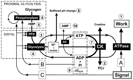
The system is as follows: proximal glycolysis (glycogen to HMP) includes glycogen phosphorylase (two forms, a and b); distal glycolysis (HMP to lactate) includes phosphofructokinase (PFK). ATP and ADP + P_i are exchanged between glycolysis and the myosin ATPase; ATP is buffered by creatine kinase (CK) at the expense of PCr, the net process consuming protons. Letters refer to regulatory influences (see Discussion). The signal which activates contraction (A) may stimulate glycolysis either by a closed-loop feedback mechanism (B) (e.g. via ADP, P_i, AMP or ΔG_ATP, which increase as ATP supply-demand mismatch lowers PCr), or by open-loop parallel activation (C). Numbers refer to calculations employed in this paper (see Methods). From the work rate (1) and the rate of PCr splitting (2), we infer glycolytic ATP synthesis (3); from this we obtain the distal glycolytic rate (4), and using changes in HMP (5) we obtain from this the proximal glycolytic rate (6). The distal glycolytic rate (3) gives lactate production, and by subtracting the proton consumption by PCr splitting (7), we calculate the net proton load (8) available to acidify the cytosol, and thus the buffer capacity. The diagram also shows (9) the contributions of ADP, ATP and P_i to the free energy of ATP hydrolysis (ΔG_ATP), and (10) the equilibrium between AMP, ADP and ATP catalysed by adenylate kinase (AK). ADP concentration is calculated from the creatine kinase equilibrium, AMP from the adenylate kinase equilibrium.

Measuring ATP production via creatine kinase

In terms of ‘energy balance’, ATP hydrolysis by the myosin ATPase is used to do mechanical work, ATP → ADP + P_i, while creatine kinase allows near-simultaneous rephosphorylation of ADP at the expense of PCr:

The sum of these two processes is the apparent net hydrolysis (‘splitting’) of PCr, the Lohmann reaction (Kushmerick, 1997):

which supplies 1 ‘ATP unit’ of energy per PCr. Thus creatine kinase ‘buffers’ ATP against temporal change, maintaining a near-constant concentration, while the much lower concentration of ADP undergoes proportionally large changes (Connett, 1988; Kemp, 1994). (This temporal buffering action is in addition to the ‘spatial buffering’ action of creatine kinase, which minimises spatial concentration gradients; Meyer et al. 1984.)

This system ensures, as a simple matter of chemical equilibrium, that PCr splitting automatically accompanies any mismatch between ATP use and ‘metabolic’ ATP supply (Kemp, 1994); furthermore the rate of PCr depletion (D = -d[PCr]/dt) is a quantitative measure of this mismatch (no. 2 in Fig. 1). In ischaemic exercise the sole ‘metabolic’ source of ATP is glycogenolysis to lactate, while in ‘pure’ aerobic exercise oxidative metabolism to CO₂ makes by far the largest contribution, and of course all intermediate cases exist. In any case, at the start of exercise, the initial PCr depletion rate is an estimate of the ATP turnover rate (F) (Foley & Meyer, 1993) (see eqns (22)-(31) below for how initial D is estimated). This is used to calculate ATP turnover throughout exercise (Conley et al. 1997; Kemp, 1997) (no. 1 in Fig. 1), by taking account of work rate (power). At any time:

(4)

based on the reasonable assumption that contractile efficiency is constant with time (see Discussion).

Measuring the rate of glycolysis

In general, glycolytic rate in ischaemic exercise can be estimated using ³¹P MRS in two ways. First, we can assume we understand proton handling and use this to estimate lactate accumulation, and thus glycolytic ATP synthesis (Kemp et al. 1994; Conley et al. 1997). However, we wish to study proton handling rather than assume it, and so we use a second approach: we assume we understand the relationship between work rate and ATP turnover, and use this to estimate glycolytic ATP synthesis and thus lactate accumulation (Wackerhage et al. 1996; Conley et al. 1997). We proceed as follows.

We saw above how to use initial PCr depletion rate and measured work rate to estimate total ATP turnover rate at each point (eqn (4)). This is the sum of the rates of ATP generation by glycolysis (L) and by PCr splitting (D), so by measuring D at each point, we can estimate glycolytic ATP synthesis rate (no. 3 in Fig. 1) as:

(5)

Glycolytic ATP production is related to lactate synthesis, with a stoichiometry of 3 ATP/glucosyl unit = 3/2 ATP/lactate. This factor is based on theory (Sahlin, 1978; Hultman & Spriet, 1986) and experimental data (Vezzoli et al. 1997; Hsu & Dawson, 2000). (An alternative factor (Conley et al. 1997) has been criticised (Hsu & Dawson, 2000) and corrected (Conley et al. 1998, 1999).) Thus the carbon flux through the ‘distal’ part of the glycolytic pathway (phosphofructokinase and beyond) is estimated (no. 4 in Fig. 1) as:

(6)

‘Proximal’ glycolytic flux (through phosphorylase) may temporarily exceed ‘distal’ flux, resulting in an accumulation of hexose monophosphates (HMPs), of which the main constituents are glucose 6-phosphate (≈80 %), fructose 6-phosphate (≈15 %) and glucose 1-phosphate (Hultman & Spriet, 1986; Chasiotis et al. 1987; Spriet et al. 1987a,b). Usefully, HMPs comprise most of the PME peak in the ³¹P MRS spectrum (the contribution of inosine monophosphate being negligible unless there is appreciable loss of ATP, which in the present work there is not). Thus the carbon flux through proximal glycolysis is estimated (nos 5 and 6 in Fig. 1) as:

(7)

and the glycogenolysis/glycolysis ratio is:

which approaches 1 as HMP concentrations become stable.

Analysis of ‘proton balance’

We now analyse the interactions between ATP turnover and intracellular acid-base physiology. Our aim is to use measured changes in PCr and pH, and inferred changes in lactate, to estimate the net proton load added to the cytosol during exercise, then by comparing this with the resulting pH change, to estimate intracellular buffering capacity. We will consider first the creatine kinase system on its own, and coupled to ATP hydrolysis; next we consider glycolysis on its own, then coupled to ATP hydrolysis; lastly we put all these together to calculate the net proton load.

The proton stoichiometry of creatine kinase

We have considered creatine kinase in technical terms in the estimation of free ADP (eqn (1)), and in physiological terms as an ATP buffer with applications in the measurement of ATP turnover (eqns (4) and (5)). To analyse its role in proton handling we must introduce explicit proton stoichiometry into the earlier equations:

where γ =α+ρ (we use the notation of Kushmerick (1997), but substituting ρ for β to avoid confusion). Thus ‘proton balance’ calculations are essentially about balancing charges; the coefficient γ balances charges in the Lohmann reaction:

To a first approximation PCr has charge -2 and P_i has charge φ - 2, so -γ≈φ≈ 0.4 at pH 7, as used in Harkema & Meyer (1997) and Wolfe et al. (1988); protons are consumed, increasingly as the pH is reduced. More detailed analysis (Kushmerick, 1997), taking account of K⁺ binding to PCr and P_i, suggests that this should be a smaller number (≈0.2 at pH 7), given empirically by:

(8)

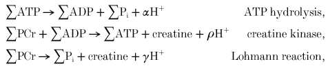
Details of this are given in the Appendix and Fig. 12.

Figure 12. Free fractions, stoichiometric factors and net charge.

A, the stoichiometric factors used in calculations as a function of pH. The filled symbols show the factor γ used here for the Lohmann reaction, and its components α for ATP hydrolysis and θ for creatine kinase. These are all empirical expressions from Kushmerick (1997): γ is given as eqn (8), and (for completeness) α= 39.108 - 19.262pH + 3.0662(pH)² - 0.15682(pH)³ and θ= -11.869 + 5.6685pH - 0.92213(pH)²+ 0.047950(pH)³. A also compares the coefficient of the Lohmann reaction (taken here as positive, i.e. protons consumed per PCr hydrolysed) in three published treatments; by ‘traditional’ factor is meant φ= 1/[1 + 10^{(pH - 6.8)}] used in Kemp & Radda (1994) based on Wolfe et al. (1988) and called θ in Walter et al. (1999), given in a similar form in Harkema & Meyer (1997), and as a similar value in Boska (1994); ‘revised’ factor means -γ (Kushmerick, 1997) which allows for K⁺ binding, as used here; ‘variant’ factor means φ - 0.15 as used in Newcomer & Boska (1997) and Newcomer et al. (1999). B, the free fractions of the metabolites used in calculations (eqns (A1), (A6) (A7) and (A8)), plotted as a function of pH: these are ADP (eqn (A3)), PCr (eqn (A4)), AMP (eqn (A5)), P_i (eqn (A9)), with ATP (eqn (A2)) on a different scale. (Note that this is not the same as Fig. 6C in (Kushmerick, 1997), which shows the fractions not bound to Mg²⁺ or K⁺.) C, the ratios of free fractions used in the pH correction of equilibrium constants and ΔG_ATP: these are for creatine kinase, the ratio f_ADPf_PCr/f_ATP (eqn (A1)), for adenylate kinase (f_ADP)²f_AMP/f_ATP (eqn (A6)), for ATP hydrolysis f_ATP/(f_ADPf_Pi) (eqn (A7)), and for the Lohmann reaction f_PCr/f_Pi (eqn (A9)). D, the net charge on PCr and P_i as a function of pH, using f_Pi and f_PCr (from B: eqns (A4) and (A9)): the difference between these two is the stoichiometric factor γ (see A).

The proton stoichiometry of glycolysis

Glycolytic ATP production in ischaemic exercise is almost entirely from glycogen (as muscle contains negligible free glucose, and the activity of glycogen phosphorylase far exceeds that of hexokinase). This can be written as:

where Φ depends on the charges of P_i, ATP and ADP: thus although lactate and H⁺ are produced, the net H⁺ production depends also on the ionisation states of ATP, P_i and ADP (Hochachka & Mommsen, 1983). However, this is not the whole story. If creatine kinase were absent, then simultaneous ATP hydrolysis would be required to maintain constant [ATP]. The result of these two processes would be:

where ATP synthesis and hydrolysis have cancelled out: so glycolysis in the absence of creatine kinase simply produces 1 H⁺ per lactate at steady state (Hochachka & Mommsen, 1983) (no. 4 in Fig. 1). (It also follows that Φ = (2/3) - α≈ -0.06 at pH 7, near zero; thus glycolysis + ATP hydrolysis alone is nearly proton neutral (Hochachka & Mommsen, 1983).)

The proton stoichiometry of glycolysis in the creatine kinase system

Having established the stoichiometry of the creatine kinase system and of glycolysis in isolation, we must now consider them in combination. The simplest approach is to say that, by conservation, the glycolytic proton production rate must equal the rate at which protons are buffered by passive processes (when pH changes) and consumed by net PCr breakdown (whether or not pH changes) (Mainwood & Renaud, 1985; Kemp & Radda, 1994). Thus pH change (no. 8 in Fig. 1) results from the difference between the rate of glycolytic proton production and proton consumption by net PCr breakdown (nos 4 and 7 in Fig. 1): as the former eventually dominates, pH will fall.

As a number of different approaches have been advocated (e.g. Hochachka & Mommsen, 1983; Kemp & Radda, 1994; Boska, 1994; Arthur et al. 1997; Kushmerick, 1997; Newcomer & Boska, 1997; Conley et al. 1998, 1999; Walter et al. 1999) (see also Appendix), we give an explicit argument for our approach. Suppose a fraction Ω of ATP demand is supplied by glycolysis: then the following processes are occurring. First, ATP hydrolysis (at unit rate), as above:

Also glycolytic ATP synthesis at rate Ω:

ATP hydrolysis outpaces glycolytic ATP synthesis by 1 - Ω, so creatine kinase makes up the difference:

Conceptually, ATP hydrolysis is divided into a fraction Ω which is opposed by glycolytic ATP synthesis, and a fraction 1 - Ω opposed by creatine kinase. The sum of ATP hydrolysis at rate Ω and glycolytic ATP synthesis at rate Ω is net glycolytic ATP synthesis at rate Ω:

The sum of ATP hydrolysis at rate 1 - Ω and creatine kinase at rate 1 - Ω is the Lohmann reaction at rate 1 - Ω:

In turn, the sum of these is:

Thus for each ATP used, the net proton load is the 2Ω/3 protons from lactate, less the (1 - Ω)(-γ) protons consumed by the Lohmann reaction. The total H⁺ load is the difference between lactate accumulation (proton generation) and net H⁺ consumption by PCr splitting: all other processes cancel out.

Estimating the net proton load

Now we can estimate the net proton load. First, lactate accumulation is estimated as:

(9)

where Δ indicates a change from basal. This is the amount of protons added to the cytosol by glycolysis. The total H⁺ load is then the difference between this and net H⁺ consumption:

(10)

Note that when pH changes as well as PCr, ∫γd[PCr]=/γΔ[PCr], so the amount of protons consumed by a change in pH and PCr depends on the route by which it is achieved. In practice the integrals are evaluated over n spectra as a spectrum-on-spectrum sum; thus ∫γd[PCr] is really Σ₁ⁿ(γδ[PCr]), where δ represents the change between successive spectra.

Because of the way L is calculated (eqn (5)), estimated lactate change in a single measurement interval is:

(11)

bearing in mind that δ[PCr] is negative, and so:

(12)

bearing in mind that γ is negative.

Estimating buffer capacity

Given the net proton load, we can now estimate buffer capacity (β) according to the general equation:

(13)

which we use in three ways, as follows.

Buffer capacity at the start of exercise

At the start of exercise (i.e. the first spectral collection interval), assuming negligible lactate production, β is estimated as a simple ratio:

(14)

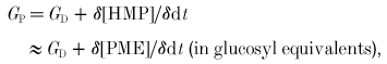
To obtain the true cytosolic buffer capacity (β_C) we must subtract from this the contributions of P_i and PME (β_P =β_Pi+β_PME). These are calculated as follows. For a simple buffer acid ⇋ base⁻+ H⁺, the Henderson-Hasselbalch equation (the logarithmic form of the equilibrium expression) states:

where C is the total concentration and a the concentration of the acid form, and pK = -logK, where K =[base⁻][H⁺]/[acid] is the acid dissociation constant (Roos & Boron, 1981). The theoretical buffer capacity can be found by differentiation as:

(15)

with pK_x = 6.8 for P_i and 6.2 for PME (Conley et al. 1997). More conveniently, β_Pi = 2.3[P_i]φ(1 - φ). Notice the distinction between the contribution of P_i generated in a time increment to the charge balance that results in net consumption of H⁺ during PCr splitting (see above, eqn (8)), and the contribution of pre-existing P_i to the passive buffering of the (negative) proton load that results from this (eqn (13)).

Overall buffer capacity throughout exercise

An estimate of overall, all-exercise average buffer capacity (including the increasing contribution of P_i and PME, and any effects of pH change on β_C) could be obtained by linear regression, using:

(16)

then subtracting the average all-exercise contributions of P_i and PME (eqn (15)). We use a modified approach in which the contribution of P_i and PME is subtracted before the linear regression: we correct the cumulative proton load (the numerator in eqn (16)) by subtracting the cumulative protons buffered by P_i and PME, which is -∫β_PdpH, or in practice -Σ₁ⁿ(β_PδpH). Thus:

(17)

Note that, in general, ∫βdpH =/β∫dpH, so the amount of protons buffered by a change in pH depends on the route by which it is achieved.

True buffer capacity throughout exercise

The previous approach ignores the pH dependence of true buffer capacity, β_C. A better approach uses a least-squares fit of proton load to pH over the whole of exercise, solving for resting β_C and the pH dependence of β_C. There are several possible methods, but here we assume a ‘physicochemical’ dependence of β_C on pH (analogous to eqn (15)), as if a single buffer species were involved:

(18)

The aim is to match the non-P_i proton load (numerator in eqn (17)) and the amount buffered by non-P_i cytosolic buffers, which is:

(19)

Using this to define the pK and concentration of buffer species (Wolfe et al. 1988) would involve unacceptable extrapolation; rather we express β_C relative to its resting value, and solve for resting β_C and notional pK. (We constrain β_C to lie between the extreme values given by eqn (14) across all the subjects.) It will be seen later that the relationship between β_C and pH is close to being linear.

Apparent buffer capacity

Lastly, a functional ‘apparent’ buffer capacity can be defined as -δ[lactate]/δpH, and includes a contribution due to PCr splitting. This has no simple physicochemical meaning, but is useful for comparison with biopsy data (Sahlin, 1978) (see Discussion).

Analysis of metabolic control

Principles

In aerobic exercise, in the long term, ATP production must be matched to ATP use (i.e. to work rate). The mismatch between ATP use and production is (to a first approximation) the rate of fall of PCr, so that change in PCr can be thought of in engineering terms as the error signal in an integral control feedback loop (Kemp, 1994, 2000). This fits neatly with the idea that the mitochondrion is controlled by [ADP], which rises as [PCr] falls (Chance et al. 1985). Whether this does occur is outside the scope of this paper, but we make use of the idea of a mismatch signal. In ischaemic exercise the muscle is a closed system, and therefore exercise is not sustainable; indeed if PCr did come to steady state a valuable sink for glycolytic protons would disappear. Nevertheless, within the pH constraints, we can assume that matching glycolytic ATP production to ATP use is an important function of the system. We can describe the properties of the system, in a purely formal way, by plotting glycolytic flux against the mismatch signal -Δ[PCr].

Control of glycogen phosphorylase

In aerobic exercise, it has often been argued that some function of the primary mismatch signal (whether ADP or ΔG_ATP) is causally significant, by having a dominant effect on mitochondrial ATP synthesis) (Kemp, 2000). It has long been suggested that P_i, which also increases as PCr falls, may play a similar role in control of glycogenolysis (Griffiths, 1981). Attention has focused on glycogen phosphorylase and phosphofructokinase. Increased flux to lactic acid requires increased flux through glycogen phosphorylase (as through all pathway enzymes), and this requires either an increase in substrate, or some allosteric mechanism. Little is known about how phosphorylase rate is influenced by glycogen concentration. It is assumed that increases in phosphorylase flux are achieved by two means: first, the conversion of ‘inactive’ phosphorylase b to ‘active’ phosphorylase a, mediated by the Ca²⁺-activated enzyme phosphorylase b kinase, and second by the increase in the concentration of the co-substrate P_i as a consequence of the PCr splitting (Chasiotis, 1983; Yamada et al. 1993). If this is true, then assuming Michaelis-Menten kinetics as seen in vitro (Chasiotis, 1983):

(20)

where G_MAX is the maximum activity of phosphorylase a under prevailing conditions and K_Pi (= 26 mm) is the [P_i] at which the activity of phosphorylase a is half maximal in vitro (Chasiotis, 1983). This simply states the consequence of phosphorylase behaving the same in vivo and in vitro. Making this provisional assumption, we estimate the ‘maximum activity’ (i.e. notional activity at saturating [P_i]) of phosphorylase a at each point as:

(21)

expressed here in three-carbon (lactate equivalent) units rather than ATP units as before (Kemp et al. 1996; Kemp, 1997). This assumes the truth of the eqn (20), and asks what the implications are for the activation state of phosphorylase. Its main use is to distinguish stimulation of glycogenolysis resulting from increase in the enzyme (i.e. b-to-a conversion) from that arising from increase in [P_i].

Control of distal glycolysis

We can also distinguish glycogenolysis from glycolysis (they are different in early exercise). In a simplistic view of a two-stage process we can consider glucose 6-phosphate as the substrate of distal glycolysis (beginning with phosphofructokinase), and HMP as a measure of this: thus we can relate the distal flux to its substrate.

Estimating initial PCr depletion rates during exercise

Estimates of lactate production and therefore buffer capacity during exercise depend heavily on initial ATP turnover rate, measured as the initial rate of PCr depletion (D). This is calculated in several different ways (we discuss later which is best: see Fig. 3).

Figure 3. Phosphocreatine depletion rates during ischaemic exercise.

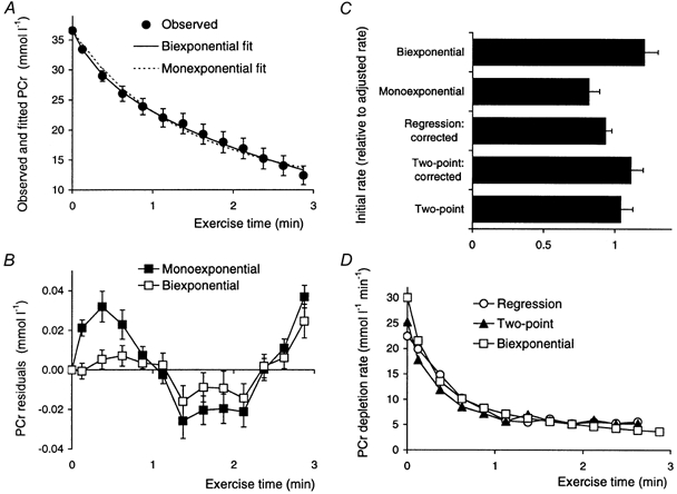
A, the observed time course of phosphocreatine (•) together with lines showing the results of fitting to monoexponential and biexponential kinetics. The monoexponential fit is eqn (24) with Δ[PCr]= 30 ± 4 mmol l⁻¹, and k = 0.7± 0.1 min⁻¹ (corresponding to t_1/2 = 1.4 ± 0.5 min). The biexponential fit is eqn (27) with Δ[PCr]_A = 6 ± 1 mmol l⁻¹, Δ[PCr]_B = 30 ± 2 mmol l⁻¹, k_A = 3.7 ± 0.8 min⁻¹ (corresponding to t_1/2 = 0.5 ± 0.3 min) and k_B = 0.31 ± 0.04 min⁻¹ (corresponding to t_1/2 = 0.31 ± 0.04 min). B, the residuals (observed minus fitted) for these two fits, scaled to resting phosphocreatine concentration. C, the estimated initial rates of phosphocreatine depletion (expressed as a fraction of the adjusted value described in the text and in Fig. 6), measured in five different ways: from monoexponential (eqn (25)) and biexponential fits (eqn (28)), from the difference between the basal and first-exercise point as measured (eqn (22)), and ‘corrected’ to t = 0 using the monoexponential rate constant (eqn (23)), and by three-point linear regression, extrapolated to t = 0 (eqn (30)). D, the time course of phosphocreatine depletion rate calculated in three of these five ways: regression, two-point corrected and biexponential fit (eqns (23), (29) and (30)) (the monoexponential fit (eqn (26)) is obviously inappropriate). Error bars show s.e.m. (omitted in D).

Estimates from consecutive spectra

The simplest rate estimate is obtained from spectrum-spectrum differences:

(22)

Because of the curvilinear time course of PCr, this might be expected to underestimate the true rate (-d[PCr]/dt), especially in the early phase. An approximate correction is available using the monoexponential PCr rate constant k (see below), which in effect corrects each rate to the start of the measurement interval (Kemp et al. 1994):

(23)

This is theoretically correct for pure monoexponential kinetics (although not in that case the best way to estimate D: see next paragraph). However, it might be a partial correction even though the monoexponential fit to PCr is, as we shall see, not good. (However, as we will show, the uncorrected rate may, paradoxically, be more correct.)

Estimates from exponential fits

By analogy with the typical analysis of aerobic exercise (Meyer, 1988), we can attempt to fit [PCr] to a monoexponential function:

(24)

where -Δ[PCr]_SS is the implied steady state value and k is the rate constant, which is inversely proportional to the half time (k = 0.693/t_1/2). In the present work we constrain -Δ[PCr]_SS to be less than basal [PCr], so that implied steady state [PCr] is positive, although not doing so makes very little difference to the fit or the calculated initial D. The derivative of eqn (24) can be used to calculate initial rate directly as:

(25)

and rates throughout exercise as:

(26)

This analysis of PCr kinetics in ischaemic exercise lacks the theoretical underpinning of its application to aerobic exercise (Mahler, 1985; Meyer, 1988; Kemp, 1994), and no true steady state is possible. Also, we will show later (see Results) that the fit is not good.

A more general approach is to use a biexponential fit to PCr, which can be written:

(27)

where the subscripts refer to the two separable components. Analogous to the monoexponential case, rate of PCr depletion can be obtained as:

(28)

(29)

Notice that this still implies a steady state at which -Δ[PCr]_SS = -Δ[PCr]_A+ -Δ[PCr]_B. The fitted parameters in eqn (27) are much more sensitive to constraints than in the monoexponential case, although the quality of the fit and the initial rate are not. Again we constrain the fit so that the implied steady state [PCr] is positive.

Regression estimates

Although linear regression estimates (here, the regression slope of [PCr]vs. time for three consecutive spectra) obviously underestimate true rates, it will be seen that the error in later exercise is small. To benefit from the smoothing effect, we use this method from the third exercise point onwards. Three-point regression slope estimates are assigned to the time point of the middle spectrum. To approach the true initial rate more closely, we obtain two successive regression estimates of PCr rate (call these D′₁, measured from rest to exercise spectrum 2, assigned to t₁, the time of the first spectrum, and D′₂, measured from exercise spectrum 1 to spectrum 3, and assigned to t₂). We then extrapolate back to t = 0 to obtain:

(30)

Estimates adjusted by a buffering analysis

In experiments with sufficient time resolution, it is possible to distinguish an early cellular alkalinisation before the later progressive acidification (see Fig. 2). This provides a method of correcting any estimate of initial ATP turnover, by requiring that the line joining successive points on a graph of net proton load against pH change passes through the origin between the initial point(s) where pH change is positive and the subsequent point where it becomes negative (in this work this is the first spectral interval in 2 subjects, the second in 5 and the third in 2 subjects). This works as follows: let P_a and ΔpH_a be the cumulative proton load and pH change from basal, respectively, at the last spectral-collection point for which ΔpH is positive (i.e. just before the pH falls below basal), while P_{a+ 1} and ΔpH_{a+ 1} are the values at the next spectrum. Then the proton load at the point where the cumulative pH change is zero (i.e. where the pH passes the basal value on its way down) is given by:

(31)

Now:

where δt_a is the time interval between spectrum a and its predecessor over which the concentration changes δ[PCr]_a and δ[lactate]_a are measured, F is the total ATP turnover rate appropriate for that interval, and γ is the appropriate value of the stoichiometric factor (we simplify the expression by assuming F and γ to be constant near the start of exercise). Similarly:

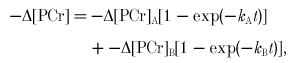
Figure 2. Time course of pH and metabolite concentrations during ischaemic exercise.

A, cytosolic pH. B, the concentrations of phosphocreatine, and of inorganic phosphate and its two ionic components. C, phosphomonoester concentration. D, the concentrations of free ADP and free AMP (note logarithmic scale). E, the free energy of ATP hydrolysis. Error bars show s.e.m.

Substituting for P_{a+ 1} and P_a in eqn (31), we can find the value of F which makes P_{ΔpH = 0} = 0, by numerical solution, starting from the corrected linear regression estimate (eqn (30)).

Calculation of constraints and simulation of exercise

Constraints

To illustrate the constraints under which muscle metabolism exists, we calculate some extreme combinations of measurements (methods largely as in Kemp (1997), but using the new stoichiometric constant -γ (Kushmerick, 1997) and full numerical solutions). First, some absolute constraints.

Zero lactate production is modelled by numerical solution of:

(32)

Zero pH change is modelled by numerical solution of:

(33)

Zero PCr change is modelled by numerical solution of:

(34)

In each case the result is made time dependent using:

(35)

Next we calculate lines (isopleths) that connect points with same concentration.

Lines of constant lactate are given by:

(36)

Lines of constant [ADP] can be directly calculated from the simple version of the equation for [ADP] (eqn (1) above). Thus for a given [ADP]:

(37)

which gives the required [PCr] for a given pH. The translation of pairs of pH and [PCr] into ‘consumed protons’∫γd[PCr] and ‘buffered protons’ -∫βdpH is not unambiguous, as γ depends on pH, and β depends on P_i and pH (the earlier treatment of this was oversimplified in this respect; Kemp, 1997). A convenient method is to imagine reaching the required pH and PCr in two stages, each made up of very small increments: first changing PCr at constant pH, so that consumed protons =γ∫d[PCr]; then changing pH at constant [ADP], so that buffered protons = -∫βdpH (remembering that β is a function of pH, even though PCr, and therefore P_i, is being held notionally constant). The corresponding [lactate] is then the sum of the buffered and consumed protons.

Simulations

We will also examine some consequences of hypothetical variations in the kinetics of glycolytic rate. This can be performed in a time-independent or time-dependent manner (Kemp, 1997); here we use the latter, calculating for each small time increment:

(38)

(39)

(40)

A note on units

As concentrations are calculated per litre cytosolic water, the convenient unit of flux is millimoles per litre per minute. It will be seen that much of the interpersonal variability in e.g. rates of glycolysis is explained by variation in total ATP turnover rate. For this reason it will sometimes be useful to express the glycolytic ATP synthesis rate or the rate of PCr splitting as a fraction of the initial ATP turnover rate (e.g. Figs 7-9); these ‘relative’ ATP synthesis rates are dimensionless ratios, with maximum value 1. The relative rates of carbon fluxes (i.e. 6-carbon or 3-carbon fluxes) can also be expressed relative to the initial ATP turnover rate (e.g. Fig. 7B): the results are dimensionless ratios with no necessary upper limit. We will also sometimes ‘scale’ the changes in metabolites by dividing by the initial ATP turnover rate (Fig. 8); scaled change in [PCr] and scaled cumulative glycolytic ATP synthesis have units of minutes, and scaled change in ΔG_ATP has units MJ l min mol⁻².

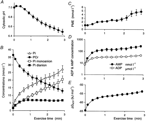
Figure 7. Metabolic fluxes during ischaemic exercise.

A, ATP synthesis rates: the total rate (eqn (4)), the rate of PCr splitting (adjusted rates, as in Fig. 6A), and the rate via glycolysis (eqn (5)). B, the rates, relative to initial ATP turnover rate, of ATP synthesis by PCr splitting and by glycolysis. C, rates of lactate production (= distal glycolysis, expressed as lactate, i.e. 3-carbon, flux; eqn (5)) and of glycogenolysis (= proximal glycolysis, expressed as glucosyl, i.e. 6-carbon, flux; eqn (7)). D, the ratio of glycogenolysis to glycolysis (i.e. proximal to distal glycolysis, each expressed in the same units). Data are means ±s.e.m.

Figure 9. Metabolic fluxes and some metabolite concentrations during ischaemic exercise.

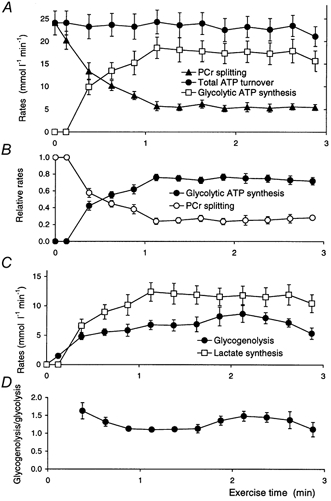
A, the glycolytic ATP synthesis rate as a function of P_i concentration. B, the rate of glycogenolysis (in 3-carbon units), and its notional maximum rate (G_MAX) at excess P_i concentration (eqn (21)) throughout exercise. C, the rate of distal glycolysis (in 3-carbon units) as function of phosphomonoester concentration. All fluxes are expressed relative to initial ATP turnover rate. Data are means ±s.e.m.

Figure 8. Metabolic fluxes and some metabolite concentrations during ischaemic exercise.

The figure shows the glycolytic ATP synthesis rate plotted as a function of several quantities: the change in PCr concentration (A), the change in free energy of ATP hydrolysis (B), and the cumulative amount of glycolytic ATP synthesis (C). In each case both the glycolytic ATP synthesis rate and the quantities on the x-axis have, to minimise intersubject variability, been divided by the initial ATP turnover rate. Data are means ±s.e.m.

RESULTS

Metabolites and pH (Fig. 2)

Resting values (±s.e.m., n = 9) before the onset of exercise were:

Figure 2 shows pH and metabolite concentrations as a function of time during ischaemic exercise. As usual in such studies, pH decreases after a transient increase (Fig. 2A); PCr concentration decreases monotonically, and P_i concentration increases approximately stoichiometrically (Fig. 2B): it can be seen that the increase in P_i concentration was predominantly in the monoanionic form (which is thought to be the form most important in the development of fatigue; Miller et al. 1988; Cady et al. 1989), as the concomitant fall in pH almost exactly balances the generation of P_i, so that P_i dianion concentration reaches a plateau value early on (Fig. 2B). PME concentration increased also in an approximately biphasic manner (Fig. 2C). Calculated free ADP and AMP (Fig. 2D), and ΔG_ATP (Fig. 2E) all increased in an approximately biphasic way.

PCr depletion rates (Fig. 3)

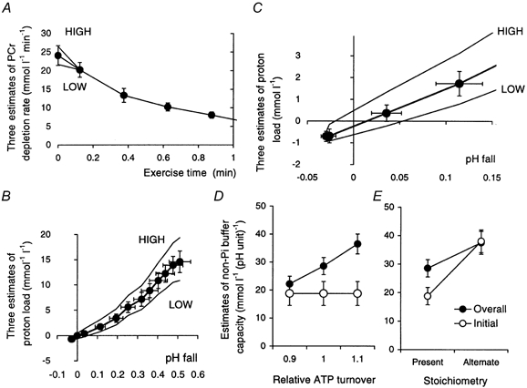
To calculate relevant metabolic fluxes, we must first estimate the initial rate of PCr depletion. As explained in Methods, there are a number of possible ways to do this. Figure 3A shows the observed PCr concentrations and the monoexponential and biexponential fits; both are less than adequate, as can be seen from the non-random residuals (Fig. 3B), the monoexponential fit being significantly worse towards the start of exercise. Comparing the different estimates of initial rates (Fig. 3C), that from the monoexponential fit is lowest, consistent with the larger residuals; the biexponential value is the largest, followed by the two-point value corrected using the monoexponential rate constant, then by the uncorrected two-point value; the value from linear regression is lower than these two, despite the linear extrapolation to t = 0 (Fig. 3C). The time course of some of these rate estimates is shown in Fig. 3D; the differences are only crucial at the start of exercise. The initial rate estimates in Fig. 3C are shown as a fraction of the adjusted value of D = 25± 3 mmol l⁻¹ min⁻¹, whose derivation takes account of proton buffering in the first few intervals (see Methods): this will be presented later, after the rest of the proton buffering results.

Proton handling (Figs 4 and 5)

Figure 4. Proton handling during ischaemic exercise.

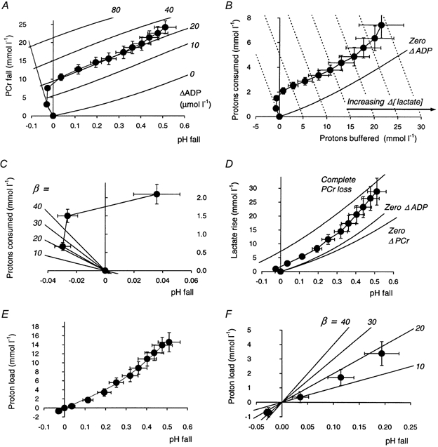
The figure shows several quantities plotted in a time-independent, cumulative manner during exercise. A, the fall in PCr as a function of that in pH; the lines in the background represent lines of constant suprabasal ADP concentration, varying from no increase in ADP to ‘infinite’ ADP, i.e. complete PCr depletion (calculated from eqn (37)). B, the cumulative amount of protons that this process ‘consumes’ (∫γd[PCr]), plotted as a function of the cumulative amount of protons ‘buffered’ (-∫βdpH); the continuous line represents no increase in ADP (calculated from eqn (37)); lines of constant non-zero increase in ADP could be plotted above this, as in Kemp (1997), but are omitted here for clarity. The dashed lines show constant lactate change (eqn (36)); for each, Δ[lactate] is simply equal to the x-co-ordinate. C, an expansion of the initial region of a plot of protons ‘consumed’ (∫γd[PCr]) as a function of pH fall: the lines radiating from the origin represent nominal values of buffer capacity as indicated (calculated from eqn (13)); the initial (alkaline) point corresponds to a buffer capacity of 20 mmol l⁻¹ (pH unit)⁻¹ (see Results), before lactate production moves the data points in the direction of acidification despite progressive proton consumption by continuing PCr hydrolysis. D, the amount of lactate accumulated as a function of pH fall; the slope of this line is the apparent buffer capacity -d[lactate]/dpH. E, the net proton load to the cytosolic buffers (i.e. the difference between lactate production and proton consumption by PCr splitting (eqns (10) and (12)) as a function of pH fall: the slope of this line (-d[H⁺load]/dpH) is an estimate of true buffer capacity. F, an expanded view of the near-rest region in E, with lines of constant buffer capacity (from eqn (13)). Error bars show s.e.m.

Figure 5. Proton handling during ischaemic exercise.

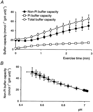
A, the total buffer capacity (from eqns (18) and (19)), the buffer capacity due to P_i and PME (eqn (15)), and their difference, the true cytosolic buffer capacity during exercise. B, the true cytosolic buffer capacity as a function of pH. Error bars show s.e.m.

We now consider the intracellular handling of protons. Figure 4A shows the relationships between the cumulative changes in pH and PCr concentration. This plot also shows lines of constant ADP concentration (which is a function of pH and PCr), and the line at the left-hand edge represents a notional line of zero lactate production. Figure 4B, derived from Fig. 4A, shows the amount of H⁺‘consumed’ by PCr splitting plotted as a function of the amount of protons remaining to be ‘buffered’ passively: the sum of these two quantities is equal to the change in lactate concentration, and Fig. 4B also shows (dotted) lines of constant lactate accumulation, which are cut successively by the data points as exercise proceeds. Figure 4B also shows the line of zero increase in ADP, derived from that shown in Fig. 4A. One could also calculate more lines of constant ADP increase, as in Fig. 4A; a simplified version of such a plot has been presented elsewhere (Kemp, 1997), although, strictly, the amount of protons consumed by PCr hydrolysis between the origin and a point of given pH and PCr depends somewhat on the route taken, as the amount of proton consumption is pH dependent (see Methods).

Figure 4C shows an expanded view of a plot of protons consumed by PCr hydrolysis against pH change in the early stages of exercise. Initial H⁺ consumption, outweighing lactate production, causes an initial alkalinisation; if we assume that lactate production is negligible in this first interval, the first-exercise point corresponds to a non-P_i buffer capacity of 20 ± 3 mmol l⁻¹ (pH unit)⁻¹ (eqn (14)). Compare the first data point in Fig. 4C to the diagonally radiating lines of constant buffer capacity assuming no lactate production. In the absence of lactate production later in exercise the experimental point would (roughly) move further along the same line; instead, of course, lactate production causes acidification as PCr depletion continues.

Figure 4D shows the relationship between calculated lactate concentration and pH change. As in needle biopsy studies (Sahlin, 1978), other MRS studies (Wackerhage et al. 1996) and studies combining the two methods (Sullivan et al. 1994) this is near linear. From its slope we can calculate an apparent buffering capacity of 52 ± 6 mmol l⁻¹ (pH unit)⁻¹, comprising both true buffering (both by non-P_i cytosolic buffers and by P_i, whose concentration increases throughout exercise) and the H⁺-consuming effect of PCr splitting (see Methods). Of the total lactate (proton) load, we can calculate that 27 ± 2 % is consumed by the Lohmann reaction. Removing this component, we obtain an estimate of the net H⁺ load to the cytosolic buffers. Of this, 30 ± 5 % is buffered by pre-existing P_i and PME. Removing this component as well gives us the relationship between net H⁺ load to the cytosolic buffers and the pH change shown in Figs 4E and F: Fig. 4F concentrates on the first few time points, showing the data with lines of constant buffer capacity analogous to those in Fig. 4C, while Fig. 4E shows the full course. This relationship was approximately linear, with overall slope (a measure of overall non-P_i buffer capacity) of 28 ± 5 mmol l⁻¹ (pH unit)⁻¹. This overall slope is not very useful, in view of the likely pH dependence of cytosolic buffer capacity (see Discussion). There are several ways in which this pH dependence could be established, but here we have fitted the proton load-pH change data (Fig. 4E) assuming, notionally, a single buffer species whose effective pK turns out to be 5.5 ± 0.2 (the fit constrains pK to be between 5 and 7 - physiologically plausible, mathematically somewhat arbitrary, but making little difference to the fit). This fit (the line in Fig. 4E) yields the buffer capacity shown in Fig. 5A as a function of exercise time, and in Fig. 5B as a function of pH. Figure 5A also shows the buffer capacity due to P_i and PME, and the total buffer capacity. The true cytosolic (non-P_i, non-PME) buffer capacity increases from 20 ± 3 mmol l⁻¹ (pH unit)⁻¹ at rest to 48 ± 5 mmol l⁻¹ (pH unit)⁻¹ at the end of exercise. This is quite close to a linear pH dependence, with mean slope -dβ/dpH = 55 ± 7 mmol l⁻¹ (pH unit)⁻².

As PCr depletion rate decreases, and smaller amounts of protons are consumed by PCr splitting in each interval, the apparent buffer capacity (the slope of lactate against pH fall - see Fig. 4D) becomes closer to the true buffer capacity (the slope of net proton load against pH fall - see Fig. 4F).

Buffering and ATP turnover at the start of exercise (Fig. 6)

Figure 6. Phosphocreatine depletion rates and proton load estimates during ischaemic exercise.

A, the adjusted estimate of the rate of PCr depletion (initial rate from eqn (30) adjusted using eqn (31), then linear regression thereafter) during the first minute of exercise (•), together with two variations of the initial rate, 10 % higher and lower than the adjusted value. B, the relationship between proton load and pH calculated using the adjusted value of initial PCr depletion rate (•), and using the two variant values. C, an expanded view around the origin of the same data as B. D, the result of the variant error assumptions on the all-exercise average (eqn (16)) and initial-exercise (eqn (14)) estimates of buffer capacity. E, the result of an alternate assumption (see Methods) about the proton stoichiometry of PCr splitting on all-exercise average (eqn (16)) and initial-exercise (eqn (14)) estimates of buffer capacity. Error bars show s.e.m.

We return now to the initial rate of ATP turnover, and how this was adjusted using an analysis of proton handling in early exercise. It can be seen that the proton load vs. pH plot in Fig. 4E passes through the origin as acidification succeeds the initial alkalinisation. The slope of this plot is an estimate of buffer capacity (eqn (13)) both in the initial alkalinisation (eqn (14)) and the later acidification (eqn (17)), and so the slope should be the same on either side of the origin, at least reasonably so, before P_i accumulation increases the overall buffer capacity (eqn (15)). The line should therefore pass through the origin: that is, pH should have returned to basal values when lactate accumulation exactly matches the amount of protons consumed by PCr splitting in the first spectral acquisition interval, this being defined by linear interpolation between the data points immediately adjacent on opposite sides of the origin - usually the first and second exercise data points. As explained in Methods (eqn (31)), the initial rate of ATP turnover has been slightly adjusted so that this is so (this is the adjusted value to which other estimates are referred in Fig. 3D).

We need to define the effect of potential errors in the initial rate of ATP turnover. Figure 6A shows, for the first minute of exercise, the adjusted values of PCr depletion rate, together with two arbitrary variations of the initial rate, 10 % high and 10 % low. Figure 6B shows the proton load vs. pH fall relationship (as in Fig. 4F) assuming these three values of initial PCr depletion rate. The higher this is, the higher the apparent lactate concentration and therefore the higher the net proton load at any point. Figure 6C, which focuses on the first few points of the proton load-pH relationship (as in Fig. 4E), shows how the variant rate assumptions result in failure of the line to pass back through the origin on its way from the initial alkalinisation to the later, sustained, acidification. Figure 6D shows the resulting effects on the all-exercise mean estimate of cytosolic buffer capacity, which increases with assumed initial ATP turnover, and the initial-exercise estimate, which is independent of ATP turnover. We return to this in the Discussion.

Figure 6E makes a different point, showing the effects on the overall and initial-exercise estimates of buffer capacity of assuming a different value for the stoichiometric coefficient -γ, namely the earlier factor φ (Kemp & Radda, 1994). Again, we return to this in the Discussion.

Fluxes (Fig. 7)

We are now equipped to estimate some metabolic fluxes and study their relationships. Figure 7 shows fluxes as a function of time during exercise. The total ATP turnover, by definition, tracks the work rate (as contraction efficiency is taken to be constant). Figure 7A shows that estimated total ATP turnover, and therefore measured work rate, did not fall significantly during exercise. Thus despite subjective fatigue, all subjects were able to maintain a constant work rate.

Figure 7A also shows that the rate of PCr splitting decreased to a plateau value, so the rate of glycolytic ATP synthesis increased to a plateau during the course of the exercise. This has some resemblance to aerobic exercise (Meyer, 1988), where, however, the rate of PCr depletion eventually falls to zero and a true steady state is reached; this is impossible in ischaemic exercise where the muscle is a closed system, and continued glycolysis means continued lactate-proton accumulation.

To show these relationships better, obscured as little as possible by interpersonal variation, Fig. 7B shows the rates of ATP generation by PCr splitting and by glycogenolysis as a fraction of total ATP turnover. Figure 7B makes clear that much of the variation in the glycolytic rate seen in Fig. 7A is a consequence of intersubject variation in the rate of total ATP synthesis. The fraction of ATP provided by glycolysis in each spectral interval increases from zero at the start to 0.72 ± 0.05 at the end of exercise. Comparison of the changes in PCr (Fig. 4A) and lactate (Fig. 4B) shows that the whole-exercise average fraction of ATP provided by glycolysis, given by 1/{1 - (2/3)(Δ[lactate]/Δ[PCr])}, is 0.62 ± 0.03.

Figure 7C compares the absolute rates of glycolytic ATP synthesis (as in Fig. 7A) with the estimated rate of lactate production. It can be seen that these have roughly the same time course; these differ of course by a stoichiometric factor of approximately 3/2, depending on the relationship between the rates of proximal and distal glycolysis (see eqn (7)). This relationship can be seen more clearly in Fig. 7D, which plots the ratio of proximal to distal glycolytic rates. Proximal glycolysis exceeds distal at the start of exercise: this corresponds to the increase in PME (Fig. 2C), and represents a temporary excess flux through phosphorylase over that through phosphofructokinase, as is well known from needle-biopsy studies (Hultman & Spriet, 1986; Chasiotis et al. 1987; Spriet et al. 1987b); the ratio gradually approaches unity (expressed in appropriate units) as PME stabilises.

Relationships between fluxes and concentrations (Figs 8 and 9)

Next we consider the relationship between fluxes and some potentially relevant concentrations.

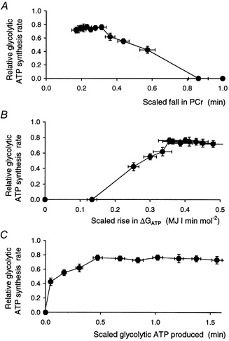
General ‘transfer functions’ (Fig. 8)

Given the data and the biochemical background (see Introduction and Methods), a natural ‘transfer function’ (if it can be so called) which characterises the system is the relationship between the rate of glycolytic ATP synthesis and the fall in PCr. This is shown in Fig. 8A, plotted relative to ATP turnover to reduce variability. It can be seen that after the initial lag, the relationship is near linear up to a break point, following which glycogenolysis remains at a plateau.

Because of the constraints imposed by the creatine kinase equilibrium (Connett, 1988; Kemp, 1994) this relationship implies other relationships, for example to [ADP] and [AMP] (not shown), and also to the free energy of ATP hydrolysis, ΔG_ATP. The last of these is plotted in Fig. 8B, which shows a quasi-sigmoid relationship somewhat resembling similar relationships for oxidative ATP synthesis in aerobic exercise (Jeneson et al. 1995, 1996).

Lastly, Fig. 8C shows the relationship between glycolytic ATP synthesis rate at a point and the total amount of glycolytic ATP synthesis up to that point. This shows that at least half the ATP is synthesised at a near-constant rate, albeit one that falls short of total ATP turnover, so that [PCr] continues to fall. This relationship is independent of the apparent lag in activation of glycolysis seen in Fig. 7A and B).

The relationships in Fig. 8 are rather abstract, related to the overall ATP economy and in particular the relationship between ATP synthesis and the need for ATP. We argue that they offer a way of characterising the system, particularly suited to the data that ³¹P MRS supplies, but they may contain no insight into mechanisms.

Possible causal relationships (Fig. 9)

We now consider some relationships that have some possible causal significance (to put it no more strongly). The relationship of glycolytic ATP synthesis against the rate of fall of [PCr] shown in Fig. 8A implies the relationship of glycogenolytic rate against P_i concentration shown in Fig. 9A. As noted elsewhere (Kemp et al. 1994; Kemp, 1997) this is roughly hyperbolic, at least reminiscent of the P_i dependence of phosphorylase a activity in vitro (Chasiotis, 1983; Ren & Hultman, 1990), except that it starts from a near-zero value at resting and near-resting [P_i]. Note that in the first exercise interval glycolytic ATP production and therefore lactate production are indistinguishable from zero, but the net accumulation of PME results in a small positive rate of proximal glycolysis.

Figure 9B, derived from Fig. 9A, shows the notional maximum rate of glycogenolysis, assuming a P_i dependence resembling that of phosphorylase a (see Methods). This is an attempt to estimate what glycolytic rate might be if P_i concentration were high enough that there was no question of it limiting the rate. As noted before (Kemp et al. 1994; Kemp, 1997), it increases from a near-zero value at rest and in the first interval, but is then at least approximately constant for most of the exercise. It can be seen from Fig. 9B that the period of its approximate constancy starts earlier than the plateau in glycolytic rate: thus from about 20-90 s the increase in glycogenolytic rate may be largely explained by the increase in P_i resulting from the fact that glycolytic ATP synthesis falls short of ATP demand.

Figure 9C shows a slightly different plot of the rate of distal glycolysis against PME, which can be considered the substrate for this block. The rate and the concentration increase together, the rate gradually flattening off to a plateau. This is discussed further below.

Relationships between metabolic regulation and proton handling (Figs 10 and 11)

Figure 10. Some absolute constraints on pH and metabolite changes during ischaemic exercise.

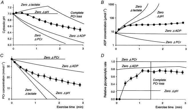
The figure shows some absolute constraints on pH and metabolite changes (A-C) by considering some extreme situations: no lactate production (eqn (32)) until all PCr is exhausted (eqn (34) with maximal [P_i]); lactate production in the absence of PCr depletion (eqn (34) with resting [P_i]); coordinated control of lactate production in relation to PCr depletion such that pH does not change (eqn (33)); and coordinated control of lactate production and PCr depletion such that ADP does not change (eqn (37)). D, the corresponding rates of glycolysis. All constraints are expressed in the time domain using eqn (35). These theoretical lines are as labelled. The observed data are shown as filled circles (means ±s.e.m.).

Figure 11. Effects of changes in the control properties of glycolysis on pH and metabolite changes during ischaemic exercise.

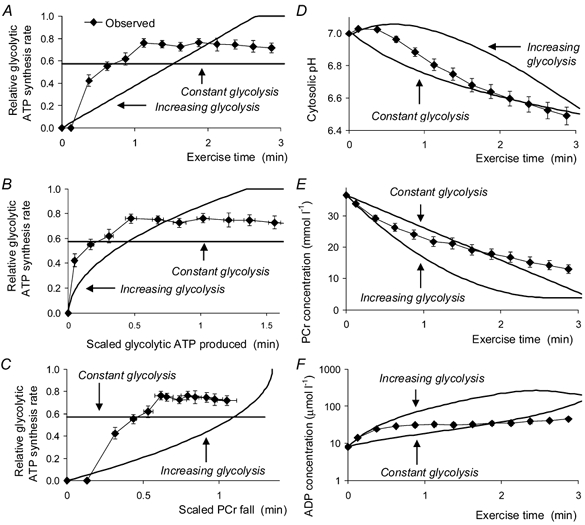
The figure shows the results of a simulation of two hypothetical cases: assuming glycolysis linear with time, and assuming glycolysis is constant. We assume that the total amount of lactate produced, the time taken and the rate of ATP turnover are the same as measured. Results are obtained by numerical solution of eqns (38)-(40). Left-hand panels show the glycolytic rate (as a fraction of total ATP turnover rate) plotted against exercise time (A), the total amount of glycolytic ATP synthesised (B) and the fall in PCr (C) (the latter two quantities scaled to ATP turnover). Right-hand panels show the changes in pH (D), PCr concentration (E) and ADP concentration (F). The theoretical lines are as labelled. The observed data are shown by filled circles (means ±s.e.m.).

Absolute constraints (Fig. 10)

Figure 10 illustrates the absolute constraints on pH and metabolite changes (Fig. 10A-C) by considering some extreme situations; Fig. 10D also shows the required or implied rates of glycolysis. First, if there is no lactate production until all PCr is exhausted, pH rises (Fig. 10A) (as in exercise in patients with deficiency of glycogen phosphorylase or phosphofructokinase; Argov et al. 1987a,b; Kemp et al. 1993), and the decrease in PCr and increase in ADP are maximal (Fig. 10B and C). This corresponds to the leftmost lines in Fig. 4A and B. When PCr is exhausted, pH starts falling as lactate production commences (Fig. 10A), at a rate made large by the lack of proton consumption by further PCr depletion, although moderated by the large amount of pre-existing P_i, which makes a substantial contribution to buffer capacity. Second, if there is lactate production in the absence of PCr depletion, so that all ATP is supplied by glycolysis, the pH fall is made large (Fig. 10A) by the absence of proton consumption by PCr splitting, and the absence of P_i contributions to buffer capacity; the result is that ADP falls (Fig. 10B), which is never seen in experiments. This corresponds to the lowermost line in Fig. 4D, and to the x-axis in Fig. 4A and B. Third, a slightly smaller rate of glycolysis, with a small degree of PCr depletion (Fig. 10C) can result in no change in [ADP] at all (Fig. 10B), which again is never seen. This corresponds to the zero ΔADP lines in Figs 4A, B and D). Fourthly, lactate production could be coordinated in relation to PCr depletion, at a rather low level, such that pH does not change (Fig. 10A), giving rapid decrease in [PCr] and increase in [ADP] (Fig. 10B and C). This corresponds to the y-axis in all panels of Fig. 4.

Simulating different patterns of control (Fig. 11)

These absolute limits are wide (although their effect on the relation between lactate and pH (Fig. 4E) is quite restricting; Kemp, 1997). A more interesting question is what effects smaller changes in the ‘law’ governing glycolysis have on pH and metabolite concentrations. This is shown in Fig. 11 for two simulated cases, where glycolysis is simply linear with time (this turns out to be rather similar to assuming that it is linear with PCr or P_i), and where it is constant; in both cases we assume that the total amount of lactate produced, the time taken and the rate of ATP turnover are the same as measured. Figure 11 shows the required or implied changes in glycolytic rate as a function of time (Fig. 11A), of the total amount of glycolytic ATP generation (Fig. 11B) and of the fall in PCr concentration (Fig. 11C). It also shows the results on the time course of pH and metabolites (Fig. 11D-F). It can be seen that when glycolysis is linear with time more protons are delivered later in exercise, where more P_i is available to buffer them, so pH falls slightly less than observed, after a longer phase above or near resting pH (Fig. 11A). The result is that [ADP] is higher throughout (Fig. 11F). When glycolysis is constant, there is no initial alkalinisation (Fig. 11A) and [ADP] shows a near-linear increase (Fig. 11F).

DISCUSSION

Buffer capacity

Detailed knowledge of the pH dependence of buffer capacity in vivo will be required for proper interpretation of other kinds of dynamic ³¹P MRS muscle study, and the present study goes some of the way towards that. In human and animal studies, reported buffer capacities differ quite widely (Hsu & Dawson, 2000). The apparent buffer capacity (-δ[lactate]/δpH) of 50 mmol l⁻¹ (pH unit)⁻¹ here can be directly compared with values obtained from two other forearm studies: ≈25 mmol l⁻¹ (pH unit)⁻¹ during ischaemic 1 Hz stimulation studied indirectly by ³¹P MRS (Conley et al. 1997) and ≈40 mmol l⁻¹ (pH unit)⁻¹ during voluntary aerobic exercise studied directly by ¹H MRS (Pan et al. 1991). A value of ≈45 mmol l⁻¹ (pH unit)⁻¹ was obtained in ischaemically exercising calf studied by ³¹P MRS (Wackerhage et al. 1996), ≈40 mmol l⁻¹ (pH unit)⁻¹ in frog muscle in vitro (Hsu & Dawson, 2000), and 50-75 mmol l⁻¹ (pH unit)⁻¹ in ischaemically exercising quadriceps (Sahlin & Henriksson, 1984; Spriet et al. 1987a,b).

Comparison of true buffer capacity (β_C) with published values is complicated by lack of agreement on the correct stoichiometry for proton ‘consumption’ by PCr splitting. Furthermore, comparison with results of homogenate titration is complicated by the contribution of P_i generated by artifactual hydrolysis of organic phosphates, which may be (Adams et al. 1990) allowed for, but more usually is not (Parkhouse & McKenzie, 1984; Nevill et al. 1989; Mannion et al. 1993). It has also been suggested (Kushmerick, 1997) that homogenisation may expose buffering groups ‘hidden’in vivo. Earlier studies reporting estimates of buffer capacity in vivo derived from ³¹P MRS data (Blei et al. 1993b; Kemp et al. 1994; Kemp, 1997), including one which reported good agreement with in vitro estimates (Adams et al. 1990), used a stoichiometric factor essentially equal to φ, the monoanion fraction of P_i (Wolfe et al. 1988; Kemp et al. 1993; Harkema et al. 1997; Harkema & Meyer, 1997), which is close to 0.4 at rest. Following a new analysis of the relevant ionic equilibria (Kushmerick, 1997) this was revised to -γ, about 0.2 at rest. Currently, some workers (Conley et al. 1997, 1998; Hsu & Dawson, 2000) use the new factor (as we do in this work) while others continue to use φ (Walter et al. 1999), or other factors (Newcomer et al. 1999) (see Appendix). The present estimate of buffer capacity at rest (20 ± 3 mmol l⁻¹ (pH unit)⁻¹ at rest) is similar to another MRS-based initial-exercise estimate in forearm muscle, 17 mmol l⁻¹ (pH unit)⁻¹ during ischaemic 1 Hz stimulation (Conley et al. 1997) (recalculated from an earlier, higher estimate (Blei et al. 1993a) using the new stoichiometric factor). To compare with this, an initial-exercise estimate of 27 mmol l⁻¹ (pH unit)⁻¹ from recent calf muscle studies using the earlier factor (Walter et al. 1999) would have to be more than halved. However, a recent initial-recovery estimate of 24 mmol l⁻¹ (pH unit)⁻¹ in calf muscle using a different factor (Newcomer et al. 1999) might not need much adjustment (see Appendix).

The muscle best studied by needle biopsy is quadriceps, and this seems to have a higher buffer capacity than forearm or calf: several needle-biopsy studies (Chasiotis et al. 1987; Spriet et al. 1987a,b; Bangsbo et al. 1992) are, broadly, compatible with true buffer capacity around 40 mmol l⁻¹ (pH unit)⁻¹, roughly comparable to estimates from homogenate titration (Parkhouse & McKenzie, 1984; Nevill et al. 1989; Mannion et al. 1993) (once the estimated P_i component in vitro has been removed).

Attempts have been made to predict cytosolic buffer capacity from the chemical composition. It is accepted that protein-bound histidine (pK = 6.8) is the major component (Sahlin, 1978; Roos & Boron, 1981), and that there is negligible free histidine (Sahlin, 1978). In human muscle, an estimate (Newham et al. 1995) based on 56 mmol l⁻¹ protein-bound histidine (Furst et al. 1970) gives a buffer capacity of about 30 mmol l⁻¹ (pH unit)⁻¹; elsewhere, the protein contribution is variously estimated as 15-45 mmol l⁻¹ (pH unit)⁻¹ (Burton, 1978; Sahlin, 1978; Parkhouse & McKenzie, 1984). Another 4 mmol l⁻¹ (pH unit)⁻¹, approximately, is due to 7 mmol l⁻¹ carnosine (pK = 6.8) (Parkhouse & McKenzie, 1984; Mannion et al. 1992). The contribution of bicarbonate is uncertain. The concentration of bicarbonate (pK = 6.1) in resting muscle is ≈10 mmol l⁻¹ (Sahlin et al. 1978), and since muscle can probably be considered closed to CO₂ in ischaemic exercise, this would contribute 2-4 mmol l⁻¹ (pH unit)⁻¹ as exercise proceeds (eqn (15) with pK = 6.1). This will be a slight underestimate, as some CO₂ (≈1 mmol l⁻¹) will have been generated in the phase of resting ischaemia. Note that if CO₂ can freely leave muscle, the effective buffer capacity of bicarbonate may be substantially higher than this (Roos & Boron, 1981). Because of these uncertainties, we have left the bicarbonate component as part of β_C, rather than correcting for it on the basis of pH (Kemp & Radda, 1994). In general, none of these calculations can be regarded as firm for most human muscles.

The increase in buffer capacity with pH (Fig. 4B) resembles that seen in a study of rat and cat muscle in vivo and in vitro (Adams et al. 1990), as well as, for example in isolated perfused ischaemic rat heart (Wolfe et al. 1988) and vascular smooth muscle myocytes in vitro (Austin & Wray, 1995). It would go beyond the data to analyse this pH dependence in terms of specific components, but the data imply at least some components of rather low pK, as in heart (Wolfe et al. 1988).

Clearly stoichiometric assumptions affect these estimates (see above). To see this, consider the consequence of making the traditional alternative assumption (Kemp & Radda, 1994; Harkema & Meyer, 1997) (i.e. using φ instead of -γ). If we accept that there is no significant lactate accumulation during the acquisition of the first exercise spectrum (Conley et al. 1997), then (from eqn 14)) the effect of the alternative assumption on the initial-exercise estimate of buffer capacity (Fig. 6E) is to double it (i.e. increase it by a ratio -φ/γ). Now consider the effect on the all-exercise estimate (eqn (16)). The alternative coefficient gives a small (24 ± 2 %) increase in the adjusted initial rate of PCr depletion (eqn (31)), arguably exceeding its intrinsic uncertainty - see below). This in turn increases total lactate by 38 ± 4 %, tending to increase net proton load. Tending in the other direction, proton consumption by PCr hydrolysis is nearly doubled, increasing by 89 ± 8 %. Nevertheless the net proton load to the cell, which is the difference between these two processes, is still increased (by 25 ± 5 %), so the all-exercise estimate of buffer capacity is increased by 30 ± 4 % (see Fig. 6E).

This observation supplies an indirect argument against the alternative stoichiometric assumption. If we expect cytosolic buffer capacity to increase with decreasing pH (see above), then acidification during exercise should make the all-exercise average estimate of buffer capacity larger than the initial-exercise estimate, which is not true under the alternative assumption (Fig. 6E). This is of course not conclusive.

An analogous point about initial ATP turnover can be made on the basis of Fig. 6D: as the expected difference between estimates of buffer capacity is not seen with the lower assumption about ATP turnover, we might argue that we are, at least, not overestimating ATP turnover. Conversely, if we are significantly underestimating it then the pH dependence of buffer capacity is steeper than it appears in Fig. 5B. Comparison with the published data cited above (Wolfe et al. 1988; Adams et al. 1990; Austin & Wray, 1995) suggests that this is unlikely.

Estimations of fluxes

Comparison with other MRS studies is complicated by some confusion about calculation methods. The method used here and in Wackerhage et al. (1996) is equivalent to the calculation of ‘glycolytic PCr synthesis’ in Conley et al. (1997) (which is equal to the integral of glycolytic ATP synthesis as defined here), referred to as ‘Method D’ in Hsu & Dawson (2000). As originally described (Conley et al. 1997), this notional PCr synthesis (which does not actually occur) was used to calculate lactate accumulation using a stoichiometric factor for glycolysis-driven PCr synthesis (Kushmerick, 1997), although it has since been recognised (Conley et al. 1998, 1999) that the correct factor is, as used here, 2/3 (Hsu & Dawson, 2000). With this correction, the reasonable agreement (Conley et al. 1997, 1999) between lactate accumulation calculated (in effect) as in the present work, and from buffering equations from changes in pH and PCr (as in Kemp et al. 1994) implies a reasonably constant ATP turnover, and thus also constant efficiency. Harder evidence comes from a recent comparison in isolated frog muscle between ³¹P MRS estimates of lactate accumulation and direct measurement using ¹H MRS (Hsu & Dawson, 2000) reveals a number of problems with several implementations of indirect methods, but good agreement with ¹H MRS when lactate is measured indirectly from PCr kinetics, as in the present work.

It is difficult to assess lactate accumulation precisely in the earliest time interval, but the calculated value (by comparing the measured PCr change from resting to first spectrum with the rate of ATP turnover) was not significantly different from zero (Fig. 7A), a conclusion consistent with the plausible estimate of buffer capacity derived by assuming this to be zero (see e.g. Fig. 4C). The first spectrum was collected over 15 s, or 10 contractions. This parallels the finding in stimulated forearm muscle (Conley et al. 1997) that activation of glycolysis is delayed for approximately 50 twitches: it is interesting that both those 50 twitches and our 10 contractions both represent about 7 mmol l⁻¹ ATP.

This kind of analysis relies heavily on an estimate of initial ATP turnover. There is no general agreement on how this is to be made. A regression estimate is robust, but underestimates the true rate, although a partial correction can be made by extrapolation (eqn (30)). A simple measurement over the first collection interval (eqn (22)) might be expected to be an underestimate. This would certainly be so if the PCr kinetics were exponential (eqn (24)): if so, the initial rate should be obtained from a fit (eqn (25)). Although this is generally accepted in aerobic exercise, and consistent with several plausible models of mitochondrial regulation (Mahler, 1985; Meyer, 1988; Kemp, 1994, 2000), there is no such agreement or theoretical underpinning in ischaemic exercise. Although a biexponential fit (eqn (27)) is more general, it is found that, without better time resolution than achieved here, the parameters tend to be unstable, and the initial rate (eqn (28)) can be spuriously high. We have used an indirect method of adjusting the estimated rate based on an analysis of buffering in early exercise (eqn (31)), and we have argued above that Fig. 6D suggests that our estimate is unlikely to be very wrong. The result of this analysis is that the true initial rate appears to be quite close to the rate simply measured (eqn (22)) from the PCr difference between resting and first-exercise spectrum (see Fig. 3C). Interestingly, this is what is expected if the activation of glycolysis is indeed delayed (see Fig. 7 and Conley et al. 1997), so that PCr splitting alone funds the initial phase of exercise. Finally, we do not know enough about possible changes in contractile efficiency during early exercise to exclude the possibility of rapid changes in ATP demand over this period.

Metabolic regulation

The general pattern of fluxes (decreasing rate of PCr depletion, increasing rate of glycogenolysis) is as reported previously in many studies by both MRS (Kemp et al. 1994; Wackerhage et al. 1996; Conley et al. 1997) and needle biopsy (Sahlin & Henriksson, 1984; Spriet et al. 1987a,b). How is this to be explained? We have introduced the idea of the, purely formal, transfer function relating glycolytic ATP synthesis to the shortfall in ATP, as registered by the change in PCr concentration below basal. The problem is to explain this mechanistically. Figure 1 provides a summary of the relevant pathways and mechanisms, which will now be discussed in more detail.

An old idea is that the increase in glycogenolysis is to be explained by two factors: the Ca²⁺-dependent conversion of phosphorylase b to phosphorylase a (more active under conditions in vivo), and the increase in P_i consequent on PCr splitting. The present results are partly consistent with this. In engineering terms (Kemp, 1994), the Ca²⁺-dependent mechanism is an open loop, in which a single signal activates both ATP consumption (myosin ATPase) and ATP production (glycogenolysis). The P_i-dependent mechanism (Griffiths, 1981; Chasiotis, 1983) is a closed loop, in which changes in P_i concentration, resulting from net PCr depletion, signal a transient mismatch between ATP consumption and ATP synthesis. We have used one component of the transfer function relating the glycogenolytic rate to the signal P_i concentration (i.e. K_Pi) to estimate its other component (G_MAX). This can be understood in regulatory terms, accepting the obvious simplifications.

As pointed out before (Kemp, 1997), ADP and also AMP concentrations are strongly dependent on the control relationships of glycogenolysis (because ADP concentration does not figure in the closed P_i-phosphorylase loop, and because open-loop control mechanisms require high precision). No mechanism is known comparable to the closed-loop system, which, at least partly, regulates oxidative ATP synthesis in aerobic exercise, in which ADP concentration can be thought of as an error signal necessarily related to ATP turnover (Kemp, 1994). In extreme states, AMP concentration might be such a signal, if it rose high enough to lower K_Pi and thus indirectly activate glycogenolysis (Ren & Hultman, 1990), but this probably does not operate to a significant extent in moderate exercise. For example, a 10 μmol l⁻¹ increase in AMP concentration would be sufficient to halve K_Pi (Ren & Hultman, 1990), but this is not seen (Fig. 2D). The most obvious problem with this model is that it cannot explain why glycogenolysis is low in resting muscle, even when extensive transformation to phosphorylase a is achieved by infusion of adrenaline (Chasiotis, 1983), and even when P_i concentration is maintained at a high level by continued occlusion of blood flow following ischaemic stimulation (Ren & Hultman, 1989).

There is no doubt that open-loop mechanisms are important during exercise: this is evident from simulations (Kemp, 1997), and the proportionality between glycogenolysis and total ATP turnover in studies at different powers implies that such mechanisms also play a major part in the activation of other glycolytic enzymes, of which the obvious candidate is phosphofructokinase (Conley et al. 1997). It is now recognised that metabolic control is not vested in single enzymes, and metabolic control analysis offers a sophisticated quantitative tool to analyse this (Fell & Thomas, 1995). Also, given enough kinetic and other data, detailed simulation approaches can be applied. The approach advocated here is of course very primitive, although perhaps not inappropriate to the relatively small amount of quantitative data. There are two aspects: the abstract relationship between ATP generation and the need for ATP (Fig. 8), and relationships between glycolytic flux and known effectors of relevant enzymes, notably P_i (Fig. 9).

The main ‘abstract’ points (Fig. 8) are as follows. (i) Glycolysis is delayed (while oxidative ATP synthesis in aerobic exercise is not; Meyer, 1988; Conley et al. 1998). (ii) After this lag phase, glycolysis is linear with ‘mismatch’ for a period (as is oxidative ATP synthesis in aerobic exercise; Meyer, 1988; Kemp, 1994). (iii) After this glycolysis remains constant while PCr continues to fall (unlike oxidative ATP synthesis in aerobic exercise, where a steady state is reached; Meyer, 1988; Kemp, 1994). This is particularly obvious in Fig. 8C, which shows that most glycolytic ATP is synthesised at a fairly constant rate, despite continued change in concentrations of at least some metabolites (Fig. 1); this is perhaps more consistent with open-loop mechanisms.

The quasi-sigmoid relationship between glycolytic rate and ΔG_ATP in ischaemic exercise (Fig. 8C) may be seen as either a mathematical accident (it follows from the curvilinear dependence on P_i and on ADP - not shown - and the logarithmic term in ΔG_ATP), or an example of the generality of the non-equilibrium thermodynamic formalism, which relates fluxes to thermodynamic ‘forces’ (Westerhoff et al. 1995).

A particular problem with the simple application of metabolic control analysis to ischaemic exercise is that no steady state is ever reached, as the muscle is a closed system with no ‘sink’ for the products lactate and H⁺. In the absence of such an analysis, concentrating on phosphorylase may be useful as long as it is remembered that important regulatory mechanisms, as yet largely unknown, must be simultaneously occurring at many or all of the downstream enzymes (Fell & Thomas, 1995).

Knowledge of HMP changes in relation to flux provides some information about phosphofructokinase: as in quadriceps stimulation (Chasiotis et al. 1987), the ‘apparent rate constant’ for the post-phosphofructokinase glycolysis (= flux/[HMP]) declines with time, showing that first order kinetics are not adequate. This might be related to saturation of phosphofructokinase with its substrate (although the affinity of phosphofructokinase for fructose 6-phosphate is 20-60 μmol l⁻¹ (Connett, 1989), and so it is likely to be near-saturated under physiological conditions), and more interestingly to the effect of other activators (Connett et al. 1985; Connett, 1989).

There is a long tradition of attempting to explain the control of oxidation by observing its relation to a putative activator, ADP: this may (Jeneson et al. 1996) or may not (Korzeniewski, 1998) be adequate to explain the range of fluxes seen (Kemp, 2000). MRS is particularly suitable for this analysis, as it can measure the rate, as well as the components of the creatine kinase equilibrium, and therefore the putative regulator. This present situation is somewhat similar, although it is quite clear that no single transfer function will work: changes in pH and PCr become hopelessly implausible in simulations in which this is assumed (Kemp, 1997); the evidence is against it (Conley et al. 1997, 1998); the presumed entity serving this role, phosphorylase a, changes its concentration during at least fatiguing exercise (Chasiotis et al. 1982); and the lack of glycogenolysis at rest is unexplained (see above).

Metabolism, constraints and buffering

The creatine kinase equilibrium constrains changes in pH and MR-visible metabolites (Connett, 1988; Kemp, 1994). Whatever the control mechanisms, there are phenomenological relationships between metabolic fluxes and metabolite concentrations (as manifest in the relation of glycolytic rate to e.g. PCr changes) with implications for proton balance and the resulting pH changes. There are constraints on the allowable combinations of results, which we have illustrated both in the ‘concentration domain’ (Fig. 4A, B and D) and the ‘time domain’ (Fig. 10). A well-known consequence is the impossibility of distinguishing between relationships of oxidative ATP synthesis to e.g. ADP concentration and ΔG_ATP during aerobic exercise without large changes in pH (Connett, 1988). This point underlies current arguments about the ADP dependence of oxidative ATP synthesis in aerobic exercise (Kemp, 2000). In that context, it has been pointed out that a quasi-hyperbolic (or perhaps, more exactly, sigmoid (Jeneson et al. 1996)) relationship between oxidative ATP synthesis rate and [ADP] implies a quasi-linear (or, more exactly, sigmoid) relationship to ΔG_ATP (Jeneson et al. 1995; Westerhoff et al. 1995). In aerobic exercise, it is well established (Meyer, 1988) that oxidative ATP synthesis rate is near-linear with changes in PCr concentration, that both variables follow exponential kinetics, and that these facts imply each other (Mahler, 1985; Meyer, 1988; Kemp, 1994). We have seen from Fig. 3B that PCr kinetics are not strictly exponential, and from Fig. 8A that glycolytic ATP synthesis rate is not strictly proportional to changes in PCr concentration: again, these facts imply each other, although a full theoretical version of this argument would, unlike in aerobic exercise (Meyer, 1988; Kemp, 1994), have to include consideration of changes in pH, which add a further degree of freedom to the constraints of the creatine kinase equilibrium (Connett, 1988).

Although there is no agreement on the role of such relationships in aerobic exercise, even less ischaemic exercise, interesting questions can still be asked about how altered regulatory influences might result in changes in pH and metabolites within the limits set by the absolute constraints in Fig. 10. Thus more glycogenolysis would, for the same ATP demand, mean less PCr depletion, and both of these would increase acidification and reduce the rise in ADP and AMP. Considering the problem as the disposal of a fixed quantity of lactate, Fig. 11 asks what the consequences are for pH and PCr of alternative patterns of lactate generation, e.g. constant throughout, or constantly increasing, in addition to the pattern actually observed. The resulting end-exercise pH is not very different, although the time courses are quite different. The next question is: why do the observed patterns occur, and not an alternative such as those simulated in Fig. 11? If closed-loop effects dominate metabolic regulation, the answer lies in the shape of the relevant transfer functions (e.g. dependence of phosphorylase a activity on P_i). If open-loop effects dominate, the explanation lies in the putative parallel-activation pathways, which are experimentally inaccessible at present. The cell could clearly use more PCr and make less lactate during this exercise, or the opposite; it could undergo a larger alkalinisation, keep its pH more constant, or let it fall more (in the end, substantial pH fall is inevitable as PCr runs down). Just as we cannot specify the control relationships that enforce the particular relationships we observe, we cannot yet say what benefit (if any) is obtained by this arrangement rather than some alternative. It is not even clear how these issues should be argued. One important point is that, even though the simulation in Fig. 10 imagines different ways of disposing a fixed amount of lactate, muscle is presumably ‘unaware’ at the beginning how long the exercise will last, although by the development of fatigue it has some influence on the decision.

Assumptions

The calculations used are summarised in Fig. 1. One assumption is that contractile efficiency remains constant. There is some evidence for this. In ischaemic exercise, contraction efficiency calculated from rates of non-oxidative ATP synthesis and isometric force remained approximately constant during 90 s quadriceps stimulation (Spriet et al. 1987a, 1988; Bergstrom & Hultman, 1988), and in 45 s stimulation of rat leg (Foley et al. 1991); in human calf muscle during 2 min mixed isometric exercise at a constant power, using an analysis in which proton efflux is neglected as pH changes are small, and oxidative ATP synthesis is measured as PCr resynthesis rate in stopped experiments, contraction efficiency is constant after the first second (Boska, 1991, 1994), and independent of force from 20-60 % MVC (Boska, 1994)). The good agreement in isolated frog muscle between ³¹P MRS estimates of lactate accumulation and direct measurement using ¹H MRS (Hsu & Dawson, 2000) rules out, at least for this system, substantial changes in contractile efficiency on a time scale which matters. Our results would not be much affected by the possibility of a very rapid initial rise in contractile efficiency suggested by recent high time resolution MRS studies (Newcomer et al. 1999).

interpretation of p_i dependence

Is the quantity G_MAX, as suggested, a property of the time-dependent activation state of glycogen phosphorylase? It clearly is not in resting muscle (see above) (Chasiotis, 1983; Ren & Hultman, 1989). There are no data allowing direct comparisons. Nevertheless, it is likely that this calculation gives a minimum estimate of the fraction of phosphorylase a during exercise, at least insofar as the P_i sensitivity remains as assumed (K_Pi = 26 mmol l⁻¹; Ren & Hultman, 1990), and in the absence of major contribution by phosphorylase b. Although AMP does stimulate phosphorylase b and reduce K_Pi (Aragon et al. 1980; Chasiotis, 1983; Ren & Hultman, 1990), these effects should be negligible at the present very low concentrations (see Fig. 2D); inosine monophosphate can also stimulate phosphorylase b (Griffiths, 1981) and reduce K_Pi (Aragon et al. 1980), but this can only be a minor contribution (Aragon et al. 1980; Chasiotis, 1983), especially when there is little fall in ATP, as here. If phosphorylase b is significantly active or if true K_Pi is lower than assumed, then G_MAX would somewhat overestimate phosphorylase a activity.

Possible limitations of this work

This is an MRS study. Clearly, biopsy could in principle be used to obtain such data, although not in practice with this time resolution over such an interval (and with the latest machines at higher fields time resolution is now a few seconds; Newcomer et al. 1999). Few studies have compared MRS and biopsy data directly. PCr changes seem similar (Bangsbo et al. 1993; Constantin Teodosiu et al. 1997), although there has been some doubt about pH (Constantin Teodosiu et al. 1997). The methods used here rely on measurements of PCr for calculation of ATP turnover and proton loads, and these have been shown to agree well with direct MRS measurements of lactate concentrations (Hsu & Dawson, 2000).

The sample volume of the coil (around 30 ml) might include a component of non-exercising muscle. This would lead to underestimation of changes and rates of changes, but would not affect ratios (e.g. buffer capacities). However, we would argue that the absence of split P_i peaks (with one peak acidifying and another remaining at resting pH) rules out any substantial non-exercising volume. Of course, all MRS data are the weighted means of changes in different fibres, and specifically in different fibre types, so possible effects of changing patterns of recruitment cannot be excluded.

The analysis assumes, in common with almost all ³¹P MRS work, that creatine kinase (and adenylate kinase) is at equilibrium throughout, which may not be exactly so. Simulations of non-equilibrium creatine kinase conditions show that the principal effect is to cause spatial and temporal ‘lags’ in ADP kinetics (Kemp et al. 1998; Kushmerick, 1998).

The finite time resolution of the study also limits the conclusions. The calcium signal repeats at the rate of contraction (1 contraction each 1.5 s), while the MR data are averaged over 15 s, so the lactate generated in a single spectral acquisition interval has presumably been generated in 10 separate bursts. Furthermore, although we have argued that the data support at least partly the concept that P_i increases the activity of phosphorylase a generated in response to the calcium signal, the time scale of these are quite different. One must envisage bursts of phosphorylase a activation against a background of steadily rising P_i.

In conclusion, the relationships between ³¹P MRS measurements in ischaemically exercising muscle reflect several important aspects of proton handling and metabolic regulation. Although limited in scope, this information is almost impossible to obtain in any other way. The observations can be only partially explained by current theories of metabolic control.

APPENDIX

Equilibrium and stoichiometric calculations

The approximate calculations have been given in Methods (eqns (1)-(3)). Here we describe how to allow for the pH dependence of the apparent equilibrium constants and Δ$G_{\text{ATP}}^0$, based on an analysis of the binding of H⁺, Mg²⁺ and K⁺ to the various ionic species. There is some disagreement about parameters and notation. Table 1 shows the values we use (in bold) and their sources, some alternative published values, and a translation between notations. Figure 12 shows how some of the relevant stoichiometric factors depend on pH.

Creatine kinase: calculation of ADP

We seek an expression for K_CK^app, the apparent equilibrium constant of the biochemical equation (eqn (1)). We define K_CK^true =[ATP⁴⁻][creatine]/([ADP³⁻][PCr²⁻][H⁺]) as the equilibrium constant of the chemical reaction, which we take as 1.75 × 10⁸ l mol⁻¹ (Golding et al. 1995; Harkema & Meyer, 1997). Following Harkema & Meyer (1997), we define f_ATP =[ATP⁴⁻]/[ΣATP], f_ADP =[ADP³⁻]/[ΣADP] and f_PCr =[PCr²⁻]/[ΣPCr] then:

(A1)

To evaluate this we follow Harkema & Meyer (1997), modified to include K⁺ binding (Kushmerick, 1997):

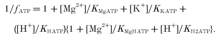(A2)

(A3)

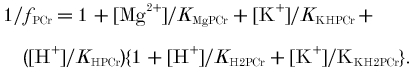(A4)

All these expressions allow for binding of Mg²⁺, K⁺ and two H⁺; eqns (A2) and (A3) also account for simultaneous H⁺ and Mg²⁺ binding, and eqn (A4) allows for simultaneous H⁺ and K⁺ binding. We follow Harkema & Meyer (1997) and Kushmerick (1997) in using dissociation constants throughout (others use dissociation constants for H⁺ and binding (stability) constants for Mg²⁺; Connett, 1988; Roth & Weiner, 1991; Golding et al. 1995). All these f fractions decrease with decreasing pH (Fig. 12B), and so does the ratio that appears in eqn (A1) (Fig. 12D), so that K_CK^app is decreased by acidification.

Adenylate kinase: calculation of AMP

We seek an expression for K_AK^app, the apparent equilibrium constant of the biochemical equation (eqn (2)). We define K_AK^true =[ATP⁴⁻][AMP²⁻]/[ADP³⁻]² as the equilibrium constant of the chemical reaction, which can be taken as 0.363 (Roth & Weiner, 1991) (0.374 in Golding et al. (1995)). Following Roth & Weiner (1991), but using notation based on Harkema & Meyer (1997), we define f_AMP =[AMP³⁻]/[ΣyAMP], so that:

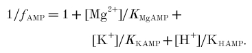(A5)

This allows for binding of Mg²⁺, K⁺ and one H⁺, but neglects binding of a second H⁺ and simultaneous binding of Mg²⁺ and H⁺; comparison with f_ATP above will show how these could be allowed for if desired. Now the apparent equilibrium constant is given by:

(A6)

All three f fractions decrease with decreasing pH (Fig. 12B), but the effects almost cancel, so the ratio that appears in eqn (A6) (Fig. 12D), and thus also K_AK^app, are relatively independent of pH.

atp hydrolysis: calculation of δg_ATP

We define K_ATP^true =[ADP³⁻][HPO₄²⁻]/[ATP⁴⁻] as the equilibrium constant of the chemical reaction of ATP hydrolysis, and K_ATP^app =[ΣADP][ΣP_i]/[ΣATP] as its biochemical equivalent (Golding et al. 1995; Harkema & Meyer, 1997). We take K_ATP^true = 0.0722 (Golding et al. 1995) (0.129 in Harkema & Meyer (1997)), so the standard free energy of ATP hydrolysis (used in eqn (3)) is Δ$G_{\text{ATP}}^0$ = -RTlnK_ATP^app = -32 kJ mol⁻¹ at pH 7. One way to account for the effects of pH on stoichiometry is to correct Δ$G_{\text{ATP}}^0$ using:

(A7)

where f_Pi =[HPO₄²⁻]/[ΣP_i] (i.e. the dianion fraction, to a first approximation 1 - φ). Note that all these f fractions decrease with decreasing pH (Fig. 12B), but the ratio that appears in eqn (A7) increases (Fig. 12D), so Δ$G_{\text{ATP}}^0$ is made less negative by acidification.

Alternatively, as creatine kinase is at equilibrium, the ΔG of ATP hydrolysis must equal that of PCr ‘hydrolysis’, the Lohmann reaction (Harkema & Meyer, 1997). This has the (notional) reactions:

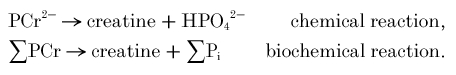Thus a simpler expression for -ΔG_ATP, independent of nucleotide dissociation constants (Harkema & Meyer, 1997), is:

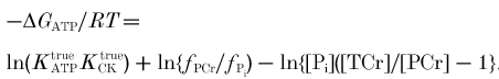(A8)

For this, f_PCr is as given above, and (following Harkema & Meyer (1997) with corrections for K⁺ binding based on Kushmerick (1997)):

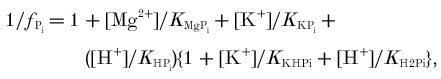(A9)

which allows for binding of H⁺, Mg²⁺, K⁺ and simultaneous H⁺ and K⁺. Both these f fractions decrease with decreasing pH (Fig. 12B), but the ratio that appears in eqn (A8) increases (Fig. 12D), so other things being equal ΔG_ATP is made less negative by acidification.

Relationship to proton stoichiometry of PCr splitting

As well as their implications for the calculation of AMP, ADP and ΔG_ATP (Fig. 2), these considerations are related to the stoichiometry of H⁺ consumption by net PCr splitting (eqn (8)), which is fundamental to this work. Adapting Harkema & Meyer (1997), the stoichiometric coefficient of proton production by the creatine kinase reaction alone (in the direction of ATP synthesis) can be written as a partial derivative:

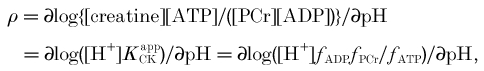which is a negative number, becoming less negative as pH falls (Kushmerick, 1997) (Fig. 12A). By a similar argument, the stoichiometric coefficient for net ATP hydrolysis is:

which is a positive number, decreasing as pH falls (Fig. 12A). Thus for the Lohmann reaction it is the sum of these:

This is dominated by f_Pi. If we ignore Mg²⁺ and K⁺ binding, then f_Pi≈ 1 - φ, and so:

as in the earlier analysis. The more general expression we use (eqn (8)) allows for both Mg²⁺ and K⁺ binding. Both these factors φ and -γ increase in size with decreasing pH (Fig. 12A), and Fig. 12C shows that this is largely due to the pH dependence of the charge on P_i (eqn (A9)); the relatively pH-independent charge on PCr (Fig. 12C) is responsible for the near-constant difference between φ and -γ (Fig. 12A).

As well as these two, another stoichiometric factor has been advocated for analysis of recovery from exercise, where oxidative ATP synthesis results in resynthesis of PCr (Newcomer et al. 1999), and estimating glycolytic rate during exercise (Newcomer & Boska, 1997). In our notation, this factor is 0.85 - (1 - φ) ≈ 0.20 at pH 7; this is close to the factor we use (-γ), and has a similar pH dependence (Fig. 12A). It derives from taking ρ as -0.85 (cf. -0.93 at pH 7 here) and α as (1 - φ) = 0.64 at pH 7 (cf. 0.72 here).

References

- Adams GR, Foley JM, Meyer RA. Muscle buffer capacity estimated from pH changes during rest-to-work transitions. Journal of Applied Physiology. 1990;69:968–972. doi: 10.1152/jappl.1990.69.3.968. [DOI] [PubMed] [Google Scholar]
- Alberty R. Biochemical thermodynamics. Biochimica et Biophysica Acta. 1990;1207:1–11. doi: 10.1016/0167-4838(94)90045-0. [DOI] [PubMed] [Google Scholar]
- Aragon JJ, Tornheim K, Lowenstein JM. On a possible role of IMP in the regulation of phosphorylase activity in skeletal muscle. FEBS Letters. 1980;117:K56–64. doi: 10.1016/0014-5793(80)80570-9. [DOI] [PubMed] [Google Scholar]
- Argov Z, Bank WJ, Maris J, Chance B. Muscle energy metabolism in McArdle's syndrome by in vivo phosphorus magnetic resonance spectroscopy. Neurology. 1987a;37:1720–1724. doi: 10.1212/wnl.37.11.1720. [DOI] [PubMed] [Google Scholar]
- Argov Z, Bank W, Maris J, Leigh J, Chance B. Muscle energy metabolism in human phosphofructokinase deficiency as recorded by 31P nuclear magnetic resonance spectroscopy. Annals of Neurology. 1987b;22:46–51. doi: 10.1002/ana.410220112. [DOI] [PubMed] [Google Scholar]
- Arnold DL, Matthews PM, Radda GK. Metabolic recovery after exercise and the assessment of mitochondrial function in vivo in human skeletal muscle by means of P-31 NMR. Magnetic Resonance in Medicine. 1984;1:307–315. doi: 10.1002/mrm.1910010303. [DOI] [PubMed] [Google Scholar]
- Arthur PG, West TG, Hochachka PW. Quantitative modelling of the effects of selected intracellular metabolites on pH in fish white muscle. Journal of Experimental Biology. 1997;200:1189–1200. doi: 10.1242/jeb.200.8.1189. [DOI] [PubMed] [Google Scholar]
- Austin C, Wray S. An investigation of intrinsic buffering power in rat vascular smooth muscle cells. Pflügers Archiv. 1995;429:325–331. doi: 10.1007/BF00374146. [DOI] [PubMed] [Google Scholar]
- Bangsbo J, Graham T, Johansen L, Strange S, Christensen C, Saltin B. Elevated muscle acidity and energy production during exhaustive exercise in humans. American Journal of Physiology. 1992;263:R891–899. doi: 10.1152/ajpregu.1992.263.4.R891. [DOI] [PubMed] [Google Scholar]
- Bangsbo J, Johansen L, Quistorff B, Saltin B. NMR and analytical evaluation of CrP and nucleotides in the human calf during muscle contraction. Journal of Applied Physiology. 1993;74:2034–2039. doi: 10.1152/jappl.1993.74.4.2034. [DOI] [PubMed] [Google Scholar]
- Bendahan D, Confort-Gouny S, Kozak-Reiss G, Cozzone P. Heterogeneity of metabolic response to muscular exercise in humans. New criteria of invariance defined by in vivo phosphorus-31 NMR spectroscopy. FEBS Letters. 1990;272:155–158. doi: 10.1016/0014-5793(90)80472-u. [DOI] [PubMed] [Google Scholar]
- Bergstrom M, Hultman E. Energy cost and fatigue during intermittent electrical stimulation of human skeletal muscle. Journal of Applied Physiology. 1988;65:1500–1505. doi: 10.1152/jappl.1988.65.4.1500. [DOI] [PubMed] [Google Scholar]
- Blei ML, Conley KE, Kushmerick MJ. Separate measures of ATP utilization and recovery in human skeletal muscle. Journal of Physiology. 1993a;465:203–222. doi: 10.1113/jphysiol.1993.sp019673. erratum: Journal of Physiology (1994) 475 548) [DOI] [PMC free article] [PubMed] [Google Scholar]
- Blei ML, Conley KE, Odderson IB, Esselman PC, Kushmerick MJ. Individual variation in contractile cost and recovery in a human skeletal muscle. Proceedings of the National Academy of Sciences of the USA. 1993b;90:7396–7400. doi: 10.1073/pnas.90.15.7396. [DOI] [PMC free article] [PubMed] [Google Scholar]
- Boska M. Estimating the ATP cost of force production in the human gastrocnemius/soleus muscle group using 31P MRS and 1H MRI. NMR in Biomedicine. 1991;4:173–181. doi: 10.1002/nbm.1940040404. [DOI] [PubMed] [Google Scholar]
- Boska M. ATP production rates as a function of force level in the human gastrocnemius/soleus group using 31P MRS and 1H MRI. Magnetic Resonance in Medicine. 1994;32:1–10. doi: 10.1002/mrm.1910320102. [DOI] [PubMed] [Google Scholar]
- Burton RF. Intracellular buffering. Respiratory Physiology. 1978;33:51–58. doi: 10.1016/0034-5687(78)90083-x. [DOI] [PubMed] [Google Scholar]
- Cady EB, Jones DA, Lynn J, Newham DJ. Changes in force and intracellular metabolites during fatigue of human skeletal muscle. Journal of Physiology. 1989;418:311–325. doi: 10.1113/jphysiol.1989.sp017842. [DOI] [PMC free article] [PubMed] [Google Scholar]
- Chance B, Leigh J, Jr, Clark BJ, Maris J, Kent J, Nioka S, Smith D. Control of oxidative metabolism and oxygen delivery in human skeletal muscle: A steady state analysis of the work/energy cost transfer function. Proceedings of the National Academy of Sciences of the USA. 1985;82:8384–8388. doi: 10.1073/pnas.82.24.8384. [DOI] [PMC free article] [PubMed] [Google Scholar]
- Chasiotis D. The regulation of glycogen phosphorylase and glycogen breakdown in human skeletal muscle. Acta Physiologica Scandinavica. 1983;(suppl. 518):1–68. [PubMed] [Google Scholar]
- Chasiotis D, Bergstrom M, Hultman E. ATP utilization and force during intermittent and continuous contractions. Journal of Applied Physiology. 1987;63:167–174. doi: 10.1152/jappl.1987.63.1.167. [DOI] [PubMed] [Google Scholar]
- Chasiotis D, Sahlin K, Hultman E. Regulation of glycogenolysis in human muscle at rest and during exercise. Journal of Applied Physiology. 1982;53:708–715. doi: 10.1152/jappl.1982.53.3.708. [DOI] [PubMed] [Google Scholar]
- Conley KE, Blei ML, Richards TL, Kushmerick MJ, Jubrias SA. Activation of glycolysis in human muscle in vivo. American Journal of Physiology. 1997;273:C306–315. doi: 10.1152/ajpcell.1997.273.1.C306. erratum: American Journal of Physiology (1997) 276 Ca1) [DOI] [PubMed] [Google Scholar]
- Conley KE, Kushmerick MJ, Jubrias SA. Glycolysis is independent of oxygenation state in stimulated human skeletal muscle in vivo. Journal of Physiology. 1998;511:935–945. doi: 10.1111/j.1469-7793.1998.935bg.x. [DOI] [PMC free article] [PubMed] [Google Scholar]
- Connett R. Analysis of metabolic control: new insights using a scaled creatine model. American Journal of Physiology. 1988;254:R949–959. doi: 10.1152/ajpregu.1988.254.6.R949. [DOI] [PubMed] [Google Scholar]
- Connett R, Gayeski T, Honig C. Energy sources in fully aerobic rest-work transitions: a new role for glycolysis. American Journal of Physiology. 1985;248:H922–929. doi: 10.1152/ajpheart.1985.248.6.H922. [DOI] [PubMed] [Google Scholar]
- Connett RJ. Glycolytic regulation during an aerobic rest-to-work transition in dog gracilis muscle. Journal of Applied Physiology. 1987;63:2366–2374. doi: 10.1152/jappl.1987.63.6.2366. [DOI] [PubMed] [Google Scholar]
- Connett RJ. In vivo control of phosphofructokinase: system models suggest new experimental protocols. American Journal of Physiology. 1989;257:R878–888. doi: 10.1152/ajpregu.1989.257.4.R878. [DOI] [PubMed] [Google Scholar]
- Constantin Teodosiu D, Greenhaff PL, McIntyre DB, Round JM, Jones DA. Anaerobic energy production in human skeletal muscle in intense contraction: a comparison of 31P magnetic resonance spectroscopy and biochemical techniques. Experimental Physiology. 1997;82:593–601. doi: 10.1113/expphysiol.1997.sp004049. [DOI] [PubMed] [Google Scholar]
- Fell DA, Thomas S. Physiological control of metabolic flux: the requirement for multisite modulation. Biochemical Journal. 1995;311:35–39. doi: 10.1042/bj3110035. [DOI] [PMC free article] [PubMed] [Google Scholar]
- Foley JF, Harkema SJ, Meyer RA. Decreased ATP cost of isometric contractions in ATP-depleted rat fast-twitch muscle. American Journal of Physiology. 1991;261:C872–881. doi: 10.1152/ajpcell.1991.261.5.C872. [DOI] [PubMed] [Google Scholar]
- Foley JM, Meyer RA. Energy cost of twitch and tetanic contractions of rat muscle estimated in situ by gated 31P NMR. NMR in Biomedicine. 1993;6:32–38. doi: 10.1002/nbm.1940060106. [DOI] [PubMed] [Google Scholar]
- Funk CI, Clark A, Connett RJ. A simple model of aerobic metabolism: applications to work transitions in muscle. American Journal of Physiology. 1990;258:C995–1005. doi: 10.1152/ajpcell.1990.258.6.C995. [DOI] [PubMed] [Google Scholar]
- Furst P, Josephson B, Vinnars E. Distribution in muscle and liver protein of 15N administered as ammonium acetate to man. Journal of Applied Physiology. 1970;29:307–312. doi: 10.1152/jappl.1970.29.3.307. [DOI] [PubMed] [Google Scholar]
- Garfinkel L, Garfinkel D. Calculation of free-Mg2+ concentration in adenosine 5′-triphosphate containing solutions in vitro and in vivo. Biochemistry. 1984;23:3547–3552. doi: 10.1021/bi00310a025. [DOI] [PubMed] [Google Scholar]
- Golding E, Teague W, Jr, Dobson G. Adjustment of K’ to various pH and pMg for the creatine kinase, adenylate kinase and ATP hydrolysis equilibria permitting quantitative bioenergetic assessment. Journal of Experimental Biology. 1995;198:1775–1782. doi: 10.1242/jeb.198.8.1775. [DOI] [PubMed] [Google Scholar]
- Griffiths JR. A fresh look at glycogenolysis in skeletal muscle. Bioscience Reports. 1981;1:595–610. [Google Scholar]
- Harkema SJ, Adams GR, Meyer RA. Acidosis has no effect on the ATP cost of contraction in cat fast- and slow-twitch skeletal muscles. American Journal of Physiology. 1997;272:C485–490. doi: 10.1152/ajpcell.1997.272.2.C485. [DOI] [PubMed] [Google Scholar]
- Harkema SJ, Meyer RA. Effect of acidosis on control of respiration in skeletal muscle. American Journal of Physiology. 1997;272:C491–500. doi: 10.1152/ajpcell.1997.272.2.C491. [DOI] [PubMed] [Google Scholar]
- Harris RC, Hultman E, Nordesjo L-O. Glycogen, glycolytic intermediates and high-energy phosphates determined in biopsy samples of musculus quadriceps femoris of man at rest. Scandinavian Journal of Laboratory and Clinical Investigation. 1974;33:109–120. [PubMed] [Google Scholar]
- Hochachka PW, Mommsen TP. Protons and anaerobiosis. Science. 1983;219:1391–1397. doi: 10.1126/science.6298937. [DOI] [PubMed] [Google Scholar]
- Hsu A, Dawson M. Accuracy of 1H and 31P MRS analyses of lactate in skeletal muscle. Magnetic Resonance in Medicine. 2000;44:418–426. doi: 10.1002/1522-2594(200009)44:3<418::aid-mrm12>3.0.co;2-g. [DOI] [PubMed] [Google Scholar]
- Hultman E, Spriet LL. Skeletal muscle metabolism, contraction force and glycogen utilization during prolonged electrical stimulation in humans. Journal of Physiology. 1986;374:493–501. doi: 10.1113/jphysiol.1986.sp016093. [DOI] [PMC free article] [PubMed] [Google Scholar]
- Jeneson JAL, Westerhoff HV, Brown TR, van Echteld CJA, Berger R. Quasi-linear relationship between Gibbs free energy of ATP hydrolysis and power-output in human forearm muscle. American Journal of Physiology. 1995;268:C1474–1484. doi: 10.1152/ajpcell.1995.268.6.C1474. [DOI] [PubMed] [Google Scholar]
- Jeneson JAL, Wiseman RW, Westerhoff HV, Kushmerick MJ. The signal transduction function for oxidative phosphorylation is at least second order in ADP. Journal of Biological Chemistry. 1996;271:27995–27998. doi: 10.1074/jbc.271.45.27995. [DOI] [PubMed] [Google Scholar]
- Jouvensal L, Carlier PG, Bloch G. Low visibility of lactate in excised rat muscle using double quantum proton spectroscopy. Magnetic Resonance in Medicine. 1997;38:706–711. doi: 10.1002/mrm.1910380505. [DOI] [PubMed] [Google Scholar]
- Kemp G. Studying metabolic regulation in human muscle. Biochemical Society Transactions. 2000;28:100–103. doi: 10.1042/bst0280100. [DOI] [PubMed] [Google Scholar]
- Kemp GJ. Interactions of mitochondrial ATP synthesis and the creatine kinase equilibrium in skeletal muscle. Journal of Theoretical Biology. 1994;170:239–246. doi: 10.1006/jtbi.1994.1184. [DOI] [PubMed] [Google Scholar]
- Kemp GJ. Physiological constraints on changes in pH and phosphorus metabolite concentrations in ischaemically exercising muscle: implications for metabolic control and for the interpretation of 31P magnetic resonance spectroscopy studies. Magnetic Resonance Materials in Physics, Biology and Medicine. 1997;5:231–241. doi: 10.1007/BF02594586. [DOI] [PubMed] [Google Scholar]
- Kemp GJ, Manners DN, Bastin ME, Clark JF, Radda GK. A theoretical model of the mitochondrion/creatine kinase/myofibril system in muscle. Molecular and Cellular Biochemistry. 1998;184:249–289. [PubMed] [Google Scholar]
- Kemp GJ, Radda GK. Quantitative interpretation of bioenergetic data from 31P and 1H magnetic resonance spectroscopic studies of skeletal muscle: an analytical review. Magnetic Resonance Quarterly. 1994;10:43–63. [PubMed] [Google Scholar]
- Kemp GJ, Sanderson AL, Thompson CH, Radda GK. Regulation of oxidative and glycogenolytic ATP synthesis in exercising rat skeletal muscle. NMR in Biomedicine. 1996;9:261–270. doi: 10.1002/(SICI)1099-1492(199609)9:6<261::AID-NBM430>3.0.CO;2-B. [DOI] [PubMed] [Google Scholar]
- Kemp GJ, Taylor DJ, Styles P, Radda GK. The production, buffering and efflux of protons in human skeletal muscle during exercise and recovery. NMR in Biomedicine. 1993;6:73–83. doi: 10.1002/nbm.1940060112. [DOI] [PubMed] [Google Scholar]
- Kemp GJ, Thompson CH, Barnes PRJ, Radda GK. Comparisons of ATP turnover in human muscle during ischaemic and aerobic exercise using 31P magnetic resonance spectroscopy. Magnetic Resonance in Medicine. 1994;31:248–258. doi: 10.1002/mrm.1910310303. [DOI] [PubMed] [Google Scholar]
- Korzeniewski B. Regulation of ATP supply during muscle contraction: theoretical studies. Biochemical Journal. 1998;330:1189–1195. doi: 10.1042/bj3301189. [DOI] [PMC free article] [PubMed] [Google Scholar]
- Kushmerick MJ. Multiple equilibria of cations with metabolites in muscle bioenergetics. American Journal of Physiology. 1997;272:C1739–1747. doi: 10.1152/ajpcell.1997.272.5.C1739. [DOI] [PubMed] [Google Scholar]
- Kushmerick MJ. Energy balance in muscle activity: simulations of ATPase coupled to oxidative phosphorylation and to creatine kinase. Comparative Biochemistry and Physiology B: Biochemistry and Molecular Biology. 1998;120:109–123. doi: 10.1016/s0305-0491(98)00026-1. [DOI] [PubMed] [Google Scholar]
- Mahler M. First-order kinetics of muscle oxygen consumption, and an equivalent proportionality between QO2 and phosphorylcreatine level. Journal of General Physiology. 1985;86:135–165. doi: 10.1085/jgp.86.1.135. [DOI] [PMC free article] [PubMed] [Google Scholar]
- Mainwood GW, Renaud JM. The effect of acid-base balance on fatigue of skeletal muscle. Canadian Journal of Physiology and Pharmacology. 1985;63:403–416. doi: 10.1139/y85-072. [DOI] [PubMed] [Google Scholar]
- Mannion AF, Jakeman PM, Dunnett M, Harris RC, Willan PL. Carnosine and anserine concentrations in the quadriceps femoris muscle of healthy humans. European Journal of Applied Physiology. 1992;64:47–50. doi: 10.1007/BF00376439. [DOI] [PubMed] [Google Scholar]
- Mannion AF, Jakeman PM, Willan PL. Determination of human skeletal muscle buffer value by homogenate technique: methods of measurement. Journal of Applied Physiology. 1993;75:1412–1418. doi: 10.1152/jappl.1993.75.3.1412. [DOI] [PubMed] [Google Scholar]
- Masuda T, Dobson GP, Veech RL. The Gibbs-Donnan near-equilibrium system of heart. Journal of Biological Chemistry. 1990;256:20321–20334. [PubMed] [Google Scholar]
- Mazzeo A, Levy G. An evaluation of new processing protocols for in vivo NMR spectroscopy. Magnetic Resonance in Medicine. 1991;17:483–495. doi: 10.1002/mrm.1910170219. [DOI] [PubMed] [Google Scholar]
- Meyer RA. A linear model of muscle respiration explains monoexponential phosphocreatine changes. American Journal of Physiology. 1988;254:C548–553. doi: 10.1152/ajpcell.1988.254.4.C548. [DOI] [PubMed] [Google Scholar]
- Meyer RA, Sweeney HL, Kushmerick MJ. A simple analysis of the "phosphocreatine shuttle". American Journal of Physiology. 1984;246:C365–377. doi: 10.1152/ajpcell.1984.246.5.C365. [DOI] [PubMed] [Google Scholar]
- Miller R, Boska M, Moussavi R, Carson P, Weiner M. 31P Nuclear magnetic resonance studies of high energy phosphates and pH in human muscle fatigue. Journal of Clinical Investigation. 1988;81:1190–1196. doi: 10.1172/JCI113434. [DOI] [PMC free article] [PubMed] [Google Scholar]
- Moon R, Richards J. Determination of the intracellular pH by 31P magnetic resonance. Journal of Biological Chemistry. 1973;248:7276–7278. [PubMed] [Google Scholar]
- Nevill ME, Boobis LH, Brooks SA, Williams C. Effect of training on muscle metabolism during treadmill sprinting. Journal of Applied Physiology. 1989;67:2376–2382. doi: 10.1152/jappl.1989.67.6.2376. [DOI] [PubMed] [Google Scholar]
- Newcomer BR, Boska MD. Adenosine triphosphate production rates, metabolic economy calculations, pH, phosphomonoesters, phosphodiesters, and force output during short-duration maximal isometric plantar flexion exercises and repeated maximal isometric plantar flexion exercises. Muscle and Nerve. 1997;20:336–346. doi: 10.1002/(SICI)1097-4598(199703)20:3<336::AID-MUS11>3.0.CO;2-Z. [DOI] [PubMed] [Google Scholar]
- Newcomer BR, Boska MD, Hetherington HP. Non-Pi buffer capacity and initial phosphocreatine breakdown and resynthesis kinetics of human gastrocnemius/soleus muscle groups using 0. 5 s time-resolved 31P MRS at 4.1 T. NMR in Biomedicine. 1999;12:545–551. doi: 10.1002/(sici)1099-1492(199912)12:8<545::aid-nbm595>3.0.co;2-j. [DOI] [PubMed] [Google Scholar]
- Newham DJ, Jones DA, Turner DL, McIntyre D. The metabolic costs of different types of contractile activity of the human adductor pollicis muscle. Journal of Physiology. 1995;488:815–819. doi: 10.1113/jphysiol.1995.sp021013. [DOI] [PMC free article] [PubMed] [Google Scholar]
- Paganini AT, Foley JM, Meyer RA. Linear dependence of muscle phosphocreatine kinetics on oxidative capacity. American Journal of Physiology. 1997;272:C501–510. doi: 10.1152/ajpcell.1997.272.2.C501. [DOI] [PubMed] [Google Scholar]
- Pan JW, Hamm JR, Hetherington HP, Rothman DL, Shulman RG. Correlation of lactate and pH in human skeletal muscle after exercise by 1H NMR. Magnetic Resonance in Medicine. 1991;20:57–65. doi: 10.1002/mrm.1910200107. [DOI] [PubMed] [Google Scholar]
- Parkhouse WS, McKenzie DC. Possible contribution of skeletal muscle buffers to enhanced anaerobic performance: a brief review. Medical Science in Sports and Exercise. 1984;16:328–338. [PubMed] [Google Scholar]
- Putman CT, Spriet LL, Hultman E, Dyck DJ, Heigenhauser GJ. Skeletal muscle pyruvate dehydrogenase activity during acetate infusion in humans. American Journal of Physiology. 1995;268:E1007–1017. doi: 10.1152/ajpendo.1995.268.5.E1007. [DOI] [PubMed] [Google Scholar]
- Ren JM, Hultman E. Regulation of glycogenolysis in human skeletal muscle. Journal of Applied Physiology. 1989;67:2243–2248. doi: 10.1152/jappl.1989.67.6.2243. [DOI] [PubMed] [Google Scholar]
- Ren JM, Hultman E. Regulation of phosphorylase a activity in human skeletal muscle. Journal of Applied Physiology. 1990;69:919–923. doi: 10.1152/jappl.1990.69.3.919. [DOI] [PubMed] [Google Scholar]
- Roos A, Boron WF. Intracellular pH. Physiological Reviews. 1981;61:296–434. doi: 10.1152/physrev.1981.61.2.296. [DOI] [PubMed] [Google Scholar]
- Roth K, Weiner MW. Determination of cytosolic ADP and AMP concentrations and the free energy of ATP hydrolysis in human muscle and brain tissues with 31P NMR spectroscopy. Magnetic Resonance in Medicine. 1991;22:505–511. doi: 10.1002/mrm.1910220258. erratum in Magnetic Resonance in Medicine (1995) 33 282) [DOI] [PubMed] [Google Scholar]
- Roussel M, Kemp G, Bendahan D, Le Fur Y, Cozzone P. Magnetic Resonance Materials in Physics, Biology and Medicine 1998. suppl. 1. Vol. 6. Geneva, Switzerland: 1998. A 31P MRS study of ATP synthesis and proton handling in ischaemic exercise; p. 237. [Google Scholar]
- Roussel M, Kemp G, Bendahan D, Le Fur Y, Cozzone P. Philadelphia, USA: 1999. Regulation of ATP synthesis and proton handling during ischaemic exercise; p. 696. 7th Annual Meeting of the Society for Magnetic Resonance, May 22–28, 1999. [Google Scholar]
- Sahlin K. Intracellular pH and energy metabolism in skeletal muscle of man. Acta Physiologica Scandinavica. 1978;(suppl. 455):1–56. [PubMed] [Google Scholar]
- Sahlin K, Alvestrand A, Brandt R, Hultman E. Intracellular pH and bicarbonate concentration in human skeletal muscle during recovery from exercise. Journal of Applied Physiology. 1978;45:474–480. doi: 10.1152/jappl.1978.45.3.474. [DOI] [PubMed] [Google Scholar]
- Sahlin K, Henriksson J. Buffer capacity and lactate accumulation in skeletal muscle of trained and untrained men. Acta Physiologica Scandinavica. 1984;122:331–339. doi: 10.1111/j.1748-1716.1984.tb07517.x. [DOI] [PubMed] [Google Scholar]
- Spriet LL, Soderlund K, Bergstrom M, Hultman E. Anaerobic energy release in skeletal muscle during electrical stimulation in men. Journal of Applied Physiology. 1987a;62:611–615. doi: 10.1152/jappl.1987.62.2.611. [DOI] [PubMed] [Google Scholar]
- Spriet LL, Soderlund K, Bergstrom M, Hultman E. Skeletal muscle glycogenolysis, glycolysis, and pH during electrical stimulation in men. Journal of Applied Physiology. 1987b;62:616–621. doi: 10.1152/jappl.1987.62.2.616. [DOI] [PubMed] [Google Scholar]
- Spriet LL, Soderlund K, Hultman E. Energy cost and metabolic regulation during intermittent and continuous tetanic contractions in human skeletal muscle. Canadian Journal of Physiology and Pharmacology. 1988;66:134–139. doi: 10.1139/y88-024. [DOI] [PubMed] [Google Scholar]
- Sullivan MJ, Saltin B, Negro Vilar R, Duscha BD, Charles HC. Skeletal muscle pH assessed by biochemical and 31P-MRS methods during exercise and recovery in men. Journal of Applied Physiology. 1994;77:2194–2200. doi: 10.1152/jappl.1994.77.5.2194. [DOI] [PubMed] [Google Scholar]
- Teague WE, Jr, Golding EM, Dobson GP. Adjustment of K’ for the creatine kinase, adenylate kinase and ATP hydrolysis equilibria to varying temperature and ionic strength. Journal of Experimental Biology. 1996;199:509–512. doi: 10.1242/jeb.199.2.509. [DOI] [PubMed] [Google Scholar]
- Veech RL, Lawson JWR, Cornell NW, Krebs HA. Cytosolic phosphorylation potential. Journal of Biological Chemistry. 1979;254:6538–6547. [PubMed] [Google Scholar]
- Vezzoli A, Gussoni M, Greco F, Zetta L, Cerretelli P. Quantitative analysis of anaerobic metabolism in resting anoxic muscle by 31P and 1H MRS. Biochimica et Biophysica Acta. 1997;1322:195–207. doi: 10.1016/s0005-2728(97)00070-4. [DOI] [PubMed] [Google Scholar]
- Wackerhage H, Mueller K, Hoffmann U, Leyk D, Essfeld D, Zange J. Glycolytic ATP production estimated from 31P magnetic resonance spectroscopy measurements during ischemic exercise in vivo. Magnetic Resonance Materials in Physics, Biology and Medicine. 1996;4:151–155. doi: 10.1007/BF01772002. [DOI] [PubMed] [Google Scholar]
- Walter G, Vandenborne K, Elliot M, Leigh J. In vivo ATP synthesis rates in single human muscles during high intensity exercise. Journal of Physiology. 1999;519:901–970. doi: 10.1111/j.1469-7793.1999.0901n.x. [DOI] [PMC free article] [PubMed] [Google Scholar]
- Westerhoff HV, van Echteld CJ, Jeneson JA. On the expected relationship between Gibbs energy of ATP hydrolysis and muscle performance. Biophysical Chemistry. 1995;54:137–142. doi: 10.1016/0301-4622(94)00129-8. [DOI] [PubMed] [Google Scholar]
- Wolfe CL, Gilbert HF, Brindle KM, Radda GK. Determination of buffering capacity of rat myocardium during ischaemia. Biochimica et Biophysica Acta. 1988;971:9–20. doi: 10.1016/0167-4889(88)90156-5. [DOI] [PubMed] [Google Scholar]
- Yamada T, Kikuchi K, Sugi H. 31P nuclear magnetic resonance studies on the glycogenolysis regulation in resting and contracting frog skeletal muscle. Journal of Physiology. 1993;460:273–286. doi: 10.1113/jphysiol.1993.sp019471. [DOI] [PMC free article] [PubMed] [Google Scholar]