Effect of genetic divergence in identifying ancestral origin using HAPAA

Abstract

The genome of an admixed individual with ancestors from isolated populations is a mosaic of chromosomal blocks, each following the statistical properties of variation seen in those populations. By analyzing polymorphisms in the admixed individual against those seen in representatives from the populations, we can infer the ancestral source of the individual’s haploblocks. In this paper we describe a novel approach for ancestry inference, HAPAA (HMM-based analysis of polymorphisms in admixed ancestries), that models the allelic and haplotypic variation in the populations and captures the signal of correlation due to linkage disequilibrium, resulting in greatly improved accuracy. We also introduce a methodology for evaluating the effect of genetic divergence between ancestral populations and time-to-admixture on inference accuracy. Using HAPAA, we explore the limits of ancestry inference in closely related populations.

Human population migration, adaptation, and admixture have a chaotic and mostly undocumented history. However, nature has auspiciously recorded its account of events within our genomes, and we are at the cusp of an era where we will be able to unlock these records. An individual’s genome is a mosaic of ancestral haploblocks whose sizes depend on how far back in the ancestry we compare them. Because recombination can occur essentially anywhere in the genome, the precise boundaries and sources of these haploblocks cannot be easily inferred. However, if the haploblocks are derived from isolated human subpopulations, they will tend to follow the patterns of variation seen in those populations. Using these patterns, we can partition an admixed individual’s genome into a mosaic of blocks derived from different populations. The inference of admixed ancestries is intriguing from a personal perspective because it speaks to an individual’s origins. In addition, it can be used in association mapping studies to identify loci relevant in genetic disease (McKeigue 1998; Hoggart et al. 2004; Montana and Pritchard 2004; Patterson et al. 2004; Zhu et al. 2004, 2005) and will help unravel some of the complexities in the history of human evolution.

Although recent work suggests that human genomes differ significantly in many ways (Redon et al. 2006), single nucleotide polymorphisms (SNPs) are ubiquitous and can serve as markers for the variation. Recent advances in genotyping technology allow us to genotype hundreds of thousands of SNPs in a single experiment, making them a convenient vehicle for studying genome-wide variation. For example, the Illumina HumanHap550 genotyping chip can assay over 550,000 tag-SNP loci for a few hundred dollars (http://illumina.com/pages.ilmn?ID=154). Because linkage disequilibrium (LD) has a strong effect at short genetic distances, the high-density coverage of such genotyping chips makes it possible to infer much of the intervening genomic variation (Carlson et al. 2004). Using SNPs as a basis for variation, methods have been described recently that infer the ancestral population composition of admixed individuals, known as the ancestral haploblock reconstruction or inference problem. These methods are often probabilistic models that use the statistical properties of alleles seen in different populations to derive the most likely ancestral origin of each locus. For example, some methods use a first-order hidden Markov model (HMM) whose hidden states each correspond to an ancestral population (Falush et al. 2003; Hoggart et al. 2004; Patterson et al. 2004; Zhu et al. 2004). Other methods use more complex models that account for some amount of LD between loci (Tang et al. 2006). Here, we present two main contributions: (1) HAPAA (HMM-based analysis of polymorphisms in admixed ancestries), a novel approach for ancestral haploblock inference that is more accurate than previous methods (http://hapaa.stanford.edu); and (2) a methodology that studies the limitations of inference as a function of both the genetic similarity between ancestral populations and the number of generations since first admixture between those populations. Unlike other methods, our inference methodology models long-range allelic correlations due to LD via a representation that makes explicit the haplotypes seen in different populations. By conducting large simulations of population evolution, we are able to test the dependence of population divergence on ancestry inference. In contrast, tests done in the past have relied on a few specific populations with fixed divergence, for example the four in the HapMap data set (International HapMap Consortium 2005). Together, our study allows us to better understand the limitations of genomic analysis in decoding an individual’s history of admixture.

In Methods, we summarize the ancestral haploblock inference problem in technical detail, review some previous inference methodologies, and finally describe the HAPAA method. In Results, we first compare the performance of HAPAA to the best previous method, and then study the effect of population genetic divergence on ancestry inference. Finally, we describe our experiments in varying the input to our methodology and show that it is robust to changes in representing the populations.

Methods

Problem formulation

Suppose we have N populations P = {P₁, P₂, . . . , P_N}, each represented by a set of n_p model individuals P_p = {a_p1, a_p2, . . . , a_pnp}. For each individual a_pk we have SNP genotypes sampled at L loci spaced across the genome, phased into two putative haplotypes a_pk0 = 〈a_pk01, a_pk02, . . . , a_pk0L〉 and a_pk1, where at each locus we have a_pkhi ∈ {A, C, G, T, −}. We assume that the per-generation probability of recombination (the genetic distance) between any two adjacent loci i and (i + 1) is known to be R_i for all populations.

Given a new, potentially admixed individual genotyped at the same loci a^g = 〈, , . . . , 〉, we would like to determine the unobserved, true ancestral origin of each locus in the two haplotypes z^m = 〈, , . . . , 〉 (maternally derived) and z_f (paternal), where the ancestral origin is confined to one of the given populations , ∈ {1, . . . , N}. Thus, the problem of ancestral haploblock reconstruction can be seen as using a set of model individuals representing the populations P and observed SNP genotypes a^g to infer the “most likely” ancestral assignment ∈ {1, . . . , N} and .

For simplicity, let us begin by assuming that we know the true phasing of the individual, so that we can do inference on each haplotype independently. The problem thus reduces to assigning an ancestral origin to each SNP locus z_i ∈ {1, . . . , N} from a haplotype of alleles a_i ∈ {A, C, G, T, −}. After we have solved this problem, we will extend our solution to unphased genotypes.

Previous work

Existing approaches vary considerably; our work follows methods that model SNPs as the successive emissions of a probabilistic graphical model (Falush et al. 2003; Hoggart et al. 2004; Patterson et al. 2004; Zhu et al. 2004). The model allows us to perform inference on a set of hidden states {S₁, S₂, . . . , S_N}, each corresponding to one of the N ancestral populations. Transitions between the populations as we move along the genome are governed by a Markov process. In a population state S_p, the model probabilistically emits alleles based on the frequencies seen in the model individuals in P_p. An example of emission probabilities for a first-order HMM is P(a_i = x|z_i = S_p) = (1/2n_p) 1[a_pkhi = x] where 1[condition] ∈ {0, 1} is the indicator function and x ∈ {A, C, G, T, −}. The method used in SABER (Tang et al. 2006) improved on this by emitting alleles according to pair-allele frequencies P(a_i = x| = S_p, a_i−1). The probability of transitioning states P(z_i+1 = S_p′|z_i = S_p) between two loci i and (i + 1) depends on the genetic distance between the loci R_i and genome-wide model parameters τ_p, the time since admixing for chromosome blocks derived from population p, which are learned from examples. The state diagram is depicted in Figure 1B.

Figure 1.

(A) Hierarchical HMM state diagram for HAPAA. On the left, inter- and intra-population transitions occur with probabilities governed by matrix A(p, p′). In the middle, each population P_p has a similar structure: entry state In_p transitions with uniform probability to a diploid model individual a_pk, then to exit state Out_p. On the right, in a_pk we transition into one of two states representing the haplotypes S_pk0 and S_pk1 of model individual a_pk with equal probability. Each haplotype emits its alleles a_pkhi via a mutation/error probability distribution M(a^pkhi, a_i). Haplotypes transition to each other with probability proportional to the phase switch error W_pki, and transition out of the diploid sample with probability governed by genetic distance to the next locus R_i and the population-specific recombination rate parameter τ_p. (B) HMM state diagram for previous methods. Each state represents a population and emits alleles according to frequency estimates for the populations, and admixture transition probabilities depend on the degree of admixture expected and other learned parameters. By construction, these methods assume a greater degree of independence between adjacent loci.

Although SABER attempts to address the problem via a second-order model, fixed-order models do not fully exploit the information available by examining the full haplotypes in the model individuals. Even though it is possible to further expand on SABER by devising a third-order or fourth-order model, the size of these models grows exponentially and becomes intractable to learn.

HAPAA methodology

The model

To capture the effects of linkage disequilibrium at larger distances, our methodology uses a representation of possible emissions that models long-range correlations between alleles in haplotypes. The HMM, depicted in Figure 1A, has an emitting state S_pkh for the two haplotypes h ∈ {0, 1} of each model individual k in population p. In addition, there are non-emitting states {In_p} and {Out_p} for each population p, that serve as the primary means of transitioning between haplotypes {S_pkh}. If the hidden state variable is denoted y_i, the probability of emission is given by the 5 × 5 matrix P(a_i = x|y_i = S_pkh) = M(a_pkhi, x). Here, M(x, x) is typically very likely, while M(x′, x ≠ x′) provides a small allowance for haplotypes not seen in the representative individuals, mutations, and genotyping error.

Our HMM starts in an emitting state with equal probability for each population given by P(y₁ = S_pkh) = 1/2Nn_p. Each state S_pkh can transition to three places: back to itself with probability (1 − w^pki)e^−τ_pR_i, to the other putative haplotype within the same model individual S_pk(1−h) with probability w^pki ⋅ e^−τ_pR_i, or to the exit state Out_p with probability 1 − e^−τ_pR_i. The recombination rate parameters τ_p are learned from training examples and can be interpreted as the reciprocal of the expected genetic length of a haploblock inherited from population p. The constants w_pki represent the probability of a phasing switch error between loci i and (i + 1) for model individual k in population p. In the ideal situation with no phasing errors, we set w_pki = 0, in which case we will never transition directly between the two putative haplotypes of an individual. The other way of transitioning between haploblocks is from S_pkh to an Out_p state, then to an In_p′ state with probability specified by the N × N admixture matrix P(Out^p → In_p′) = A(p, p′), and finally back to an emitting haplotype state S_p′k′h′ with uniform probability 1/2n_p′. Note that, in order to switch between haploblocks within the same population p, we still transition to Out_p and then In_p with probability A(p, p). This hierarchical structure of our HMM is depicted in Figure 1A.

Inference and testing

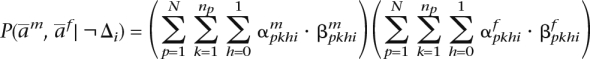
We infer the ancestral origins z_i by first computing the standard forward α_pkhi, backward β_pkhi, and posterior probability matrices γ_pkhi (Durbin et al. 1998). We then compute the population-total posterior probability Γ_pi = γ_pkhi and finally set zⁱ = argmax^pΓ_pi, the population with maximal total posterior probability.

In order to reduce the occurrence of false positives, we then apply a filtering procedure with a single parameter, the genetic length of the minimum acceptable block size ε. We partition z_i into the largest consecutive blocks {ζ_j} of equal ancestry assignments. Every block that is larger than ε is marked “solid”, and for each remaining smaller block ζ_j we find the population of the last preceding solid block pop_L(ζ_j) (if it exists) and the population of the first subsequent solid block pop_R(ζ_j). Next, we recompute the forward, backward, and posterior matrices with additional constraints: (1) for each solid block ζ_j, we force the emitting states to be in population, pop(ζ_j), and (2) for each small block ζ_j, we force the emitting states to be in either population pop_L(ζ_j) or population pop_R(ζ_j), and the only A(p, p′) transitions allowed are from pop_L(ζ_j) or pop_R(ζ_j) back to themselves, or one-way from pop_L{ζ_j} to pop_R(ζ_j). Finally, we once again infer z_i as described above.

To test our model, ideally we would use real, labeled, admixed individuals. Such data may become available in the future, but for now we synthesize test individuals using a model that we believe more closely reflects the properties of recombination. We construct a G^th generation admixed individual by selecting 2^G (potentially redundant) ancestors from individuals left out for test set construction and simulating the mating process over G generations. For each chromosome, the number of recombination points is chosen from a normal distribution with mean equal to the chromosome’s genetic length, with a minimum of one crossover per meiosis. The result is an admixed individual where each locus is annotated with its source population.

Training

From the above description, our model consists of the following parameters: the emission probability matrix M(x′, x), the recombination rates τ_p, and the admixture transition matrix A(p, p′). We perform supervised learning of these parameters using an EM algorithm on training examples (Durbin et al. 1998). The examples are labeled with their true ancestral origins z_i, and we constrain the HMM so that if z_i = p then y_i = S_pkh for some k and h, restricting ourselves to model haplotypes within the true population. Our filtering procedure adds an additional parameter ε, which we train by maximizing one of our scoring metrics (described later in the paper) via a grid-search method.

When real admixed training examples are not available, it is still possible to train using simulated admixed examples constructed from the model individuals themselves, while at the same time avoiding overfitting. For all our experiments, we synthesize training examples from the model individuals using the same procedure described above for the generation of admixed test individuals. The result is a synthetic admixed haplotype ã_i, where, at each locus i, an allele can be annotated with the model haplotype from which it is derived: = 〈p, k, h〉 indicates that locus i is derived from model individual k haplotype h of population p. When training on ã, we constrain the HMM so that at each locus i it is not allowed to be in the state corresponding to its source haplotype: yⁱ ≠ , forcing it to model the training example using the remaining model individuals.

Extension to genotypes

Earlier we assumed that we knew the true phasing of a^g, but typically we would be presented with unphased genotypes a^g = 〈, , . . . , 〉. We extend our method to genotypes using the following iterative procedure.

Initialization

Based on the precomputed haplotypes of the model individuals a_pkh, construct an initial phasing of the genotypes of a^g into two halotypes a^m = 〈, , . . . , 〉 and a^f using a program such as HAP (Halperin and Eskin 2004), PHASE (Stephens et al. 2001), fastPHASE (Scheet and Stephens 2006), or an algorithm we developed that is significantly faster at the expense of a marginal performance decrease (not described here). Between each pair of consecutive loci we describe the likelihood of a phase switch between the two haplotypes with a vector w_i, the probability of a phase switch between loci i and (i + 1). For phasing methods that do not estimate this directly, we set the vector to a uniform switch probability between heterozygous locations.

Iterative step

Compute the forward and backward matrices using our HMM on each haplotype independently, producing and for the putative maternal haplotype, and and for the paternal. Given the current phasing, we use our HMM model to compute the probability of witnessing these two haplotypes for any locus i as

where Δ_i is the event that there is a phase switch error between locus i and (i + 1).

Suppose now that the haplotypes had exactly one phase switch error between locus i and (i + 1). Then, we could compute the probability of witnessing the two haplotypes as:

Using the vector w_i as a prior for the phase switch at i, we can use Bayes’ rule to compute

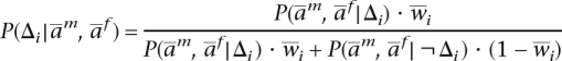We compute this conditional probability for each locus and heuristically pick a set of loci H with the following procedure:

1. Find h = argmax_i P(Δ_i|a^m, a^f). If this probability is >1/2 then add h to H, otherwise stop.

2. Find maximum h^L < h such that wⁱ > 2 and minimum h^R > h such that wⁱ > 2. Exclude the range [h_L, h_R] from further consideration and repeat step 1.

The limit of 2 was chosen to avoid selecting multiple nearby loci that stem from a single phase switch error. If the set H is empty, then we terminate the iterative procedure. Otherwise, we update the two haplotypes a^m and a^f by switching the phase at each locus in H and repeat the iterative step, not allowing the same loci in H to be picked again. Empirically, this procedure terminates after seven to 20 iterations.

Finalization

Compute the posterior probabilities for the two haplotypes and , the population-total posteriors and , and finally decode the inferred ancestries and .

All tests in Results were conducted on unphased genotypes using this methodology.

Results

Comparison to previous work

We benchmarked HAPAA against the current best-performing method, the Markov-HMM-based SABER (Tang et al. 2006). We used the HapMap data set (International HapMap Consortium 2005), representing three populations: 60 unrelated North-Western Europeans (CEU), 60 Yoruban-Africans (YRI), and 90 East Asians (ASN = CHB [Han Chinese] + JPT [Japanese]). We restricted the data set to the loci in the Illumina HumanHap550 genotyping chip (http://illumina.com/pages.ilmn?ID=154) within chromosome 22, spaced 4.5 kb apart on average, and used a recombination rate map computed from HapMap (McVean et al. 2004; Winckler et al. 2005). We partitioned each population into two sets of individuals: 5/6 for the model individuals and for training, and 1/6 for test set construction. Our test set comprised 400 individuals, consisting of 20 simulated diploid genotypes for each value of G ∈ {1, 2, . . . , 20}, which we phased using our own algorithm. Each test individual was derived by simulating the mating process over G generations, beginning with 2^G ancestral individuals drawn with equal probability from each of the three populations. We constructed a training set in a similar fashion, picking ancestors from the model individuals instead, at the same time avoiding overfitting via the technique described in Methods for training HAPAA. We trained a single set of model parameters for all tests using our EM algorithm and optimized the filtering procedure by maximizing the accuracy of ancestry recall.

To measure the performance of the two methods, we used the mean-square-error metric (Tang et al. 2006),

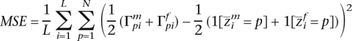where each of the maternal and paternal haplotypes contributes 1/2 to the measure. Figure 2 is a demonstration of results produced at different stages of inference by HAPAA compared to those by SABER. The performance comparison in Figure 3 shows that HAPAA’s inference is significantly more accurate, though there is a clear correlation between the methods. Because HAPAA relies on inferring a phasing of genotypes into two haplotypes, we found that for G = 1, where entire chromosomes come from the same ancestry, phasing errors impair our performance compared to SABER. As the number of generations G increases, the problem of inferring the recombinations between ancestries dominates the problem of determining phase. However, HAPAA manages to infer the ancestral origin with higher fidelity than SABER by better modeling the effects of linkage disequilibrium in each population. As G approaches 20, the errors appear to level off as the distribution of expected haploblock sizes remains relatively stable.

Figure 2.

Example inference on chromosome 22 of an individual admixed between three HapMap populations. The top two tracks represent the true ancestries, followed by three stages of HAPAA processing, and finally posterior probabilities and Viterbi decoding by SABER. The gray bars highlight two locations with correctly inferred ancestry but with phase switching errors between the haplotypes.

Figure 3.

Performance comparison between HAPAA and SABER. We measured the mean-square-error of the inferred posterior probability of population ancestry on chromosome 22 for a varying number of generations of admixture. Tests were constructed by simulating admixture over G generations from 2^G individuals selected randomly from three HapMap populations.

Effect of genetic divergence on inference

Although the HapMap data set is useful for some basic validation, it is somewhat limiting for the purpose of studying the problem of ancestral inference. The genetic divergences between the four populations exemplify two extremes of the problem: Distinguishing between haploblocks derived from CEU and YRI is relatively straightforward, while haploblocks from CHB and JPT are virtually indistinguishable. To better assess the performance of ancestry inference we created a novel testing methodology that measures performance as a function of the genetic distance between populations.

First, we construct pairs of populations separated by D ∈ {100, 200, . . . , 2000} generations via simulation: Starting with the whole-genome HapMap CEU population restricted to the Illumina 550K sites, we simulate the divergence of two populations over the course of D generations of random mating with fixed population sizes of 5000. The results have a strong dependence on this parameter—we chose it to be between the effective population sizes of 3100 and 7500 estimated by Tenesa et al. (2007). Other numbers for the effective human population size exist, but we chose this estimate specifically because it was based on the HapMap data set. Although we simulate recombination and genetic drift, we do not model selection or novel mutations, which would tend to make the populations more divergent and the ancestry inference problem easier. Other models incorporating effects such as continuous gene flow may also affect the divergence. However, since human population history is sufficiently complex that there is no consensus on the most accurate model, we have chosen to use a simple, reasonable one. We randomly divide each population into a model/training partition consisting of 60 individuals and the remainder for test set construction.

For this data set, we measure the ability of our inference algorithm to recall a trace amount of ancestry from one population in a background of the other population. For example, suppose an individual’s ancestors G generations ago consisted of 2^G − 1 individuals from population A and only one individual from population B. This methodology is illustrated in Figure 4. Testing different values of G ∈ {1, 2, . . . , 20} and conditioned on the event that there exists some remaining ancestry derived from the minor population B, we measured our ability to detect the signal from the minor population. We report on our recall = true positives/(true positives + false negatives) and precision = true positives/(true positives + false positives) for correctly assigning the minor ancestry to each locus and .

Figure 4.

Methodology for studying the effect of genetic divergence on ancestry inference. We simulate pairs of randomly mating populations of fixed size 5000 derived from the HapMap CEU population over D generations. We construct training and test individuals derived over G generations of admixture from 2^G − 1 ancestors from one population and one ancestor from the other (minor) population.

To train our parameters, we constructed 2000 simulated training genomes from the model individuals for each pair of populations parameterized by the number of generations of divergence D. We trained our model using EM and optimized our filtering procedure by maximizing the product of the recall and precision measure. We benchmarked the performance on a test set that consisted of 100 admixed individuals derived from the test partition for each D and G, for a total of 40,000 full-genome inferences, and plot the results in Figure 5.

Figure 5.

Recall and precision of detecting minor population. We simulated 20 pairs of populations separated by D ∈ {100, 200, . . . , 2000} generations of drift on the whole genome of Illumina 550K loci. For each D we constructed test individuals that were derived over G ∈ {1, 2, . . . , 20} generations of admixture from 2^G − 1 ancestors from one population and one ancestor from the other (minor) population. Conditioned on the existence of at least one haploblock derived from the minor population, we measure the ability of HAPAA to identify these loci.

It is clear that both genetic distance between populations and generations of admixture significantly affect the accuracy of inference. For populations that are not very divergent (D = 100), it is possible to infer the ancestry of very recent admixture (G ≤ 2). However, as we increase the number of generations of admixture, there is not enough divergence between the populations to correctly classify the haploblocks. In the other extreme, for populations that have been reproductively isolated by many generations (D = 2000), inference is possible with high recall and precision. From our simulations, even with G = 10 generations of admixture, HAPAA is able to detect the presence of haploblocks inherited from one individual in the minor population among haploblocks derived from 2^G − 1 ancestors in the other population. As our genomes recombine over a large number of generations, most ancestral haploblocks will disappear. However, we estimate that even a 10th-generation ancestor has a significant probability of 26% of having a remaining haploblock. Therefore, for many individuals with ancestry admixed within 10 generations, we anticipate being able to detect the presence of both populations.

Varying the number of model individuals

Unlike profile-HMM approaches or the Markov-HMM of SABER, in HAPAA each model individual haplotype is a separate state in the HMM. To understand how the number of model individuals affects performance, we performed the following two experiments.

Uniform population size

As in our previous comparison between HAPAA and SABER, we partitioned the HapMap data set on chromosome 22 into model individuals and individuals used for test set generation. We constructed an equal number of simulated test individuals for each G ∈ {1, 2, . . . , 20} by mating 2^G individuals drawn from the three populations with equal probability over G generations. Then, for x ∈ {4, 8, . . . , 48} we restricted HAPAA to x model individuals in each population. We constructed a training set in a similar fashion to the testing set from the reduced number of model individuals, and trained different parameters for each x to maximize inference accuracy. The mean-square-error for each test is plotted in Figure 6. Performance improves monotonically as we increase the number of model individuals in the HMM. Although we quickly see diminishing returns, the size of the underlying HapMap data set makes it impossible to assess at what point performance levels off. However, for these particular populations, it appears that somewhere between 20 and 40 model individuals is sufficient—beyond that we see diminishing returns.

Figure 6.

Performance of HAPAA when varying the number of model individuals. We created models with a varying number of individuals derived from three populations in the HapMap data set within chromosome 22. For the “Uniform population sizes” we randomly picked x ∈ {4, 8, . . . , 48} individuals to model each population, while for the “Uneven population sizes” we picked 20 individuals from CEU and YRI and x ∈ {4, 8, . . . , 72} individuals from the ASN population. We benchmarked the mean-square-error performance of HAPAA on 1000 test individuals admixed over G ∈ {1, 2, . . . , 20} generations from the three populations.

Uneven population size

We were also interested in understanding how the performance of HAPAA depended on the uniformity of the number of model individuals per population. We conducted a test similar to the previous one, however the CEU and YRI populations were fixed to sizes of 20, while the number of model individuals in the ASN population was varied over x ∈ {4, 8, . . . , 72}. The resulting performance is graphed in Figure 6. For small values of x, the performance is significantly impaired by the small population size of ASN, while the error rate stabilizes once we reach the same size of 20 as the other two populations. Thus, the overall performance seems to be determined by the size of the smallest population.

Present-day versus ancestral model individuals

Consider an individual whose ancestors first admixed many generations ago. In the time since the first admixture between distinct populations, those populations have themselves undergone many generations of recombination and diverged from their original composition. We devised a test to study the effect of using present-day model individuals instead of ancestral individuals from when the admixture first took place.

For each G ∈ {1, 2, . . . , 20} we constructed two sets of the three HapMap populations: (1) an “ancestral” set of 45 individuals for each of the CEU, YRI, and ASN populations and (2) a “present-day” set of 45 unrelated individuals in each population derived in G generations from the original HapMap data set. We synthesize the present-day unrelated individuals using the following algorithm:

1. Simulate the haploblock structure of 45 individuals resulting from G generations of random mating.

2. Create a graph where each vertex represents a haploblock and there is an edge between every pair of overlapping haploblocks.

3. Compute a minimal graph coloring. Randomly assign each “color” to a different haplotype in the original HapMap data set.

The number of unrelated individuals is chosen so that with high probability we are able to construct 45 without any pair of overlapping haploblocks coming from the same HapMap haplotype. We restricted our data set to the Illumina 550K loci within chromosome 22.

Next, for each G we construct a training set of 1000 admixed individuals whose 2^G ancestors are picked uniformly and randomly from the three populations, then train the “ancestral” and “present-day” models separately. Finally, using spare individuals from the HapMap data set, we constructed 1000 admixed test individuals and benchmarked the mean-square-error for the two models. The results in Figure 7 show that the two models do not differ significantly. Thus, we conclude that using present-day model individuals as a proxy for ancestral populations is appropriate for ancestry inference.

Figure 7.

Performance of HAPAA when using ancestral versus present-day model individuals. For each G ∈ {1, 2, . . . , 20} we constructed (1) a set of unrelated ancestral individuals by randomly selecting 45 from each HapMap population and (2) 45 unrelated present-day model individuals for each population. Present-day individuals were generated over G generations of random mating using HapMap samples as templates. We tested on chromosome 22 on individuals admixed from the three populations over G generations using the mean-square-error metric.

Discussion

In this paper we presented HAPAA, a new approach for inferring the ancestral origin of haploblocks in admixed individuals, and a methodology for measuring accuracy as a function of genetic divergence between ancestral populations. From our benchmark comparison, we see that HAPAA outperforms SABER (Tang et al. 2006), especially as we increase the number of generations of admixture. Due to its representation of haplotype structure in the populations, HAPAA is better able to leverage the signal from the effects of linkage disequilibrium in detecting shorter, more distantly inherited blocks.

The parameterization of a population strongly determines the power of haploblock inference, as we demonstrated by varying the number of model individuals representing a given population. Although increasing the number of model individuals improves inference, as genotyping technology continues to progress and we collect more data on human variation, we must consider the computational cost of increased model size. We conducted experiments to assess how increasing SNP density would impact performance by benchmarking HAPAA on the HapMap data set restricted to the Illumina HumanHap650Y array and to hypothetical 1.0 M, 1.5 M, and 2.0 M arrays that extend the 650K array with SNPs that minimize the genetic distance between successive SNPs. Mean-square-errors generally improved no more than 10%, which implies that restricting our model to the 550K sites may suffice despite increasing array densities. Another potential way to improve the scalability is by reducing redundancies in the model haplotypes, for example by clustering them in genomic regions of high similarity.

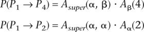
In addition, as the number of populations N increases dramatically, training the transition matrix A(p, p′) becomes challenging because the number of parameters grows quadratically with N. We will address this problem by extending our model to structure the populations hierarchically. For example, suppose we have pairs of similar populations P₁, P₂ (contained in “super-population” P_α) and P₃, P₄ (in P_β). Then, we can decompose the transition matrix A into three matrices A_super, A_α, and A_β as in the following examples:

One modeling assumption intrinsic to HMM-based inference on a sequence is that each locus is only dependent on the previous locus. Although this is approximately correct locally, there are global correlations across the genome that are not captured. For example, if one chromosome contains haploblocks from population p, then the prior probability for p in other chromosomes should be higher. One way to address this might be a multi-pass algorithm that begins with HAPAA inference on the whole genome with uniform priors. Using these estimates of ancestral origin, we update our prior belief of the populations involved, and then rerun inference.

As we continue to gather genomic data for many diverse populations, entirely new directions of research will undoubtedly arise. For example, we will study the shared similarities between populations and begin to characterize their migration patterns. By studying admixture, we may one day be able to reconstruct a detailed map of global human migration and pick out the signals of historical events as well as those not reflected in written records.

References

- Carlson C.S., Eberle M.A., Rieder M.J., Yi Q., Kruglyak L., Nickerson D.A., Eberle M.A., Rieder M.J., Yi Q., Kruglyak L., Nickerson D.A., Rieder M.J., Yi Q., Kruglyak L., Nickerson D.A., Yi Q., Kruglyak L., Nickerson D.A., Kruglyak L., Nickerson D.A., Nickerson D.A. Selecting a maximally informative set of single-nucleotide polymorphisms for association analyses using linkage disequilibrium. Am. J. Hum. Genet. 2004;74:106–120. doi: 10.1086/381000. [DOI] [PMC free article] [PubMed] [Google Scholar]
- Durbin R., Eddy S., Krogh A., Mitchison G., Eddy S., Krogh A., Mitchison G., Krogh A., Mitchison G., Mitchison G. Biological sequence analysis. Cambridge University Press; Cambridge, UK: 1998. [Google Scholar]
- Falush D., Stephens M., Pritchard J., Stephens M., Pritchard J., Pritchard J. Inference of population structure using multilocus genotype data: Linked loci and correlated allele frequencies. Genetics. 2003;164:1567–1587. doi: 10.1093/genetics/164.4.1567. [DOI] [PMC free article] [PubMed] [Google Scholar]
- Halperin E., Eskin E., Eskin E. Haplotype reconstruction from genotype data using imperfect phylogeny. Bioinformatics. 2004;20:1842–1849. doi: 10.1093/bioinformatics/bth149. [DOI] [PubMed] [Google Scholar]
- Hoggart C., Shriver M., Kittles R., Clayton D., McKeigue P., Shriver M., Kittles R., Clayton D., McKeigue P., Kittles R., Clayton D., McKeigue P., Clayton D., McKeigue P., McKeigue P. Design and analysis of admixture mapping studies. Am. J. Hum. Genet. 2004;74:965–978. doi: 10.1086/420855. [DOI] [PMC free article] [PubMed] [Google Scholar]
- International HapMap Consortium A haplotype map of the human genome. Nature. 2005;437:1299–1320. doi: 10.1038/nature04226. [DOI] [PMC free article] [PubMed] [Google Scholar]
- McKeigue P. Mapping genes that underlie ethnic differences in disease risk: Methods for detecting linkage in admixed populations, by conditioning on parental admixture. Am. J. Hum. Genet. 1998;63:241–251. doi: 10.1086/301908. [DOI] [PMC free article] [PubMed] [Google Scholar]
- McVean G.A., Myers S.R., Hunt S., Deloukas P., Bentley D.R., Donnelly P., Myers S.R., Hunt S., Deloukas P., Bentley D.R., Donnelly P., Hunt S., Deloukas P., Bentley D.R., Donnelly P., Deloukas P., Bentley D.R., Donnelly P., Bentley D.R., Donnelly P., Donnelly P. The fine-scale structure of recombination rate variation in the human genome. Science. 2004;304:581–584. doi: 10.1126/science.1092500. [DOI] [PubMed] [Google Scholar]
- Montana G., Pritchard J., Pritchard J. Statistical tests for admixture mapping with case-control and cases-only data. Am. J. Hum. Genet. 2004;75:771–789. doi: 10.1086/425281. [DOI] [PMC free article] [PubMed] [Google Scholar]
- Patterson N., Hattangadi N., Lane B., Lohmueller K., Hafler D., Oksenberg J., Hauser S., Smith M., O’Brien S., Altshuler D., Hattangadi N., Lane B., Lohmueller K., Hafler D., Oksenberg J., Hauser S., Smith M., O’Brien S., Altshuler D., Lane B., Lohmueller K., Hafler D., Oksenberg J., Hauser S., Smith M., O’Brien S., Altshuler D., Lohmueller K., Hafler D., Oksenberg J., Hauser S., Smith M., O’Brien S., Altshuler D., Hafler D., Oksenberg J., Hauser S., Smith M., O’Brien S., Altshuler D., Oksenberg J., Hauser S., Smith M., O’Brien S., Altshuler D., Hauser S., Smith M., O’Brien S., Altshuler D., Smith M., O’Brien S., Altshuler D., O’Brien S., Altshuler D., Altshuler D., et al. Methods for high-density admixture mapping of disease genes. Am. J. Hum. Genet. 2004;74:979–1000. doi: 10.1086/420871. [DOI] [PMC free article] [PubMed] [Google Scholar]
- Redon R., Ishikawa S., Fitch K.R., Feuk L., Perry G.H., Andrews T.D., Fiegler H., Shapero M.H., Carson A.R., Chen W., Ishikawa S., Fitch K.R., Feuk L., Perry G.H., Andrews T.D., Fiegler H., Shapero M.H., Carson A.R., Chen W., Fitch K.R., Feuk L., Perry G.H., Andrews T.D., Fiegler H., Shapero M.H., Carson A.R., Chen W., Feuk L., Perry G.H., Andrews T.D., Fiegler H., Shapero M.H., Carson A.R., Chen W., Perry G.H., Andrews T.D., Fiegler H., Shapero M.H., Carson A.R., Chen W., Andrews T.D., Fiegler H., Shapero M.H., Carson A.R., Chen W., Fiegler H., Shapero M.H., Carson A.R., Chen W., Shapero M.H., Carson A.R., Chen W., Carson A.R., Chen W., Chen W., et al. Global variation in copy number in the human genome. Nature. 2006;444:444–454. doi: 10.1038/nature05329. [DOI] [PMC free article] [PubMed] [Google Scholar]
- Scheet P., Stephens M., Stephens M. A fast and flexible statistical model for large-scale population genotype data: Applications to inferring missing genotypes and haplotypic phase. Am. J. Hum. Genet. 2006;78:629–644. doi: 10.1086/502802. [DOI] [PMC free article] [PubMed] [Google Scholar]
- Stephens M., Smith N.J., Donnelly P., Smith N.J., Donnelly P., Donnelly P. A new statistical method for haplotype reconstruction from population data. Am. J. Hum. Genet. 2001;68:978–989. doi: 10.1086/319501. [DOI] [PMC free article] [PubMed] [Google Scholar]
- Tang H., Coram M., Zhu X., Risch N., Coram M., Zhu X., Risch N., Zhu X., Risch N., Risch N. Reconstructing genetic ancestry blocks in admixed individuals. Am. J. Hum. Genet. 2006;79:1–12. doi: 10.1086/504302. [DOI] [PMC free article] [PubMed] [Google Scholar]
- Tenesa A., Navarro P., Hayes B.J., Duffy D.L., Clarke G.M., Goddard M.E., Visscher P.M., Navarro P., Hayes B.J., Duffy D.L., Clarke G.M., Goddard M.E., Visscher P.M., Hayes B.J., Duffy D.L., Clarke G.M., Goddard M.E., Visscher P.M., Duffy D.L., Clarke G.M., Goddard M.E., Visscher P.M., Clarke G.M., Goddard M.E., Visscher P.M., Goddard M.E., Visscher P.M., Visscher P.M. Recent human effective population size estimate from linkage disequilibrium. Genome Res. 2007;17:520–526. doi: 10.1101/gr.6023607. [DOI] [PMC free article] [PubMed] [Google Scholar]
- Winckler W., Myers S.R., Richter D.J., Onofrio R.C., McDonald G.J., Bontrop R.E., McVean G.A., Gabriel S.B., Reich D., Donnelly P., Myers S.R., Richter D.J., Onofrio R.C., McDonald G.J., Bontrop R.E., McVean G.A., Gabriel S.B., Reich D., Donnelly P., Richter D.J., Onofrio R.C., McDonald G.J., Bontrop R.E., McVean G.A., Gabriel S.B., Reich D., Donnelly P., Onofrio R.C., McDonald G.J., Bontrop R.E., McVean G.A., Gabriel S.B., Reich D., Donnelly P., McDonald G.J., Bontrop R.E., McVean G.A., Gabriel S.B., Reich D., Donnelly P., Bontrop R.E., McVean G.A., Gabriel S.B., Reich D., Donnelly P., McVean G.A., Gabriel S.B., Reich D., Donnelly P., Gabriel S.B., Reich D., Donnelly P., Reich D., Donnelly P., Donnelly P., et al. Comparison of fine-scale recombination rates in humans and chimpanzees. Science. 2005;308:107–111. doi: 10.1126/science.1105322. [DOI] [PubMed] [Google Scholar]
- Zhu X., Cooper R., Elston R., Cooper R., Elston R., Elston R. Linkage analysis of a complex disease through use of admixed populations. Am. J. Hum. Genet. 2004;74:1136–1153. doi: 10.1086/421329. [DOI] [PMC free article] [PubMed] [Google Scholar]
- Zhu X., Luke A., Cooper R., Quertermous T., Hanis C., Mosley T., Gu C., Tang H., Rao D., Risch N., Luke A., Cooper R., Quertermous T., Hanis C., Mosley T., Gu C., Tang H., Rao D., Risch N., Cooper R., Quertermous T., Hanis C., Mosley T., Gu C., Tang H., Rao D., Risch N., Quertermous T., Hanis C., Mosley T., Gu C., Tang H., Rao D., Risch N., Hanis C., Mosley T., Gu C., Tang H., Rao D., Risch N., Mosley T., Gu C., Tang H., Rao D., Risch N., Gu C., Tang H., Rao D., Risch N., Tang H., Rao D., Risch N., Rao D., Risch N., Risch N., et al. Admixture mapping for hypertension loci with genome-scan markers. Nat. Genet. 2005;37:177–181. doi: 10.1038/ng1510. [DOI] [PubMed] [Google Scholar]