

Abstract
We carry out an extensive statistical study of the applicability of normal modes to the prediction of mobile regions in proteins. In particular, we assess the degree to which the observed motions found in a comprehensive data set of 377 nonredundant motions can be modeled by a single normal-mode vibration. We describe each motion in our data set by vectors connecting corresponding atoms in two crystallographically known conformations. We then measure the geometric overlap of these motion vectors with the displacement vectors of the lowest-frequency mode, for one of the conformations. Our study suggests that the lowest mode contains useful information about the parts of a protein that move most (i.e., have the largest amplitudes) and about the direction of this movement. Based on our findings, we developed a Web tool for motion prediction (available from http://molmovdb.org/nma) and apply it here to four representative motions—from bacteriorhodopsin, calmodulin, insulin, and T7 RNA polymerase.
In the analysis of protein dynamics, an important goal is the description of slow large-amplitude motions. These motions, while strongly damped, typically describe conformational changes which are essential for the functioning of proteins. Only global collective motions can significantly change the exposed surface of the protein and hence influence interactions with its environment. Such structural rearrangements in the protein can occur on a local level within a single domain or can involve large movements of protein domains in a multidomain protein. Protein dynamics thus cover a broad timescale: 10−14–10 sec (Wilcox et al. 1988). However, many large-amplitude conformational changes are not on a timescale accessible by most time-dependent theoretical methods, such as phase space sampling techniques (e.g., molecular dynamics). Therefore, in order to gain insight into the mechanism of slow, large-amplitude motions, one must resort to the use of a time-independent approach, such as normal mode analysis (Levitt et al. 1985).
Normal mode analysis (NMA) is a fast and simple method to calculate vibrational modes and protein flexibility. In NMA, sometimes restrained to Cα atoms only, the atoms are modeled as point masses connected by springs, which represent the interatomic force fields. One particular type of NMA is the elastic network model. In this model, the springs connecting each node to all other neighboring nodes are of equal strength, and only the atom pairs within a cutoff distance are considered.
All existing NMA techniques have important common limitations resulting from the use of the harmonic approximation, the neglect of solvent damping, and the absence of information about energy barriers and multiple minima on the potential energy surface (Elber and Karplus 1987; Frauenfelder et al. 1988; Hong et al. 1990). In fact, the most interesting biologically significant low-frequency motions in a realistic environment are overdamped and hence not vibrational at all, rendering the corresponding normal mode frequencies of little physical significance (Go et al. 1983; Kottalam and Case 1990; Horiuchi and Go 1991; Amadei et al. 1993). Therefore, the identification and characterization of low-frequency domain motions by using NMA might seem questionable. Nevertheless, comparisons of low-frequency normal modes and the directions of large-amplitude fluctuations in molecular dynamics simulations indicate clear similarities (Amadei et al. 1993; Hayward et al. 1997). Close directional coincidence of the lowest normal mode axes and the first principal component axes obtained from molecular dynamic simulations has been observed (Hayward et al. 1997). In addition, the axes of the first modes were found to be overwhelmingly closure axes. A lesser degree of correspondence was observed for the second modes.
It has also been shown that the low-frequency modes describing the large-scale real-world motions of a protein can be related to fundamental biological characteristics (Brooks and Karplus 1985; Thomas et al. 1999). For example, Bahar and Jernigan (1998) successfully analyzed the vibrational dynamics of transfer RNAs, both free and complexed with the cognate synthetase, using the elastic network model. They examined the global mode of motion of tRNAGln complexed with glutaminyl-tRNA synthetase, and established that certain residues that cluster near the ATP binding site form a hinge-bending region controlling the cooperative motion and thereby the catalytic function of the enzyme. Normal modes have been successfully used to display concerted motions of proteins (Noguti and Go 1982; Brooks and Karplus 1983; Go et al. 1983; Levy et al. 1984; Levitt et al. 1985; Henry et al. 1986), including slow motions between protein domains as in the hinge-bending motion of lysozyme (Brooks and Karplus 1985; Gibrat and Go 1990). It was recently shown that the first step of the gating mechanism in the mechanosensitive channel (MscL) can be described with only the three lowest-frequency modes (Valadie et al. 2003). Those results clearly indicate that the movement associated with these modes is an iris-like movement involving both tilts and twists. Several other works showed that low-frequency modes overlap with real conformational changes (Thomas et al. 1999; Tama and Sanejouand 2001). There is also evidence to suggest that proper, symmetric normal mode vibration of binding pockets is crucial to correct biological activity in some proteins (Thomas et al. 1996a,b; Hinsen 1998).
Experimental data on protein motions from incoherent neutron scattering and resulting observations of the density of states were also found to agree with simulations (Smith et al. 1987; Cusack et al. 1988). In particular, inelastic neutron scattering spectra have resolved the density of states for myoglobin in the low-frequency regime at room temperature (Cusack and Doster 1990). Site-selective fluorescence spectroscopy of Zn-substituted myoglobin has obtained this density without the use of model shape functions (Ahn et al. 1993). Resonance Raman spectra generated by psec laser pulses have also been interpreted by analyzing relaxation of protein normal modes (Alden et al. 1992).
Despite the large body of successful NMA applications in protein dynamics studies, both theoretical and experimental normal modes have only been compared to actual motions on a case-by-case basis. Few analyses have attempted to do this comprehensively in a database framework. Thus, the need for statistical assessment of the overall reliability and applicability of NMA to the description of various aspects of protein motion becomes apparent. In our previous work (Krebs et al. 2002) we performed a large-scale database study of molecular motions within the MolMovDB (Gerstein and Krebs 1998; Krebs and Gerstein 2000; Echols et al. 2003) framework. The results indicate that the lowest-frequency normal mode contributes the most to the decomposition of the real (observed) motion in a linear combination of the first 20 normal modes, in agreement with the findings mentioned above. In the present work, we asked to what degree the direction of the observed motion, described by vectors connecting corresponding atoms of a protein in its initial and final conformation, coincides with the displacement vectors of the lowest normal modes for the initial conformation. Since structure pairs may not always be available, the other main motivation behind this work was to develop an easy-to-use motion prediction technique capable of assessing the direction of the actual protein motion.
Therefore, we constructed a comprehensive set of observed nonredundant molecular motions which we used to assess the quality of NMA predictions. If structures of two alternative conformations (one assigned to be “initial” and the other, “final”) are known, a direct comparison can be done between the difference vector of the two conformations and the calculated displacement vector of the lowest normal mode. Our results suggest that the top 2%–3% of the most significant interdomain movements in a protein can nevertheless be modeled successfully by a set of the corresponding lowest normal mode displacement vectors. We developed ab initio selection criteria based on either indirect experimental evidence (B-factors) or structural variability within the corresponding fold family (in the multiple structural alignment sense) to single out those NMA displacement vectors that accurately model the most mobile parts of the molecule. Since portions of the molecule moving the most usually represent the most “biologically interesting” parts in a protein and normally serve as an approximate description of the overall motion, the goal of obtaining a fast qualitative prediction of the overall motion has been achieved.
Results and Discussion
Constructing a new set of nonredundant motions
The set of all chain sequences (~33,000 entries) extracted from all crystallographically determined proteins deposited in the PDB was subjected to all-versus-all sequence alignment using the FASTA program (Pearson and Lipman 1988). The pairs with greater than 99% identity (~700,000 pairs) were selected for the initial pool of tentative motions. Structural alignment for this set of tentative structure pairs was performed using the Least Square Fit (LSQ) method to select pairs with root-mean-squared deviation (RMSD) greater than 1.5 Å. To achieve an optimal superposition of the two structures, we used our in-house structural alignment routine, which finds the solution for the parameters of the RMSD-minimizing rotation matrix (RM) as suggested by Kabsch (1976). This RMSD value was used to select the final (comprehensive) set of structures within the chosen RMSD cutoff of 1.5 Å.
In this comprehensive set of 13,571 structure pairs, 11,217 were successfully “morphed,” i.e., a motion pathway could be constructed by the morph server. From those, 7467 were located in the CATH database (Orengo et al. 1997) by their PDB and chain identifiers (Fig. 2 ▶). Morphs falling into the same near-identical CATH level (defined as all sequences with 99% identity) were taken and examined collectively to identify a single best representative morph. Where possible, structure pairs with one domain missing were discarded and the groupings were further reduced by taking only those pairs with sequence length greater than the mean for each set, thus eliminating truncated proteins. Finally, the morph with the median overall RMSD between the initial and final frames was selected as the representative entry. In those families where the set was too small to perform this procedure, the morph with the highest RMSD (and in some cases, the only available morph) was selected by default. Thus the final (nonredundant) set of 377 morphs had no more than 95% sequence identity between any two entries. These morphs, in the context of the overall CATH schema, are displayed at http://molmovdb.org/nma.
Figure 2.

An illustration of the scheme that was used to identify the data set of nonredundant domain motions.
We calculated a histogram of RMSD values for our new nonredundant set of motion pairs (Fig. 3 ▶). It shows that more than 90% of the RMSD values lie in the 1.5–5.5 Å interval.
Figure 3.

Distribution of RMSD scores (in Å) for the nonredundant set of domain motions.
Statistical analysis of NMA directional correlations with observed motions
We used an average correlation cosine squared, which we further refer to as the S-statistic (equation 4), as an overall quantitative measure of the NMA predicted motions. This quantity simply reflects the degree of average directional similarity between the observed motion vectors and the normal mode displacement vectors. The larger values of S correspond to the lower average angle between the two sets of vectors.
First, we calculated the value of S and S2 for each motion pair in our data set, and plotted histograms of these values (Figs. 4 ▶, 5 ▶). The S2 statistic appears to be useful because the corresponding values of the average angle are mapped more uniformly to the interval [0..1]. To get a rough estimate of the average value for the directional overlap, one assumes that all atoms in a structure pair have a similar overlap Õi Then the peak (most common) value 0.48 of S2 in the histogram would imply (see equation 4) an average angle θ̃i of 51°, the angle between a typical normal mode displacement vector and an actual motion vector for the same Cα. This average value of θ̃i only marginally differs from the value of 54.7° (Arfken and Weber 2000) between a pair of randomly generated 3D vectors.
Figure 4.

Histogram of S2 statistic and the corresponding average θj angle. Values are shown for 100% (dotted), 10% (dashed), and 2.5% (solid) of selected Cα-atoms based on the motion amplitudes in the nonredundant data set of domain motions. Selection of the most moving atoms results in larger values of S2 (the larger values of S and S2 correspond to the lower average angle between the two sets of vectors). Dotted line points to the location of equal to 54.7°, the average angle between two randomly θj generated vectors.
Figure 5.

S-statistic as a function of percentage of the largest selected Cα displacements for single-domain and multidomain protein motions.
The behavior of the S-statistic was also studied as a function of the percentage of the selected Cαs. Cαs were selected based upon the length of the vector representing the actual movement of that particular Cα. S-statistics were calculated again for the selected atoms. The histograms for the S50% and S2.5% (S values calculated for the 10% and 2.5% of the most moving Cαs, respectively) are shown in Figure 4 ▶. The average value of both S50% and S2.5% shifts to the right (S2.5% has no real peak anymore). The same trend (higher values of S for fewer selected atoms) can be seen in Figure 5 ▶, where S is plotted as a function of the percent of selected atoms. These results suggest that the direction of motion is predicted most accurately for Cα atoms that move the most.
Conveniently, these are the atoms we are most interested in because just a few such atoms are needed to give an idea what the overall protein motion looks like. We propose that NMA (or at least the lowest-frequency mode) is not suitable for providing accurate details for all of the constituent atoms in a biological system, but has a selective accuracy in capturing the large, concerted motion features of a given macromolecule.
Representative examples of correlations with observed motions
Here we describe several examples we have chosen from our comprehensive set, typical representatives of different major classes of motions, to illustrate our approach. In particular, we picked a small fragment shear motion (insulin), a small domain shear motion (bacteriorhodopsin), domain hinge motion (calmodulin), and a large-scale multidomain refolding motion (T7 polymerase), for which both initial and final conformations are experimentally available (Yin and Steitz 2002). S-values for these motions are plotted in Figure 5 ▶. One can see that except for T7, the S values for all the individual structures exhibit consistent performance as the overall 377 single-domain set with regard to selection. Predicted directions of motion for the four most mobile Cαs are shown in Figure 6, A–D ▶. In all cases, the predicted largest movement and the observed one superpose well. They involve the same atoms and point in “similar” directions. These predictions appear to be very helpful in deducing plausible mechanisms of protein function.
Figure 6.

Real motion (red) and NMA-predicted (blue) vectors for the motion of (A) insulin (d7insb_SCOP domain), (B) calmodulin (d2bbm_domain), (C) bacteriorhodopsin (d1c8sa_SCOP domain), and (D) T7 polymerase (elongation complex). In D, labels 1, 2 , 3, and 4 represent residues THR 596, VAL 597, THR 598, and GLY 603, respectively. Arrows indicate only the directions of the motion.
1. Insulin
In Figure 6A ▶ we show the predicted motions of insulin. The first and foremost conclusion of structural studies of insulin is that the protein is extremely flexible and adaptable. Numerous crystal forms depending on their specific T and R conformations are known (Chothia et al. 1983; Hua et al. 1991; Hawkins et al. 1994, 1995; Ye et al. 1996, 2001; Bao et al. 1997; Whittingham et al. 1997; Schlein et al. 2000; Dupradeau et al. 2002). The flexibility is especially marked in the B chain: The conformation of the N terminus gives rise to the T and R naming system, and the flexibility of the C terminus is thought to be very important in a conformational change necessary for receptor binding. In Figure 6A ▶, the vectors representing our predicted motion of insulin suggest that chain B is indeed quite mobile: All significant motion vectors are located in chain B. Furthermore, the vector of motion at residue PHE 1B pointing along the helix axes suggests that this whole helix participates in a concerted motion. The other three vectors in the hinge region (PRO 28B, LYS 29B, and ALA 30B) pointing in almost perpendicular direction to the first vector, suggest that the motion of chain B is a small fragment shear motion. This result relates to the experimental evidence that the β-turn motion in chain B (residues B24–B30) is essential for the enzymatic activity of insulin (Bao et al. 1997).
2. Calmodulin
Figure 6B ▶ shows the predicted movement of calmodulin, a ubiquitous eukaryotic Ca2+-binding protein that participates in numerous cellular regulatory processes. The X-ray structure (Babu et al. 1985, 1987, 1988; Kretsinger et al. 1986) of this highly conserved 148-residue protein has a dumbbell-like shape in which two globular domains are connected by a seven-turn α-helix. The binding of Ca2+ to either domain induces a conformational change in that domain, which further induces some other catalytic activity (such as activation of phosphorylase kinase). Much effort was put into determining the details of calmodulin structure and the mechanism of its Ca2+-induced conformational change (Kretsinger et al. 1986; Sekharudu and Sundaralingam 1993; Cook et al. 1994; Chin et al. 1997; Wilson and Brunger 2000; Kurokawa et al. 2001; Han et al. 2002; Hoelz et al. 2003; Yamauchi et al. 2003). The results of our calculations help to interpret the available experimental data. The vectors of the predicted largest moving parts of the molecule (Fig. 6B ▶) indicate the direction along which the EF-hand is most likely to move. This movement, in agreement with the existing experimental evidence (Persechini and Kretsinger 1988; Reuland et al. 2003) also suggests that calmodulin’s central helix serves as a flexible rather than as a rigid spacer, a property that probably further increases the range of target sequences to which calmodulin can bind (Putkey et al. 1988).
3. Bacteriorhodopsin
Bacteriorhodopsin undergoes conformational changes during its catalytic cycle. These conformational changes are mainly restricted to the cytoplasmic side of the protein and for the most part involve helices E, F, and G. This conformational change represents a crucial step in the activity of the native protein (Luecke et al. 1999; Subramaniam et al. 1999; Sass et al. 2000). The largest predicted motions in bacteriorhodopsin are shown in Figure 6C ▶. We observe the largest movements for residues VAL101 (helix C), PHE153 (helix E), and VAL177 (helix F) on the cytoplasmic side of the protein. Our prediction of the described movements of the cytoplasmic ends of the helices correlates well with the experimentally observed structural changes related to the functional activity of bacteriorhodopsin (Luecke et al. 1999; Subramaniam et al. 1999; Luecke 2000).
4. T7 Polymerase
Studies of the bacteriophage T7 RNA polymerase reaction are crucial in the fundamental understanding of the mechanism of transcription (Jia and Patel 1997a,b), and are also important in biotechnology development (Roe et al. 1988; Majumdar et al. 1989). The high efficiency of T7 RNAP makes it a widely used tool in producing RNA in vitro and in microarray gene expression. The motion of T7 RNA polymerase is one of the largest recorded motions in the MolMovDB by any set of criteria. It involves partial refolding of about 250 residues in the N-terminal domain in order to unbind the promoter and open up an exit channel for the nascent RNA (Yin and Steitz 2002). Conformational changes this large are not unheard of (e.g., fusion-triggering conformational change of a fusion domain from influenza hemagglutinin) (Bullough et al. 1994; Han et al. 2001). Still, a motion of this size is quite unexpected for a polymerase that is in the act of transcribing RNA. There is a good chance that additional intermediate stages exist (Y. Yin and T. Steitz, pers. comm.). The normal mode characteristics of the motion for this large multidomain protein differ significantly from the single-domain motions both in terms of the magnitudes of the displacement vectors and statistical characteristics. For the three single-domain proteins mentioned above, the S-statistic exhibits the same behavior as the one calculated for the whole data set, i.e., S reaches its maximal values (minimal average θ̃i) for those atoms that move the most. It turns out that a restricted Cα selection based on anticipated motion magnitude is not necessary for T7 polymerase. Moreover, for T7 polymerase, NMA predicts the direction of movement for all Cαs with slightly greater accuracy compared to the predictions for 2.5% the Cαs with the largest motions in our single-domain motion set. This probably happens because the employed NMA allows one to see only the most prominent details of motion, which are better distinguished in a concerted multidomain movement than in a smaller fragment motion. Recently Cui et al. (2004) determined that “the character of the lowest-frequency modes of the β(E) subunit is highly correlated with the large β(E) to β(TP) transition,” which is in agreement with our findings. However, more experimental data are needed to prove whether NMA is better suited for larger motions.
Selection criteria for single-structure predictions
The above analysis suggests that the information about the protein motion contained in the lowest-frequency normal mode vectors can be divided into two parts: (1) the part related to the large-amplitude concerted motion and (2) the smaller scale part related to local “jittering.” We can exclude the latter part if we restrict our attention to the atoms that move the most.
It becomes apparent that additional criteria are necessary to ensure a reliable prediction of the largest motions when only one conformation is available. The ability to predict atoms that move the most as well as the directions of their motion can be very useful for gaining further insight about the mechanism of protein function in cases where conformational changes are unknown or where no high-resolution structures exist.
In general, Cαs with large motions cannot be reliably selected based on the calculated NMA amplitudes—the correlation coefficient between the sets of normal mode displacements and the corresponding real motion vectors in our data set turns out to be only 0.34. Therefore, we used B-factors to select the Cαs with the largest motion vectors. The correlation coefficient calculated for the B-factors versus observed motion amplitudes averaged over our data set appeared to be 0.77. When predicting the direction of the motion, we are guaranteed on average to have seven or eight out of 10 atoms that move the most in our NMA description of the real motion based on a B-factor selection criterion. When B-factors for a particular structure are not available, one can select the Cαs that move the most based on their structural variation in the multiple structural alignment for the corresponding fold family. In our study, we built multiple structural alignments for every motion pair in our data set in the following way: For each initial conformation, 10 structures (if available) were selected from the corresponding fold family. In order to find an average core structure, the 10 structures are aligned and the average RMSD value is minimized (Alexandrov and Gerstein 2004). The Cα consensus positions with the largest structural deviation are assumed to represent the positions that move the most in the observed motion of the original structure. The correlation coefficient between the positional variations and the observed motion amplitudes averaged among all Cαs in the data set was found to be 0.83. Thus, the core structures can serve as an independent reliable criterion for selecting the most mobile atoms in a protein family and particularly for NMA predictions of directions of motions.
Results of single structure predictions from testing and training data
Since the number of proteins in our nonredundant set of motions is limited, we refined the cut-off value for our S-statistic by using 10-fold cross-validation. The data set of 377 proteins was split into 10 equally balanced subsets, each containing ~38 structures from the original set. Structures in each subset were selected completely randomly. Each structure belonged to only a single subset, and there were no duplicated structures in any subset. The optimal value for the cutoff, which turned out to be 2.5%, has been determined in each subset based on the remaining ~340 structures that belonged to the other nine subsets.
In practice, selecting four atoms based on their B-factors for a single structure is sufficient to satisfy this threshold requirement, as well as to build an overall qualitative picture of the overall protein motion. Motion prediction based on only a single “best” atom selection is also a viable alternative. The distribution of average absolute angles
 |
based on the one-atom θ̃1(B)and four-atom θ̃4(B) largest B-factor selection criteria for the entire data set is shown in Figure 7 ▶. Both distributions appear to be very similar. One can see that accurate motion direction predictions (<30° deviation from the observed direction) occur commonly but not all the time. This is expected, however since NMA is not a very accurate description of real-life motion and the longest trajectory in a protein motion is rarely a straight line. Therefore, an otherwise correctly predicted initial direction of motion (NMA prediction) might deviate noticeably from the vector connecting its initial and final positions. This suggests, in turn, that a picture represented by four atoms with the largest B-factors tends to be a better visual description of the overall motion, particularly in cases involving hinge motion or large-domain motion (from a statistical point of view, however, both one-atom and four-atom motion descriptions are nearly equivalent, since they both satisfy the 2.5% selection criterion).
Figure 7.

Histogram of the average angle between the lowest-frequency normal mode vectors and the corresponding observed displacement vectors for the selected Cα with the largest B-factors in the nonredundant data set of domain motions. θ4(B) distribution is represented by the solid line, and θ1(B) by the dashed line.
Implementation of working prediction server
We have set up an NMA Web tool at http://molmovdb.org//nma/ to illustrate the main findings in the paper and to provide a motion-prediction service to the community (Fig. 8 ▶). The tool allows a researcher to identify the key residues involved in the motion and their most probable direction. Given either a PDB/SCOP ID or an uploaded structure (Fig. 8A ▶), the server calculates the lowest normal mode of the submitted query, finds and highlights the most mobile structural regions, and shows the direction of the four Cα atoms that move the most (Fig. 8B ▶). Selection of the four most accurate NMA vectors is based on either supplied B-factors or the prebuilt multiple structural alignment for the corresponding fold family. The four selected atoms are shown in red in the calculated lowest-frequency-normal-mode movie. A static picture with all residues ranked and highlighted based on their motion amplitudes (red, largest motion; blue, smallest motion) is also provided (Fig. 8B ▶).
Figure 8.

Screenshot of the NMA motion and flexibility prediction server: (A) input page and (B) results page.
Conclusion
An extensive statistical study to show the applicability of Normal Mode Analysis to the prediction of protein flexibility was performed on a new, comprehensive data set of nonredundant single-domain motions. The motions were modeled by using the lowest-frequency normal mode, and predictions were assessed by directional overlap statistics. Our results suggest that it is possible to extract information from the lowest-frequency normal mode, which identifies the most mobile parts of the protein as well as their directions by focusing on a few Cα atoms that move the most. We propose that the lowest-frequency NMA can selectively predict the atoms and the direction of conformational changes occurring in proteins. While the normal mode analysis is based on finding vibrations that do not actually occur in the over-damped condition of a protein in its environment, it appears to usefully indicate the propensity of the structure to change in a particular direction. We find that motion prediction gains reliability if additional criteria, such as crystallographic B-factors and RMSD values from multiple structural alignments, are built into the motion analysis. A Web tool for prediction of protein motion and flexibility was developed to demonstrate the described approach.
Materials and methods
Basic NMA framework and its MMTK implementation
See Figure 1 ▶ for the notation used throughout. The concept of Normal Mode Analysis is to find a set of basis vectors (normal modes) describing the molecule’s concerted atomic motion and spanning the set of all 3N - 6 degrees of freedom. For very large molecules, it is often of more interest to find a small subset of these normal modes that in some way seem especially important. By modeling the interatomic bonds as springs and analyzing the protein as a large set of coupled harmonic oscillators, one can calculate a frequency of periodic motion associated with each normal mode, and then attempt to find normal modes with low frequencies.
Figure 1.
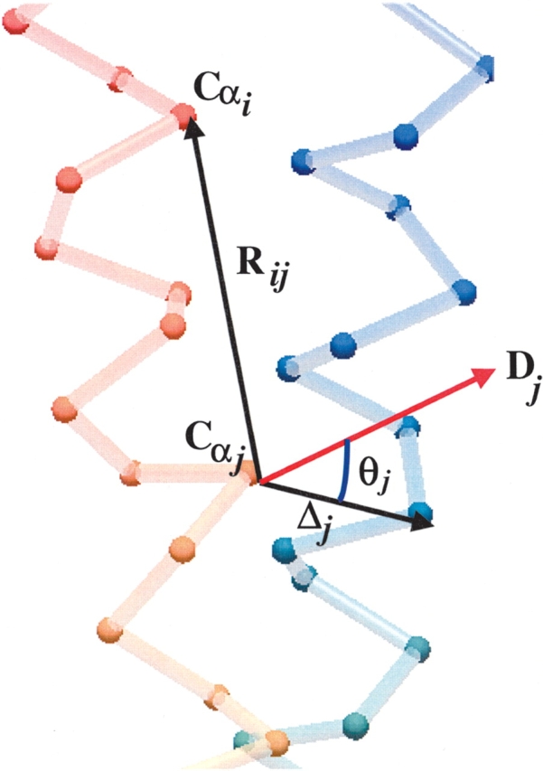
Notations used in the paper. Rij is the vector connecting atom i to atom j in the experimental (initial) structure. Δj is the difference vector between atom i in the displaced (final) structure and the same atom in the initial structure. Dj is the lowest normal mode displacement vector for atom j in the initial conformation. θj is the angle between vectors Dj and Δj for atom j.
The principal of normal mode analysis is to solve an eigenvalue equation of the form
 |
(1) |
where q is a vector representing the displacements in three dimensions of the various atoms of the molecule, and F is a matrix that can be computed from the mass of the system and potential energy functions. Solutions to the above system are vectors of periodic functions (the normal modes) vibrating in unison at the characteristic frequency of the mode.
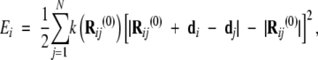
We used MMTK (Hinsen 2000) to carry out NMA on preprocessed PDB file pairs containing only Cα coordinates. The numerical Python module (Ascher et al. 2000) was employed to carry out all linear algebra computations. Each residue was approximated as a single virtual atom with mass of the corresponding amino acid and centered at its Cα coordinate. The MMTK deformation force field was used to model interatomic Cα interactions. In this model, the energy is computed as the difference between a displaced model and the experimental structure using the formula:
 |
(2) |
where k is a constant, Rij(0) is the vector connecting atom i to atom j in the experimental structure, di is the difference vector between atom i in the displaced (final) structure and the same atom in the initial structure. Furthermore, in the practical implementation of the NMA used here (Hinsen 2000), the force constant value decreases with distance as an exponential function to allow its efficient evaluation with a cutoff not significantly larger then the interatomic equilibrium distance R(0)ij.
In order to accelerate our computations, we restricted MMTK to compute only the 20 lowest-frequency normal modes. In our earlier work (Krebs et al. 2002) we showed that this truncation is adequate for qualitative characterization of the lowest-frequency protein motions.
Statistical measures for assessing overlap
A means of quantifying the similarity of the displacement between the PDB structures and the normal mode displacement vectors can be achieved in terms of the following quantities:
 |
(3) |
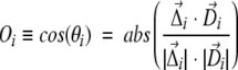
In the above formula, we define the “directional overlap” Oi for one particular atom i as the absolute value of the cosine of the angle between the displacement vector D→i of the lowest frequency mode and the observed direction of motion Δ→i (Fig. 1 ▶).
We use these individual directional overlaps to define the Oi second order statistic, S-statistic:
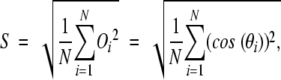 |
(4) |
which serves as an overall quantitative measure of the similarity in directionality between the observed motion vectors and the normal mode displacement vectors.
We also define an overlap measure in relation to atom selection. The quantity SP% is defined as
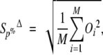 |
(5) |
where the sum is carried over the first P percent of Cαs with the largest difference vectors Δ→i (M ≡ N • 0.01P). When the number of selected atoms is small, it is convenient to rewrite the quantity SΔP% as
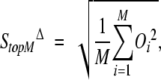 |
(6) |
in order to explicitly indicate the number M of Cαs with the largest difference vectors entering the sum in equations 5 and 6. Quantities SBP% and SBtopM are defined in exactly the same way as their counterparts SΔP% and SΔtopM except that the selection of Cαs is carried with respect to their corresponding B-factors, rather than the difference vectors.
For robustness, we can also define an average angle θ̃ (B)N
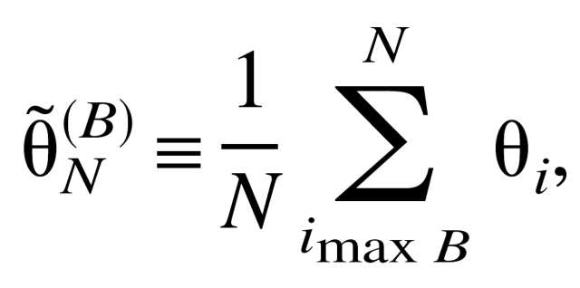 |
(7) |
where summation is carried over N < M angles θ̃i corresponding to the Cα atoms with the largest B-factors.
Acknowledgments
M.G. thanks the NIH (grant P01 GM54160) for support. U.L. thanks the DAAD for a postdoctoral fellowship.
Article and publication are at http://www.proteinscience.org/cgi/doi/10.1110/ps.04882105.
References
- Ahn, J.S., Kanematsu, Y., and Kushida, T. 1993. Site-selective fluorescence spectroscopy in dye-doped polymers. I. Determination of the site-energy distribution and the single-site fluorescence spectrum. Phys. Rev. B Condens. Matter 48 9058–9065. [DOI] [PubMed] [Google Scholar]
- Alden, R., Schneebeck, M., Ondrias, M., Courtney, S., and Friedman, J. 1992. Mode-specific relaxation dynamics of photoexcited Fe(II) protoporphyrin IX in hemoglobin. J. Raman Spectrosc. 23 569–574. [Google Scholar]
- Alexandrov, V. and Gerstein, M. 2004. Using 3D hidden Markov models that explicitly represent spatial coordinates to model and compare protein structures. BMC Bioinformatics 5 2. [DOI] [PMC free article] [PubMed] [Google Scholar]
- Amadei, A., Linssen, A.B., and Berendsen, H.J. 1993. Essential dynamics of proteins. Proteins 17 412–425. [DOI] [PubMed] [Google Scholar]
- Arfken, G.B. and Weber, H. 2000. Mathematical methods for physicists. Academic Press, New York.
- Ascher, D., Dubois, P.F., Hinsen, K., Hugunin, J., and Oliphant, T. 2000. Numerical python. Lawrence Livermore National Laboratory, Livermore, CA.
- Babu, Y.S., Sack, J.S., Greenhough, T.J., Bugg, C.E., Means, A.R., and Cook, W.J. 1985. Three-dimensional structure of calmodulin. Nature 315 37–40. [DOI] [PubMed] [Google Scholar]
- Babu, Y.S., Bugg, C.E., and Cook, W.J. 1987. X-ray diffraction studies of calmodulin. Methods Enzymol. 139 632–642. [DOI] [PubMed] [Google Scholar]
- ———. 1988. Structure of calmodulin refined at 2.2 Å resolution. J. Mol. Biol. 204 191–204. [DOI] [PubMed] [Google Scholar]
- Bahar, I. and Jernigan, R.L. 1998. Vibrational dynamics of transfer RNAs: Comparison of the free and synthetase-bound forms. J. Mol. Biol. 281 871–884. [DOI] [PubMed] [Google Scholar]
- Bao, S.J., Xie, D.L., Zhang, J.P., Chang, W.R., and Liang, D.C. 1997. Crystal structure of desheptapeptide(B24–B30)insulin at 1.6 Å resolution: Implications for receptor binding. Proc. Natl. Acad. Sci. 94 2975–2980. [DOI] [PMC free article] [PubMed] [Google Scholar]
- Brooks, B. and Karplus, M. 1983. Harmonic dynamics of proteins: Normal modes and fluctuations in bovine pancreatic trypsin inhibitor. Proc. Natl. Acad. Sci. 80 6571–6575. [DOI] [PMC free article] [PubMed] [Google Scholar]
- ———. 1985. Normal modes for specific motions of macromolecules: Application to the hinge-bending mode of lysozyme. Proc. Natl. Acad. Sci. 82 4995–4999. [DOI] [PMC free article] [PubMed] [Google Scholar]
- Bullough, P.A., Hughson, F.M., Skehel, J.J., and Wiley, D.C. 1994. Structure of influenza haemagglutinin at the pH of membrane fusion. Nature 371 37–43. [DOI] [PubMed] [Google Scholar]
- Chin, D., Winkler, K.E., and Means, A.R. 1997. Characterization of substrate phosphorylation and use of calmodulin mutants to address implications from the enzyme crystal structure of calmodulin-dependent protein kinase I. J. Biol. Chem. 272 31235–31240. [DOI] [PubMed] [Google Scholar]
- Chothia, C., Lesk, A.M., Dodson, G.G., and Hodgkin, D.C. 1983. Transmission of conformational change in insulin. Nature 302 500–505. [DOI] [PubMed] [Google Scholar]
- Cook, W.J., Walter, L.J., and Walter, M.R. 1994. Drug binding by calmodulin: Crystal structure of a calmodulin-trifluoperazine complex. Biochemistry 33 15259–15265. [DOI] [PubMed] [Google Scholar]
- Cui, Q., Li, G., Ma, J., and Karplus, M. 2004. A normal mode analysis of structural plasticity in the biomolecular motor F(1)-ATPase. J. Mol. Biol. 340 345–372. [DOI] [PubMed] [Google Scholar]
- Cusack, S. and Doster, W. 1990. Temperature dependence of the low frequency dynamics of myoglobin. Measurement of the vibrational frequency distribution by inelastic neutron scattering. Biophys. J. 58 243–251. [DOI] [PMC free article] [PubMed] [Google Scholar]
- Cusack, S., Smith, J., Finney, J., Tidor, B., and Karplus, M. 1988. Inelastic neutron scattering analysis of picosecond internal protein dynamics. Comparison of harmonic theory with experiment. J. Mol. Biol. 202 903–908. [DOI] [PubMed] [Google Scholar]
- Dupradeau, F.Y., Richard, T., Le Flem, G., Oulyadi, H., Prigent, Y., and Monti, J.P. 2002. A new B-chain mutant of insulin: Comparison with the insulin crystal structure and role of sulfonate groups in the B-chain structure. J. Pept. Res. 60 56–64. [DOI] [PubMed] [Google Scholar]
- Echols, N., Milburn, D., and Gerstein, M. 2003. MolMovDB: Analysis and visualization of conformational change and structural flexibility. Nucleic Acids Res. 31 478–482. [DOI] [PMC free article] [PubMed] [Google Scholar]
- Elber, R. and Karplus, M. 1987. Multiple conformational states of proteins: A molecular dynamics analysis of myoglobin. Science 235 318–321. [DOI] [PubMed] [Google Scholar]
- Frauenfelder, H., Parak, F., and Young, R.D. 1988. Conformational substates in proteins. Annu. Rev. Biophys. Biophys. Chem. 17 451–479. [DOI] [PubMed] [Google Scholar]
- Gerstein, M. and Krebs, W. 1998. A database of macromolecular motions. Nucleic Acids Res. 26 4280–4290. [DOI] [PMC free article] [PubMed] [Google Scholar]
- Gibrat, J.F. and Go, N. 1990. Normal mode analysis of human lysozyme: Study of the relative motion of the two domains and characterization of the harmonic motion. Proteins 8 258–279. [DOI] [PubMed] [Google Scholar]
- Go, N., Noguti, T., and Nishikawa, T. 1983. Dynamics of a small globular protein in terms of low-frequency vibrational modes. Proc. Natl. Acad. Sci. 80 3696–3700. [DOI] [PMC free article] [PubMed] [Google Scholar]
- Han, X., Bushweller, J.H., Cafiso, D.S., and Tamm, L.K. 2001. Membrane structure and fusion-triggering conformational change of the fusion domain from influenza hemagglutinin. Nat. Struct. Biol. 8 715–720. [DOI] [PubMed] [Google Scholar]
- Han, B.G., Han, M., Sui, H., Yaswen, P., Walian, P.J., and Jap, B.K. 2002. Crystal structure of human calmodulin-like protein: Insights into its functional role. FEBS Lett. 521 24–30. [DOI] [PubMed] [Google Scholar]
- Hawkins, B.L., Cross, K.J., and Craik, D.J. 1994. A 1H-NMR determination of the solution structure of the A-chain of insulin: Comparison with the crystal structure and an examination of the role of solvent. Biochim. Biophys. Acta 1209 177–182. [DOI] [PubMed] [Google Scholar]
- Hawkins, B., Cross, K., and Craik, D. 1995. Solution structure of the B-chain of insulin as determined by 1H NMR spectroscopy. Comparison with the crystal structure of the insulin hexamer and with the solution structure of the insulin monomer. Int. J. Pept. Protein Res. 46 424–433. [DOI] [PubMed] [Google Scholar]
- Hayward, S., Kitao, A., and Berendsen, H.J. 1997. Model-free methods of analyzing domain motions in proteins from simulation: A comparison of normal mode analysis and molecular dynamics simulation of lysozyme. Proteins 27 425–437. [DOI] [PubMed] [Google Scholar]
- Henry, E.R., Eaton, W.A., and Hochstrasser, R.M. 1986. Molecular dynamics simulations of cooling in laser-excited heme proteins. Proc. Natl. Acad. Sci. 83 8982–8986. [DOI] [PMC free article] [PubMed] [Google Scholar]
- Hinsen, K. 1998. Analysis of domain motions by approximate normal mode calculations. Proteins 33 417–429. [DOI] [PubMed] [Google Scholar]
- ———. 2000. The molecular modeling toolkit: A new approach to molecular simulations. J. Comp. Chem. 21 79–85. [Google Scholar]
- Hoelz, A., Nairn, A.C., and Kuriyan, J. 2003. Crystal structure of a tetradeca-meric assembly of the association domain of Ca2+/calmodulin-dependent kinase II. Mol. Cell 11 1241–1251. [DOI] [PubMed] [Google Scholar]
- Hong, M.K., Braunstein, D., Cowen, B.R., Frauenfelder, H., Iben, I.E., Mourant, J.R., Ormos, P., Scholl, R., Schulte, A., Steinbach, P.J., et al. 1990. Conformational substates and motions in myoglobin. External influences on structure and dynamics. Biophys. J. 58 429–436. [DOI] [PMC free article] [PubMed] [Google Scholar]
- Horiuchi, T., and Go, N. 1991. Projection of Monte Carlo and molecular dynamics trajectories onto the normal mode axes: Human lysozyme. Proteins 10 106–116. [DOI] [PubMed] [Google Scholar]
- Hua, Q.X., Shoelson, S.E., Kochoyan, M., and Weiss, M.A. 1991. Receptor binding redefined by a structural switch in a mutant human insulin. Nature 354 238–241. [DOI] [PubMed] [Google Scholar]
- Jia, Y. and Patel, S.S. 1997a. Kinetic mechanism of GTP binding and RNA synthesis during transcription initiation by bacteriophage T7 RNA polymer-ase. J. Biol. Chem. 272 30147–30153. [DOI] [PubMed] [Google Scholar]
- ———. 1997b. Kinetic mechanism of transcription initiation by bacteriophage T7 RNA polymerase. Biochemistry 36 4223–4232. [DOI] [PubMed] [Google Scholar]
- Kabsch, W. 1976. A solution for the best rotation to relate two sets of vectors. Acta Cryst. A32 922–923. [Google Scholar]
- Kottalam, J. and Case, D.A. 1990. Langevin modes of macromolecules: Applications to crambin and DNA hexamers. Biopolymers 29 1409–1421. [DOI] [PubMed] [Google Scholar]
- Krebs, W.G. and Gerstein, M. 2000. The morph server: A standardized system for analyzing and visualizing macromolecular motions in a database framework. Nucleic Acids Res. 28 1665–1675. [DOI] [PMC free article] [PubMed] [Google Scholar]
- Krebs, W.G., Alexandrov, V., Wilson, C.A., Echols, N., Yu, H., and Gerstein, M. 2002. Normal mode analysis of macromolecular motions in a database framework: Developing mode concentration as a useful classifying statistic. Proteins 48 682–695. [DOI] [PubMed] [Google Scholar]
- Kretsinger, R.H., Rudnick, S.E., and Weissman, L.J. 1986. Crystal structure of calmodulin. J. Inorg. BioChem. 28 289–302. [DOI] [PubMed] [Google Scholar]
- Kurokawa, H., Osawa, M., Kurihara, H., Katayama, N., Tokumitsu, H., Swindells, M.B., Kainosho, M., and Ikura, M. 2001. Target-induced conformational adaptation of calmodulin revealed by the crystal structure of a complex with nematode Ca(2+)/calmodulin-dependent kinase kinase peptide. J. Mol. Biol. 312 59–68. [DOI] [PubMed] [Google Scholar]
- Levitt, M., Sander, C., and Stern, P.S. 1985. Protein normal-mode dynamics: Trypsin inhibitor, crambin, ribonuclease and lysozyme. J. Mol. Biol. 181 423–447. [DOI] [PubMed] [Google Scholar]
- Levy, R.M., Srinivasan, A.R., Olson, W.K., and McCammon, J.A. 1984. Quasi-harmonic method for studying very low frequency modes in proteins. Biopolymers 23 1099–1112. [DOI] [PubMed] [Google Scholar]
- Luecke, H. 2000. Atomic resolution structures of bacteriorhodopsin photocycle intermediates: The role of discrete water molecules in the function of this light-driven ion pump. Biochim. Biophys. Acta 1460 133–156. [DOI] [PubMed] [Google Scholar]
- Luecke, H., Schobert, B., Richter, H.T., Cartailler, J.P., and Lanyi, J.K. 1999. Structural changes in bacteriorhodopsin during ion transport at 2 Å resolution. Science 286 255–261. [DOI] [PubMed] [Google Scholar]
- Majumdar, D., Lieberman, K.R., and Wyche, J.H. 1989. Use of modified T7 DNA polymerase in low melting point agarose for DNA gap filling and molecular cloning. Biotechniques 7 188–191. [PubMed] [Google Scholar]
- Marques, O. and Sanejouand, Y.H. 1995. Hinge-bending motion in citrate synthase arising from normal mode calculations. Proteins 23 557–560. [DOI] [PubMed] [Google Scholar]
- Miller, D.W. and Agard, D.A. 1999. Enzyme specificity under dynamic control: A normal mode analysis of α-lytic protease. J. Mol. Biol. 286 267–278. [DOI] [PubMed] [Google Scholar]
- Noguti, T. and Go, N. 1982. Collective variable description of small-amplitude conformational fluctuations in a globular protein. Nature 296 776–778. [DOI] [PubMed] [Google Scholar]
- Orengo, C.A., Michie, A.D., Jones, S., Jones, D.T., Swindells, M.B., and Thornton, J.M. 1997. CATH—A hierarchic classification of protein domain structures. Structure 5 1093–1108. [DOI] [PubMed] [Google Scholar]
- Pearson, W.R. and Lipman, D.J. 1988. Improved tools for biological sequence comparison. Proc. Natl. Acad. Sci. 85 2444–2448. [DOI] [PMC free article] [PubMed] [Google Scholar]
- Persechini, A. and Kretsinger, R.H. 1988. The central helix of calmodulin functions as a flexible tether. J. Biol. Chem. 263 12175–12178. [PubMed] [Google Scholar]
- Putkey, J.A., Ono, T., VanBerkum, M.F., and Means, A.R. 1988. Functional significance of the central helix in calmodulin. J. Biol. Chem. 263 11242–11249. [PubMed] [Google Scholar]
- Reuland, S.N., Vlasov, A.P., and Krupenko, S.A. 2003. Disruption of a calmodulin central helix-like region of 10-formyltetrahydrofolate dehydrogenase impairs its dehydrogenase activity by uncoupling the functional domains. J. Biol. Chem. 278 22894–22900. [DOI] [PubMed] [Google Scholar]
- Roe, B.A., Johnston-Dow, L., and Mardis, E. 1988. Use of a chemically modified T7 DNA polymerase for manual and automated sequencing of super-coiled DNA. Biotechniques 6 520. [PubMed] [Google Scholar]
- Sass, H.J., Buldt, G., Gessenich, R., Hehn, D., Neff, D., Schlesinger, R., Berendzen, J., and Ormos, P. 2000. Structural alterations for proton translocation in the M state of wild-type bacteriorhodopsin. Nature 406 649–653. [DOI] [PubMed] [Google Scholar]
- Schlein, M., Havelund, S., Kristensen, C., Dunn, M.F., and Kaarsholm, N.C. 2000. Ligand-induced conformational change in the minimized insulin receptor. J. Mol. Biol. 303 161–169. [DOI] [PubMed] [Google Scholar]
- Sekharudu, C.Y. and Sundaralingam, M. 1993. A model for the calmodulin-peptide complex based on the troponin C crystal packing and its similarity to the NMR structure of the calmodulin-myosin light chain kinase peptide complex. Protein Sci. 2 620–625. [DOI] [PMC free article] [PubMed] [Google Scholar]
- Smith, J., Cusack, S., Poole, P., and Finney, J. 1987. Direct measurement of hydration-related dynamic changes in lysozyme using inelastic neutron scattering spectroscopy. J. Biomol. Struct. Dyn. 4 583–588. [DOI] [PubMed] [Google Scholar]
- Subramaniam, S., Lindahl, M., Bullough, P., Faruqi, A.R., Tittor, J., Oesterhelt, D., Brown, L., Lanyi, J., and Henderson, R. 1999. Protein conformational changes in the bacteriorhodopsin photocycle. J. Mol. Biol. 287 145–161. [DOI] [PubMed] [Google Scholar]
- Tama, F. and Sanejouand, Y.H. 2001. Conformational change of proteins arising from normal mode calculations. Protein Eng. 14 1–6. [DOI] [PubMed] [Google Scholar]
- Thomas, A., Field, M.J., Mouawad, L., and Perahia, D. 1996a. Analysis of the low frequency normal modes of the T-state of aspartate transcarbamylase. J. Mol. Biol. 257 1070–1087. [DOI] [PubMed] [Google Scholar]
- Thomas, A., Field, M.J., and Perahia, D. 1996b. Analysis of the low-frequency normal modes of the R state of aspartate transcarbamylase and a comparison with the T state modes. J. Mol. Biol. 261 490–506. [DOI] [PubMed] [Google Scholar]
- Thomas, A., Hinsen, K., Field, M.J., and Perahia, D. 1999. Tertiary and quaternary conformational changes in aspartate transcarbamylase: A normal mode study. Proteins 34 96–112. [DOI] [PubMed] [Google Scholar]
- Valadie, H., Lacapcre, J.J., Sanejouand, Y.H., and Etchebest, C. 2003. Dynamical properties of the MscL of Escherichia coli: A normal mode analysis. J. Mol. Biol. 332 657–674. [DOI] [PubMed] [Google Scholar]
- Whittingham, J.L., Havelund, S., and Jonassen, I. 1997. Crystal structure of a prolonged-acting insulin with albumin-binding properties. Biochemistry 36 2826–2831. [DOI] [PubMed] [Google Scholar]
- Wilcox, G.L., Quiocho, F.A., Levinthal, C., Harvey, S.C., Maggiora, G.M., and McCammon, J.A. 1988. Symposium overview. Minnesota Conference on Supercomputing in Biology: Proteins, Nucleic Acids, and Water. J. Comput. Aided Mol. Des. 1 271–281. [DOI] [PubMed] [Google Scholar]
- Wilson, M.A. and Brunger, A.T. 2000. The 1.0 Å crystal structure of Ca(2+)-bound calmodulin: An analysis of disorder and implications for functionally relevant plasticity. J. Mol. Biol. 301 1237–1256. [DOI] [PubMed] [Google Scholar]
- Yamauchi, E., Nakatsu, T., Matsubara, M., Kato, H., and Taniguchi, H. 2003. Crystal structure of a MARCKS peptide containing the calmodulin-binding domain in complex with Ca2+-calmodulin. Nat. Struct. Biol. 10 226–231. [DOI] [PubMed] [Google Scholar]
- Ye, S., Wan, Z., Liu, C., Chang, W., and Liang, D. 1996. Crystal structure of (L-Arg)-B0 bovine insulin at 0.21 nm resolution. Sci. China C Life Sci. 39 465–473. [PubMed] [Google Scholar]
- Ye, J., Chang, W., and Liang, D. 2001. Crystal structure of destripeptide (B28–B30) insulin: Implications for insulin dissociation. Biochim. Biophys. Acta 1547 18–25. [DOI] [PubMed] [Google Scholar]
- Yin, Y.W. and Steitz, T.A. 2002. Structural basis for the transition from initiation to elongation transcription in T7 RNA polymerase. Science 298 1387–1395. [DOI] [PubMed] [Google Scholar]