Global analysis of three-state protein unfolding data

Abstract

A new method for analyzing three-state protein unfolding equilibria is described that overcomes the difficulties created by direct effects of denaturants on circular dichroism (CD) and fluorescence spectra of the intermediate state. The procedure begins with a singular value analysis of the data matrix to determine the number of contributing species and perturbations. This result is used to choose a fitting model and remove all spectra from the fitting equation. Because the fitting model is a product of a matrix function which is nonlinear in the thermodynamic parameters and a matrix that is linear in the parameters that specify component spectra, the problem is solved with a variable projection algorithm. Advantages of this procedure are perturbation spectra do not have to be estimated before fitting, arbitrary assumptions about magnitudes of parameters that describe the intermediate state are not required, and multiple experiments involving different spectroscopic techniques can be simultaneously analyzed. Two tests of this method were performed: First, simulated three-state data were analyzed, and the original and recovered thermodynamic parameters agreed within one standard error, whereas recovered and original component spectra agreed within 0.5%. Second, guanidine-induced unfolding titrations of the human retinoid-X-receptor ligand-binding domain were analyzed according to a three-state model. The standard unfolding free energy changes in the absence of guanidine and the guanidine concentrations at zero free-energy change for both transitions were determined from a joint analysis of fluorescence and CD spectra. Realistic spectra of the three protein states were also obtained.

Equilibrium titrations of protein state as a function of denaturant concentration are a valuable means of identifying the minimal set of intermediates in mechanistic models of folding/unfolding pathways, and of measuring parameters that describe the thermodynamic stabilities of the native protein and any intermediates that are present. The two techniques most commonly used to characterize and quantitate native and unfolded protein states in solution are far-UV circular dichroism (CD) and fluorescence spectroscopies, which are complementary because CD spectra at wavelengths below 250 nm are a measure of protein secondary structure (Greenfield 1996; Johnson Jr. 1999), whereas fluorescence spectra are responsive to the environment of tryptophan and tyrosine residues (Lakowicz 1999). If intermediate states are also present in the equilibrium mixture, it is likely that they will differ from the native and unfolded states by their respective secondary structure contents and/or fluorophore environments. Therefore, an unfolding titration should be monitored by both forms of spectroscopy as a means of detecting and measuring these intermediates. In addition, uncertainties in the estimates of the thermodynamic parameters of transitions between these states can often be reduced by the simultaneous analysis of titrations with multiple spectroscopic techniques (Beecham 1992).

CD and fluorescence spectra each consist of multiple bands that derive from different transition dipoles with distinct sensitivities to secondary structure and fluorophore environment, respectively (Callis 1997; van Holde et al. 1998). Maximizing the coverage of structural changes between protein folding states in an equilibrium titration experiment thus requires measurement of as many of these bands as possible, a goal that is best achieved by collecting data in the form of entire spectra.

In addition to their effect on conformation, denaturants can directly perturb the spectra of protein chromophores via an unknown mechanism, and the protein-folding literature does not include any extensive study of the phenomenon. Consequently, procedures for separating this effect from signal changes resulting from denaturant-induced conformational changes are often based on arbitrary assumptions, especially when two equilibrium transitions are analyzed. This perturbation phenomenon is strongest in UV absorbance and fluorescence spectroscopies (Royer 1995; Schmid 1997), although it has also been observed in CD spectra (Kuwajima 1995).

Titrations of N-acetyl tryptophanamide (NAWA) and N-acetyl tyrosinamide (NAYA) with urea reveal a linear dependence of fluorescence intensities on denaturant concentration (Harder et al. 2001). Schmid (1997) also observed changes in fluorescence when free tyrosine and tryptophan are titrated with urea and guanidine, although the degree of linearity can depend on instrumental settings. Thus, direct interaction of denaturants with tryptophan and tyrosine residues can account for the concentration-dependent perturbation of protein fluorescence spectra by denaturants. Judging from unfolding titrations of two-species systems observed at single wavelengths (Royer 1995), the magnitude of this perturbing effect is generally found to be directly proportional to concentrations of the protein species and denaturant together, with a slope that is characteristic of each state and the wavelength chosen. In the case of two-state equilibria, the slopes of the two perturbations can usually be measured at the beginning and endpoints of the titration, and the unperturbed signal can be recovered by extrapolation of perturbation contributions and subtraction from the signal. It is reasonable to expect that in the case of three-state unfolding equilibria the intermediate state would also be associated with its own perturbation effect. Unlike the pre-transition and posttransition regions of two-state titrations, the region of the titration in which the intermediate state predominates is usually too narrow to construct the reliable linear fit and extrapolation needed to calculate the unperturbed signal changes in the transitions to and from the intermediate.

Because the sensitivities of the perturbations vary with wavelength (e.g., Royer 1995), the perturbation effect for any species in a titration may be described as a spectrum giving the magnitude at each wavelength of the perturbation per unit of denaturant concentration per unit protein concentration. The intensity-weighted average wavelengths of fluorescence spectra of NAWA and NAYA titrated with urea (Harder et al. 2001) increase linearly with urea concentration. Intensity-weighted average wavelength is a sensitive and stable measure of the shape and position of spectra. This result shows that perturbation spectra for these fluorescent residues are not simply multiples of the corresponding species spectra. Furthermore, perturbation spectra are not necessarily linearly dependent on the set of the spectra of the other species (see below). Consequently, they must be counted as part of any basis set employed in factor analyses of the experimental data. The importance of this phenomenon to factor analysis of unfolding titration data has not heretofore been appreciated in the literature. This has caused some confusion in data interpretation, especially in determining the number of states in equilibrium.

This report describes a procedure for analyzing equilibrium unfolding data in the form of entire spectra. It accommodates global analyses of sets of spectra of more than one type collected at every denaturant concentration in an unfolding titration. Singular value decomposition (SVD; Branham Jr. 1990^; Press et al. 1992^; Noble and Daniel 1988) of the matrix of spectra and other tests are used to estimate the minimum number of linearly independent spectra required to span the space containing all the experimental spectra and their underlying components. From this result, the number of protein states in equilibrium can be determined.

Once the number of states has been determined, appropriately dimensioned models of the equilibrium pathways between these states can be chosen. The model equation containing the thermodynamic parameters and spectra to be fit to the experimental data is cast in a simple bilinear form amenable to parameter estimation by least squares or minimization of the 1-norm of the errors using a variable projection algorithm (Björck 1996). The only independent parameters in the model are the standard free-energy changes of unfolding and midpoint concentrations of denaturant for each equilibrium transition as given in the linear model for denaturant-induced unfolding (Schellman 1978). Spectra for each species and their perturbations are also recovered from the fit. The reasonableness of these spectra (e.g., nonnegativity of species’ fluorescence spectra, a resemblance between derived CD species spectra and other protein spectra, and relative magnitudes of species and perturbation spectra) is used as a final test of the dimensions chosen for the model. The nature of the structural changes that accompany each equilibrium step may be inferred from the spectra of the individual species. This program is easily adapted for global fitting of CD and fluorescence, or other measures of protein state during unfolding equilibria.

In addition to describing this methodology and its theoretical justification, we also present the analyses of unfolding titrations of two dimeric proteins, one of which unfolds in two steps. The linear dependence of the native and unfolded spectra on denaturant concentration was determined by least squares fitting of linear and quadratic models to pretransition and posttransition regions of the titrations. The accuracy of the unfolding parameters and component spectra recovered from three-state unfolding titrations is demonstrated by analysis of simulated titrations. Finally, an example of the application of our methodology to the global fitting of fluorescence and CD spectra from the unfolding titration of a dimeric protein that unfolds via a three-state mechanism is presented.

Results

To test the methods described in the Theory section, analyses of the equilibrium unfolding data for a two-state system, the unfolding of recombinant human macrophage (rhm) colony-stimulating factor (CSF)-β by urea, and a three-state system, the unfolding of recombinant human RXRα receptor E domain by guanidine HCl were undertaken. Descriptions of these spectra, with an emphasis on the effect of the perturbation phenomena on spectra of the native and denatured proteins, are presented first.

Macrophage colony-stimulating factor, a two-state unfolder

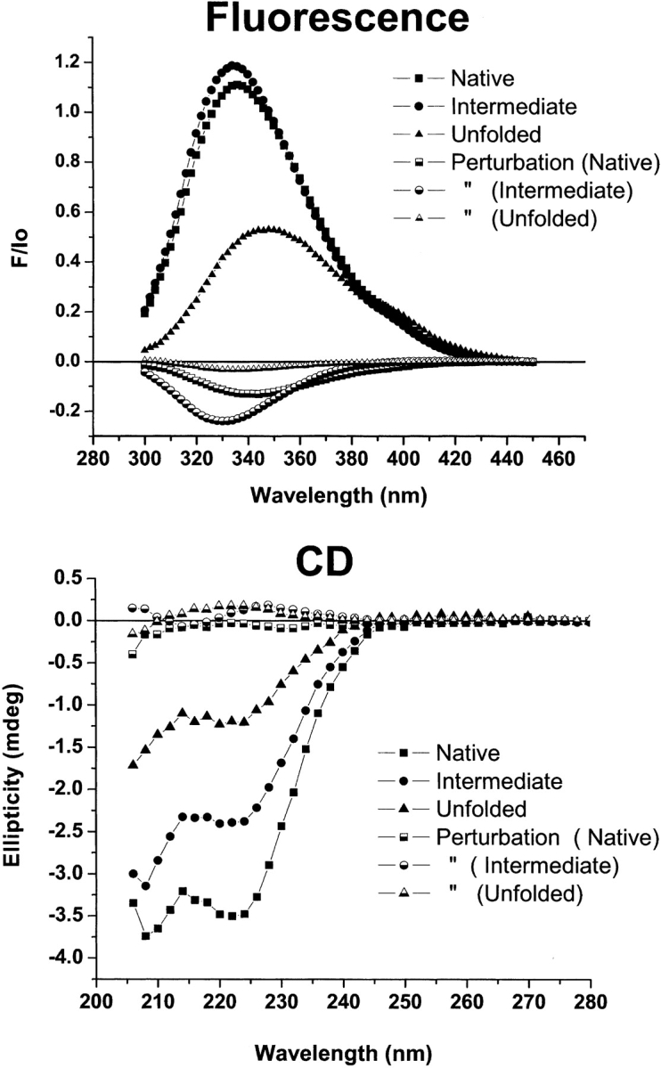
A recombinant form of an N-terminal fragment consisting of residues 4–220 of rhm CSF-β was subjected to denaturation by urea under conditions that preserve the native disulfides. Fluorescence and CD spectra from this titration are shown in Figure 1, A and B ▶. Relative fluorescence intensities at 340 nm and CD ellipticities at 222 nm are shown in Figure 2 ▶, A and B, respectively. Sharp transitions in the shapes and magnitudes of both sets of spectra are observed between 7.2 M and 8.4 M urea. From CD spectra of native rhm CSF-β, an α-helix content of 32% was estimated, in agreement with the X-ray crystal structure (Pandit et al. 1992). The spectrum of protein in the absence of urea has a double minimum between 208 nm and 225 nm, and changes very slightly in the pretransition phase below 6.2 M urea. Above 8.4 M urea, the CD spectra lack this shape and are smaller in magnitude than the native spectrum. They resemble CD spectra of other denatured proteins.

Figure 1.

rhm CSF-β titration spectra. rhm CSF-β (0.3 mg/mL) was titrated with urea, as described in Materials and Methods. Heavy lines are spectra collected at the urea concentrations shown in the legends. The thin solid lines are spectra identified as pretransition and posttransition spectra. Thin dotted lines are spectra measured over the structural transition. (A) Fluorescence spectra. (B) CD spectra.

Figure 2.

rhm CSF-β titration spectra at single wavelengths. Intensities of spectra at single wavelengths were selected for plotting (open circles). Points in the pre- and posttransition zones, marked with asterisks and diamonds, respectively, were fitted with linear and second order polynomials. Relative improvements in fitting were gauged with one-sided P-values for the F-statistic (see Results). (A) Relative fluorescence intensities at 340 nm. Pretransition F-test: P_F = 0.39 for quadratic vs. linear fits. Posttransition F-tests: insufficient data, fit to constant shown. (B) CD ellipticities at 222 nm. Pretransition F-test: P_F = 0.14 for quadratic vs. linear fits. Posttransition P_F = 0.44 for linear vs. constant fit.

The fluorescence emission spectra shown here were collected using an excitation wavelength of 280 nm. At urea concentrations below 7.5 M, the spectra are bimodal (Fig. 1A ▶). The shoulder at 305 nm is not present in the emission spectrum of native protein upon excitation at 290 nm. Tyrosine residues, which absorb weakly compared with tryptophan at 290 nm, are plentiful in rhm CSF-β. Therefore, the 305-nm shoulder is assigned to the fluorescence of tyrosine residues. Between 0 M and 7 M urea, the intensities of the peak and shoulder regions increase significantly, and there is a slight shift of the centroids of the spectra towards longer wavelengths as judged by their intensity-weighted mean wavelengths (from 353 to 354 nm). Between 7.5 M and 8.4 M urea, the peak intensity increases monotonically with urea concentration. At 8.4 M urea and above, the 305-nm shoulder is no longer visible. Note that this change in the relative contributions of tryptophan and tyrosine residues to the overall spectra cannot be observed at a single wavelength (e.g., 340 nm, Fig. 2A ▶). Between a urea concentration of 8.4 M and the end of the titration at 9.2 M, CD and fluorescence spectra do not change significantly at any wavelength. Together, these data imply that macrophage colony-stimulating factor (MCSF) unfolds in urea solutions via a single equilibrium between the native and unfolded states.

As noted above, reports of other two-state unfolding transitions generally attribute linear dependencies to the pre-and posttransition phases of denaturant. To construct a model of denaturant titrations that includes the direct effects of denaturant, it is necessary to have at least an approximate functional form for the dependence of this perturbation on the concentration of denaturant. To test whether the dependence of pretransition and posttransition spectra of rhm CSF-β on urea concentration is linear or not, fluorescence and CD spectra from these regions of the titrations were fit to first-degree and second-degree polynomials. Stars and diamonds in Figure 2, A and B ▶, indicate the pretransition and posttransition points selected for fitting. The residuals of these fits were compared using an F-test (Bevington 1969). In all cases, the improvement in fit from linear to quadratic was significant at less than the 90% level. Therefore, linear functions are considered adequate models for the urea concentration dependence of the perturbation spectra of rhm CSF-β.

Retinoid X receptor, a three-state unfolder

The second system examined is the denaturation by guanidine hydrochloride of the ligand-binding domain of human recombinant retinoid X receptor-α (RXRα), which binds 9-cis-retinoic acid and homologs. The protein exists as a homodimer in solution (Egea et al. 2001), and the X-ray crystal structure (Bourguet et al. 1995) indicates that it has an α-helical content of 66%. The CD spectrum of native dimer (Fig. 3A ▶) displays twin minima at 222 nm and 208 nm. Three phases of guanidine-induced RXRα unfolding are evident in Figure 3A ▶: a pretransition phase (native structure) below 0.8 M guanidine, a transition followed by a nearly unchanging phase from 2 M to 2.65 M, and another transition followed by the posttransition phase representing the unfolded structure above 4.1 M guanidine. The intermediate spectra are missing the minimum at 222 nm and intersect the unfolded spectra at ~205 nm, consistent with a transition to a distinct, mixed α-helical-unfolded secondary structure in the presence of 2.5 M guanidine. The three-phase structure of RXRα unfolding is not as evident when observed with fluorescence spectra (Fig. 3B ▶). The first pre-transition phase results in a blue-shifted spectrum (0.9 M guanidine). Above 1 M guanidine, all spectra lose intensity and become increasingly red-shifted as the protein unfolds. A clear posttransition phase occurring between 4.1 M and 5 M guanidine displays spectra that are sharply red-shifted compared to the native and intervening spectra, and therefore are assigned to unfolded protein, in agreement with the CD results. However, it would not be possible to detect and demarcate intermediate phases in the unfolding of RXRα, were it not for the CD titration. As reference points, the fluorescence spectra that demarcate the intermediate phases of unfolding according to CD are indicated in Figure 3B ▶.

Figure 3.

RXR titration spectra. RXRα (1.4 μM monomer) was titrated with guanidine HCl, and spectra were collected as described in Materials and Methods. Heavy lines are spectra collected at the concentrations shown in the legends. Thin solid lines are spectra identified as pretransition and posttransition spectra. In the case of fluorescence spectra between 2.10 M and 2.71 M guanidine, identification was made on the basis of the behavior of CD spectra in that range. Thin dotted lines and dashed-dotted lines are spectra measured over the structural transitions. (A) CD spectra. (B) Fluorescence spectra.

In Figure 4A ▶, fluorescence intensities at 340 nm are plotted against guanidine concentrations, and the pre- and post-transition points that were selected for fitting with polynomials are marked for comparison. Comparison of the residuals from fitting first-degree and second-degree polynomials to the pretransition points reveals that improvement of the fit through addition of one polynomial coefficient is not warranted at the 90% significance level. Similarly, there is no significant improvement to be gained from adding an extra parameter to a constant polynomial model of the unfolded state perturbation. Since, as shown in this plot, no intermediate state can be found, no model for its denaturant perturbation could be derived. Identical tests were applied to the ellipticities measured at 222 nm (Fig. 4B ▶). Here, CD spectra were collected at each of the guanidine concentrations shown, and the spectra (averages of intensities at 220–224 nm and standard error bars are shown in the figure) were subjected to the singular value analysis procedures described below to determine how many distinct spectra are needed to generate all the spectra in the data set. This analysis implies that native and unfolded spectra themselves are sufficient to account for the pretransition and posttransition spectra. Given that so few spectra could be collected over such short ranges in guanidine concentration, this is not surprising. The occurrence of titrations having narrow ranges of stability such as this is a major disadvantage to fitting denaturant titrations with graphical extrapolation methods.

Figure 4.

RXRα titration spectra at single wavelengths. (A) Fluorescence at 340 nm. Pretransition points and posttransition points are designated by plus signs and times signs, respectively. For other details, see Results. (B) CD ellipticities at 222 nm. Filled circles with error bars are results of SVD estimation of whole spectra at the indicated guanidine concentrations (see Results).

Although there appears to be an interruption in the curve in the range of 2–2.5 M in guanidine concentration, no attempt was made to choose between perturbation models based on so few points located near an intersection of two curves. Because the amplitudes of the perturbation spectra of tryptophan and tyrosine peptide analogs and the native and unfolded states in two-state and three-state titrations in urea and guanidine solutions are all adequately represented by linear functions of denaturant concentration, a linear model was chosen for the intermediate state of RXRα. How this model of the origin of the titration backgrounds is integrated with the fitting procedure is described in the Theory section.

Recovery of parameters and spectra from a simulation of three-state unfolding

In order to demonstrate the effectiveness of a method of data analysis, it is necessary to simulate one or more data sets using the model process that is presumed to generate that data, including sources of noise and error, and choices of adjustable parameters. Those parameters should then be recovered according to the method in question. In this study, amplitudes and locations of fluorescence and perturbation spectra of the pure states of RXRα were adjusted to produce titrations with clearly separated native, intermediate, and unfolded phases. A set of thermodynamic parameters were also chosen (Table 1), and the mole fractions of each state were calculated for 42 equally spaced concentrations of denaturant according to the linear models for the dependencies of free energy and perturbation on denaturant concentration, as described in the Theory and Materials and Methods sections. The mechanism chosen was that of a native dimer converting to a monomeric intermediate, followed by the complete unfolding of the intermediate. Noise was then added to the collection of spectra. In the laboratory, mixing protein and concentrated denaturant solutions is a source of significant systematic error. To simulate this error, random deviations in denaturant concentration were added to the model concentrations. These errors were distributed according to a normal function with a variance of 67% of the denaturant concentration interval. Experimental spectra contain random noise of two kinds: counting error, and dark current noise. The former was simulated with Gaussian random noise with standard deviation equal to 0.5% of the square root of the fluorescence intensity, and the latter with a standard deviation of 0.1% of the maximum fluorescence intensity. With these choices of error magnitudes, the resulting spectra resembled those collected from the guanidine denaturation of RXRα, that is, a “typical” data set. In order to estimate the sensitivity of the uncertainties in fitted parameter values to measurement noise, 32 datasets drawn from the same model parameters and random error distributions were generated. Each simulated titration was fit according to the procedure described in Analytical Procedures, assuming a six-dimensional basis set. The generalized hill-climbing global optimization procedure was employed with 100 initial points contained in the parameter intervals being searched for minimum error (0 ≤ ΔG°(0) ≤ 30 kCal/M and 0 ≤ c_m ≤ 12 M ). By searching this volume starting from a large number of initial points, this algorithm avoids entrapment in local minima. If multiple minima are present, a search from a large number of initial points will detect them. The 100 solutions from each simulation were sorted according to their median residuals, and the 60 values with the smallest residuals were retained. Table 1 lists the medians of the retained solutions together with the parameter values used to generate those data. Standard errors calculated from the fits are less than 10% of the corresponding parameter values, except for the free-energy change of the second equilibrium. In all cases, agreement between the simulation values and recovered values was well within one standard error. Figure 5 ▶ compares the component spectra recovered from the data analysis with those used to generate the data. Note the different scales in the two graphs. Errors in recovering species spectra are less than 1% of the simulated spectra. The recovered perturbation spectra are systematically smaller than the originals; however, the errors are at most 0.5% of the corresponding species spectra. In Figure 6 ▶, fluorescence intensities at 340 nm from all simulations are compared with intensities calculated from the recovered median parameter estimates and component spectra (solid curve).

Table 1.

Simulated and recovered thermodynamic parameters

Parameter	Simulated	Median ± S.E.	Mean ± S.E.
N2 ⇌ 2I
ΔG0(0)	14.0	13.7 ± 1.0	14.2 ± 1.1
CM	4.2	4.3 ± 0.3	4.2 ± 0.4
2I ⇌ 2U
ΔG0(0)	11.0	11.6 ± 4.4	14.0 ± 4.9
CM	4.0	4.0 ± 0.1	4.0 ± 0.1

Thirty-two simulated fluorescence data sets with random errors added were analyzed according to procedures outlined in Materials and Methods. Medians and means of estimates of thermodynamic parameters recovered by analyzing the 32 data sets are listed together with the parameters with which the data were simulated. Units for ΔG⁰ (0) are in units of kCal mole^−1; C_M is in units of molar concentration.

Figure 5.

Comparison of simulated and recovered three-state fluorescence spectra. The three species spectra and three perturbation spectra used to simulate a three-state titration are shown with line plots. A three-state model was fit to 32 simulated data sets with random noise as described in Results. The median parameter estimates were used to calculate expected spectra, shown as symbols. (A) Species spectra. (B) Perturbation spectra.

Figure 6.

Simulated and recovered fluorescence intensities at 340 nm. Fluorescence intensities from simulated data are plotted vs. denaturant concentration (circles). Intensities were recovered from fitting a three-state model to 32 simulated data sets that differ by random noise. One of these is shown (solid line). Intensities recovered from fitting a two-state model are shown as a dashed curve.

Determining the number of unfolding states with singular value analysis

In the analysis of the simulated data, the number of protein states was given a priori, so the determination of this number from the data itself was not needed. A method for deriving this number from experimental results will now be described.

The spectra of an equilibrium titration among n species will be combinations of as many as 2n component spectra. In practice, experimental spectra are sampled at a discrete set of wavelengths, representing the spectra as vectors (ordered lists) of intensities. If these 2n vectors are not linear combinations of each other, they form a basis set for all the spectra collected in the titration, and it follows from the fundamentals of linear algebra (Hoffman and Kunze 1971) that any other basis for this space must also contain 2n vectors. The first 2n columns in the U and V matrices of the SVD of the data matrix are such a basis.

Because noise is a component of experimental data, no singular values in the SVD of its data matrix are null. Instead, the relative information content of the columns in the U and V matrices in the SVD expansion is indicated by singular values that asymptotically approach zero along the diagonal of the S matrix. In parallel with the singular values, the first few columns of the U and V matrices contain most of the information in the experimental spectra. These are also the smoothest abstract spectra and titration curves in the set, as the SVD procedure concentrates random (uncorrelated) noise in the latter abstract basis spectra and titration curves. The task of distinguishing signal from noise, and the ambiguity thereof, lies mainly in the identification of the threshold between the significant singular values, that is, those signifying signals, and those representing noise.

Figure 7A ▶ is a semilogarithmic plot of the singular values derived from one of the simulated datasets discussed above. The fifth and higher singular values denote the noise-dominated components of the SVD of these data. The first three values are unambiguously greater in magnitude. The fourth singular value is greater than the fifth by only 0.01, or 0.1% of the maximum singular value. To decide whether the fourth set of components of SVD represent signal content in the data, we used SVD to fit the abstract basis spectra in U to the observed spectra incrementally. Analogous to fitting polynomials of incrementally increasing degree to an arbitrary function, we fit to the data matrix one U-column at a time, measuring the sum-of-squares residuals of the fit at each degree of complexity and comparing the improvement of each fit to those that preceded it. Eventually, the residuals consist entirely of noise, and adding more dimensions merely creates a model that improves the fit to noise in the data. The F-test (Bevington 1969; Wackerly et al. 2002) compares the effect of the addition of one parameter (or basis vector, in this case) on the sum-of-squares residuals and the number of degrees-of-freedom of the fit. The F-test returns the probability (as a one-sided P-value) that the residuals of the fit obtained with n basis vectors and those obtained with n-1 basis vectors are drawn from the same distribution. A high P-value implies that there has been no improvement in fitting the correct signal underlying the noise. Because SVD sorts singular values in decreasing order, P-values will become less sensitive to increases in model complexity once the boundary between signal-fitting and noise-fitting has been passed. P-values (P_F) for the fits to the matrix of simulated data are also shown in Figure 7A ▶. The P_F for a fit with four s-values is 0.039. There is a break in the curve at five s-values, where P_F = 0.108. With a larger basis, P_F increases more slowly and levels out at ~0.16. Using the foregoing principles, we conclude that P_F = 0.1 is the natural threshold between significant and insignificant s-values sought for the simulated data. Beyond this point, improvements in representing spectra cannot be distinguished from better fits to noise, and we conclude that a four-dimensional model is needed to reconstruct spectra of the titration, but that more complex models are not justified by these analyses.

Figure 7.

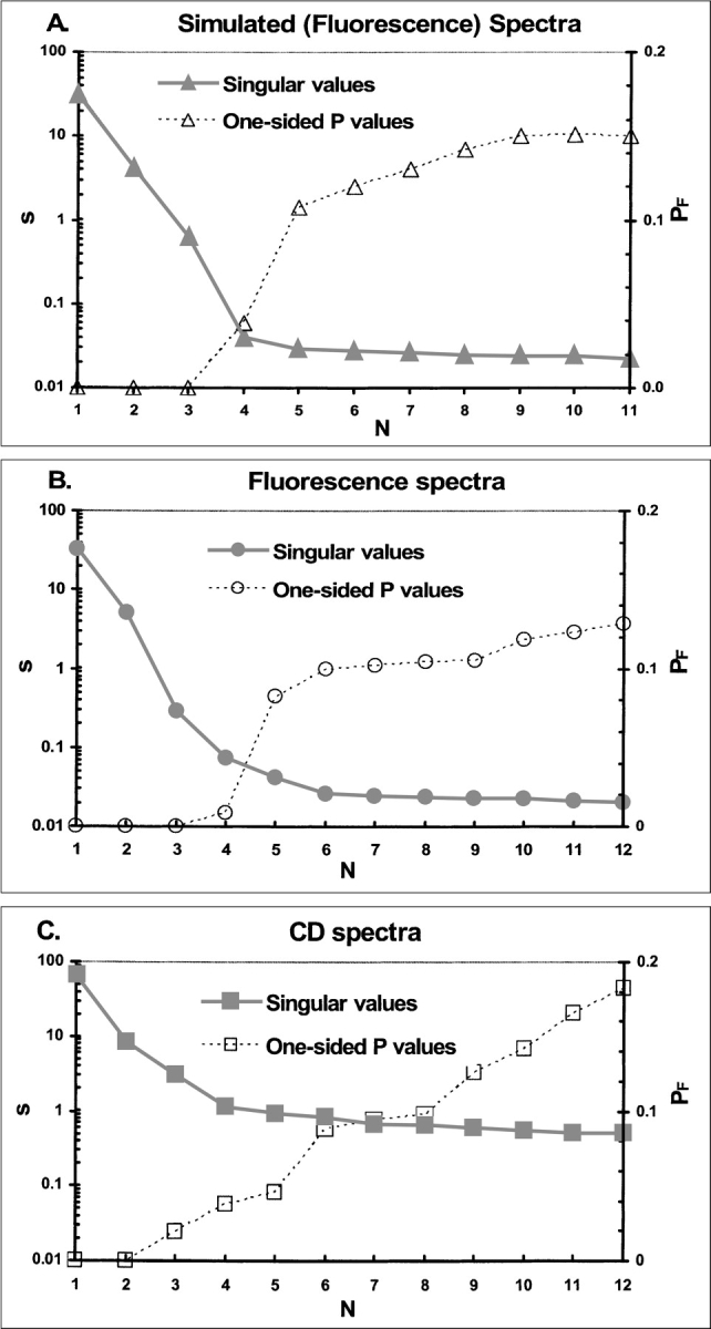
Singular value analysis of simulated and RXRα data. Logarithms of singular values from SVD of data matrices (solid symbols, solid lines) are plotted vs. their rank order (N) within the SVD. Open symbols with dashed lines represent one-sided P-values (P_F) for the F-statistic that compares a rank N approximation of the data matrix with the rank N-1 approximation. (A) Simulated fluorescence data. (B) Fluorescence spectra from the RXRα denaturation. (C) CD spectra from the RXRα denaturation.

A similar analysis of the s-values and F-test results of the fluorescence and CD observations of the titrations of RXRα with guanidine HCl was also performed. Figure 7, B and C ▶, shows the relationships of s-values and P_F levels to the number of dimensions in SVD reconstructions of the data matrices from these titrations. The transitions from large but decreasing s-values to small and approximately constant values are more gradual than for the simulated data. Again, breaks in the P_F curves occur around P_F = 0.1, where N = 6. In the case of these titrations, analysis of s- and P_F-values justify a five-dimensional SVD reconstruction of the data.

The simulated data were created with a six-dimensional model, yet only four dimensions were indicated by the singular value analysis (Fig. 7A ▶). There are two related explanations for this discrepancy. First, some protein component spectra, most likely perturbation spectra, may be too small, compared with experimental noise, to be detected by a singular value analysis. This would certainly be the case when the perturbation effect on the spectrum of one of the protein states is very small. Second, one or more component spectra may be nearly linearly dependent on the other component spectra. In that case, a basis vector in the SVD expansion of the experimental data matrix could be weighted by an s-value sufficiently small that it would be lost in the SVD representation of experimental noise. Nevertheless, underestimating the number of SVD components required to span the dataset will result in a faulty estimation of the thermodynamic and spectral parameters. When the simulated dataset was analyzed with a two-state model, and the calculated fluorescence intensities at 340 nm were compared with observed intensities, there were obvious trends in the errors, as shown in Figure 6 ▶ (dashed curve). The statistical significance of trends in the residuals generated by fitting two-state and three-state models to the reduced simulated data were quantified with runs tests (Wackerly et al. 2002), which determined that, while any runs in residuals of the three-state are random, runs in the two-state fit are systematic (data not shown).

When the RXRα experimental unfolding data were subjected to singular value analysis, the data appeared to be spanned by a five-dimensional basis, and a two-state model would only be four-dimensional. When a two-state model was fit to these data, the recovered fluorescence spectrum for the native species was negative over a range of wavelengths (Fig. 8A ▶), a clear impossibility. CD ellipticities at 222 nm that were calculated from the results of fitting two-state and three-state models are compared with observed ellipticities in Figure 8B ▶. The systematic errors in the two-state fit were confirmed with runs tests. Thus, the two-state model could be rejected on the basis of three criteria—the number of significant singular values, the presence of systematic errors in the fit, and the unreasonable fluorescence spectra of the calculated pure species.

Figure 8.

Comparing two-state and three-state fits to RXRα titration data. (A) Fluorescence spectra recovered from fitting a two-state model. (B) Circles are CD ellipticities measured at 222 nm (from Fig. 4B ▶). Ellipticities were reconstructed using median estimates of the thermodynamic parameters (see Table 2) and transformed data (S • V^T) for a three-state model (solid curve). The dashed curve shows ellipticities reconstructed from fitting a two-state model.

Results of fitting the unfolding titration of RXRα with a three-state model

The thermodynamic parameters recovered from fitting a three-state model to the CD and fluorescence titrations of RXRα are shown in Table 2 together with the results of a joint analysis of both datasets. The same procedure employed for the analysis of the simulated data (including parameter search by global optimization) was used to derive an estimate of thermodynamic parameters and to calculate residuals. In order to obtain confidence intervals for the parameter estimates, a collection of data drawn from the same distribution of residuals as the original was generated and analyzed as follows: Thirty-two new sets of residuals were simulated by resampling the residuals of the original set, and these were added to the calculated spectra to create 32 sets of bootstrapped data (Press et al. 1992). These were fit as before, and medians of the 32 sets of parameters, their standard errors, and matrices of correlation between the parameters were computed. Note that the standard errors of results of the joint analysis are an order of magnitude smaller than the standard errors of the individual fits (Table 2). This increase in precision is what one would expect from adding two error surfaces that possess elongated minima that intersect over a smaller and more isotropic volume of parameter space. This interpretation is confirmed by comparing the correlation matrices of the individual and joint analyses (Table 3). With the exception of the correlation between the midpoint concentration and the free-energy change of the first equilibrium, none of the correlations among the parameters derived from the joint analysis are strong, and most are roughly half the magnitude of the correlations among parameters derived from analyses of the individual datasets.

Table 2.

Recovered values of the thermodynamic parameters from bootstrapped unfolding titrations of RXRα

	Fluorescence	Circular dichroism	Joint analysis
N2 ⇌ 2I
ΔG0(0)	14.3 ± 0.1	11.2 ± 0.2	13.10 ± 0.05
CM	4.7 ± 0.1	5.4 ± 0.1	3.75 ± 0.02
2I ⇌ 2U
ΔG0(0)	13.2 ± 0.2	9.2 ± 0.3	11.77 ± 0.07
CM	3.1 ± 0.0	3.5 ± 0.1	3.55 ± 0.00

Units are the same as those in Table 1. Thirty-two hypothetical data sets were created by adding randomly permuted selections of the residuals from the initial fit to data calculated from the fit. These were reanalyzed using the same procedure. Results shown are medians of the 32 resampled data sets and their standard errors. The first two columns list the results from fitting fluorescence spectra and CD spectra individually. The third column lists results from joint fitting of both data sets.

Table 3.

Correlation coefficients between thermodynamic parameters

	Fluorescence					Circular dichroism					Joint analysis
N2 ⇌ 2I	ΔG0(0)	1				ΔG0(0)	1				ΔG0(0)	1
	CM	0.63	1			CM	0.68	1			CM	−0.96	1
2I ⇌ 2U	ΔG0(0)	−0.28	0.94	1		ΔG0(0)	0.69	0.94	1		ΔG0(0)	0.39	−0.4	1
	CM	−0.86	−0.92	0.38	1	CM	0.89	0.92	0.93	1	CM	0.31	−0.42	−0.05	1

Matrices of correlation coefficients were computed using the parameter estimates saved from fitting bootstrap-resampled data. Correlation matrices are symmetric; only the subdiagonal matrices are shown. Parameter designations are the same as in Table 2.

Figure 9 ▶ shows the species and perturbation spectra recovered from the analysis of RXRα data. Note that the fluorescence spectrum of the intermediate species is slightly more intense at its maximum than the native spectrum, and is slightly blue-shifted. The close resemblance of these two spectra and the magnitude of the perturbation spectrum of this species accounts for the apparent absence of a distinct intermediate state in the fluorescence titration of RXRα (Figs. 3A ▶, 4A ▶). The spectrum of the unfolded species is distinctly less intense and red-shifted compared to the other two spectra. The CD spectra of the three species are more distinct than the fluorescence spectra. The experimental spectra and the species spectra follow the same trend—from a native spectrum with evident α-helical character to a characteristic denatured state spectrum via an intermediate form. The perturbation spectra are very weak, as expected from the near-zero slopes of the pre- and posttransition ellipticities at 222 nm (Fig. 4B ▶).

Figure 9.

Species and perturbation spectra from fitting RXRα with the three-state model. Species and perturbation spectra from fitting RXRα titrations were reconstructed using median estimates of the thermodynamic parameters (Table 2) and transformed data. Filled symbols are species spectra. Half-filled symbols are corresponding perturbation spectra. (Top) Fluorescence spectra. (Bottom) CD spectra.

Discussion

To be useful, a method for the analysis of experimental data must enable the experimentalist to accurately estimate the values of parameters that quantify important physical characteristics of the system under study. To accomplish this, the analytical procedure must separate the signals that carry pertinent information about the system from extraneous elements that distort or obscure the signal. In the case of spectroscopic observations of protein unfolding equilibria, counting error, photo-detector noise, and mixing error make random contributions to the observed spectra. The random noise in these measurements is uncorrelated within and among the spectra of a titration. In the method described herein, the influence of random noise and error on the analysis is minimized by fitting to the weighted columns of the V matrix of the SVD of the data. The weights are the singular values given by the S matrix, which SVD sorts in decreasing order. Thus, the first few columns of the transformed data matrix have the greatest magnitude and will, therefore, dominate the fitting process. Random noise is pushed back into the many smaller components of the transformed data, in effect filtering the most important determinants of the fitting results.

In the ordered set of singular values, SVD also provides perhaps the most important resource for estimating the dimensionality of the model description of the equilibrium system. With noise-free data, this task is trivial—the number of nonzero singular values will equal the number of independent signals (spectra and titration curves) that generate the data set. In the presence of noise, all singular values will be nonzero and any choice of demarcation between signal and noise is approximate. The first few singular values are sufficiently above the magnitudes of the trailing values that they can be enumerated by inspection. A finer discrimination is provided by an analysis of the series of residual vectors resulting from incremental approximation of the data matrix with SVD bases. The procedure is identical to choosing a degree of orthogonal polynomial or the number of Fourier components to use when approximating noisy data. With each addition of component, the statistical significance of the loss of residual magnitudes is determined. The use of the F-test for this purpose (see Results) provided more definite cutoffs for approximating data matrices than singular values alone. Unfortunately, F-test results indicated fewer components than expected for the three-state data we analyzed. Information from runs tests can confirm the significance of perceived systematic runs in residual vectors, and underfitting results in nonphysical fluorescence spectra. Therefore, we conclude that use of this hierarchical analysis has resulted in reasonable and, in the case of simulations, accurate model assignments.

The presence of denaturant in the solvent influences the structure of tryptophan and tyrosine fluorescence emission bands and CD ellipticity. We have shown that when unfolding titrations are observed as entire spectra, this perturbation takes the form of difference spectra that are characteristic of each species. Because the mechanism of this phenomenon is not understood, the relationship between the magnitude of a perturbation spectrum and denaturant concentration must be represented by an empirical function. This function was assumed to be a polynomial in denaturant concentration. The responses of intensities of fluorescence and CD spectra of NAWA, NAYA, and the pure native and unfolded states of rhm CSF-β and RXRα to denaturants were adequately described with linear functions of urea and guanidine concentrations. We also assume that the perturbation spectrum of the intermediate species of RXRα depends linearly on guanidine concentration.

Once an approximation to the data matrix is chosen on the basis of a singular value analysis, the separable linear-nonlinear regression is performed as described in the Theory, Materials and Methods, and Results sections. The results of this fit, especially the species and perturbation spectra, are then examined. If a data matrix is reconstructed with too few SVD components, information is lost and the recovered parameters and spectra will not be accurate. For this reason, we reject models if the fluorescence spectra for pure species are negative, if the perturbation spectra are too large (comparable in magnitude to species spectra or larger), or if the CD species spectra assume an atypical shape for a protein (e.g., unusually large positive peaks at wavelengths longer than 200 nm, with large negative troughs in the corresponding perturbation spectra that compensate for the aberrations during the fitting). The residuals of the fit are also inspected for systematic trends that indicate that a portion of the titration curve has not been accurately fit, as was the case with the two-state analysis of the data simulated with a three-state model. In the event of failure, a model with a different number of intermediates is chosen, and the fitting and evaluation process is repeated.

The chance that an incorrect result will be accepted is further reduced when identical titrations are carried out using multiple structural probes. In the case of our studies of rhm CSF-β and RXRα unfolding, CD and fluorescence were both employed as probes. Because the thermodynamics of unfolding are properties of the sample, recovered thermodynamic parameters should not depend on the modes of observation. Significant discrepancies in standard free-energy changes or midpoint concentrations would indicate an erroneous fit, probably from choosing a model of insufficient complexity.

Simultaneous analysis of multiple experiments with different probes can also reduce the dispersion in values of the thermodynamic parameters. This is especially true if the loci of the minima in the distinct error surfaces are orthogonal to each other, in which case the long trough-like minima caused by interparameter correlations will be rendered more symmetrical and less extensive (Beecham 1992). The joint analysis of CD and fluorescence observations of RXRα unfolding reduced the standard errors of most parameters compared to the separate analyses (Table 2).

No procedure for analyzing equilibrium titrations, including that described above, can distinguish between different mechanisms of unfolding. The mechanism we assumed in simulating and analyzing the three-state titrations described in this report is the on-path unfolding model in which dissociation of the dimer in the first step, followed by unfolding of the monomeric intermediate in the second step. An alternative pathway involving a dimeric intermediate followed by dissociation to unfolded monomers was also fit to the data from the RXRα unfolding titrations. The free-energy differences between native and fully unfolded protein are in agreement when the results of the two fits are compared. Other techniques such as stop-flow refolding and unfolding kinetics and thermal denaturation may also be useful in resolving mechanistic questions such as this. Results of these studies will be described in future publications.

The methods described in this report have been subjected to two critical tests. First, a titration of a three-state system was simulated using thermodynamic parameters and component fluorescence spectra similar to those yielded by the analysis of RXRα. Random noise and errors with components commonly encountered in spectroscopic observations of denaturant-induced protein unfolding were included in the data. As described in Results, the agreement between the parameters and spectra used to simulate the data and those estimated from the fit were excellent, demonstrating that data generated by the assumed model could be successfully analyzed according to these methods. Second, if the model used to develop the methods described herein is valid, then it should be possible to demonstrate that those methods yield reasonable results when real three-state systems are analyzed. This was done by obtaining reasonable spectra and thermodynamic parameters from analyzing RXRα unfolding as described above. The reasonableness of component spectra was discussed above. The overall free-energy change of unfolding of RXRα is compared with those of three other proteins with 190 residues or more in Table 4. Only glutathione S-transferase is a monomer; the others are homodimers. cAMP receptor also unfolds via a three-state mechanism. The free-energy change calculated for RXRα is in the middle of this range. The changes in free energy per unit denaturant concentration are also comparable to those of other proteins in this molecular weight range—between 1 and 5 kCal/mole•M for each transition.

Table 4.

Comparison of standard free energy changes of unfolding in the absence of denaturant

Protein	ΔG0 (0) (kCal/mole)	Residues	ΔG0 (0)/residue (kCal/residue)
RXRα	26.4	244	0.11
Human pituitary growth hormone	27.8	191	0.15
Porcine glutathione S-transferase	25.3	207	0.12
E. coli cAMP receptor	19.2	209	0.09

RXRα results are from this study. All others are cited in Neet and Timm (1994).

Although designed to fill the need for methods of analysis of three-state titrations, these global methods yield the same results as the graphical background-subtraction-and-linear-extrapolation method applied to the unfolding of rhm CSF-β. The latter method yielded 21.6 ± 0.89 kCal/mole for ΔG⁰(0) and −2.71 ± 0.11 kCal/mole M for the slope of free energy versus urea concentration. The corresponding values for fitting by nonlinear fitting to whole-spectra data were ΔG⁰(0) = 23.0 ± 2.8 kCal/mole, m = −2.96 ± 0.37 kCal/ mole M.

Global data fitting—treating spectra as data and combining experiments using different kinds of spectroscopy—is a well established procedure for analyzing titrations where it is not necessary to correct for the perturbation background. Correcting for the perturbation background prior to nonlinear regression for the remaining parameters in the single-wavelength case is standard procedure for two-state equilibria. This has also been accomplished for three-state equilibria, provided arbitrary assumptions are made about the slope of the background for the intermediate species. However, when pure native-state or unfolded-state spectra are only available over a short range of denaturant concentrations, accurate measurement of background slopes may not be possible, and the slope parameter for the perturbation must be derived as part of the regression for the other parameters. In the present case, perturbation spectra and species spectra are always determined concurrently. To our knowledge, the integration of all these features in one analytical procedure is unique to the method presented here.

The integration of all these goals—global fitting of multiwavelength spectra of different types with concomitant correction for denaturant perturbation—is made possible by the compact linear-algebraic formulation of the fitting problem as described in the Theory and Materials and Methods sections and by the use of a global optimization routine to minimize the error function over the parameter space without calculation of explicit derivatives. The most important features of the former are the elimination of any spectra from the fitting expression so that the fitting can be done entirely in the space spanned by the V-vectors, with concomitant savings in time and reduction of computational error, and the separable formulation of the model in which the matrix of coefficients of component spectra with respect to the U-vectors is postmultiplied by the matrix function of the nonlinear thermodynamic parameters. For every step that the global minimization routine takes in the space of the (nonlinear) thermodynamic parameters, the linear parameters that minimize the total fitting error are determined. In this manner, the solution is reached by iteration in the thermodynamic parameter space. Casting the problem in separable form is also convenient for fitting combined data sets, as the thermodynamic parameters are properties of the protein-denaturant system and must be shared among all those sets.

In summary, this report describes a novel method for analyzing the thermodynamics of three-state protein unfolding titrations. Rather than estimate baselines, the effects of denaturants on the spectra of the individual components are obtained directly from the data analysis as perturbation spectra. Using this approach in combination with single value decomposition methods and a global analysis of data sets obtained by different spectroscopic techniques, the methodology was successfully applied to simulated data and experimental two- and three-state unfolding systems. This procedure should allow more precise estimation of thermodynamic parameters of three-state unfolding systems without unwarranted assumptions regarding baseline behaviors.

Theory

In a titration experiment, one measures changes in the concentrations of species at equilibrium as a function of the concentration of some titrant on which the free-energy changes of the component equilibria depend. The object of analyzing protein denaturation titrations is to estimate the values of parameters that characterize the relationship between experimental observations and thermodynamic properties of the system, according to some model of the denaturation process. The discussion that follows describes the most common thermodynamic model of protein denaturation, its transformation into a form amenable to solution of the problem, and the regression algorithm used to obtain the adjustable parameters of the model.

According to the most commonly used model for the stability of proteins in the presence of denaturants (Schellman 1978), the standard free-energy change of unfolding is a linear function of two parameters: the free energy change in the absence of denaturant [(ΔG⁰(0)] and a constant derivative of the free-energy change as a function of denaturant concentration. An alternate form of the same relationship, in which the concentration dependence is replaced by a unitless term, is better suited to fitting these experimental data:

(1)

In equation 1, c_m is the concentration of denaturant at which ΔG⁰(c), the standard free-energy change as a function of denaturant concentration, is zero. In the case of multistate equilibria, a separate ΔG⁰(0), c_m pair characterizes each transition.

The intensities of absorbance, fluorescence, and CD spectra of a pure chemical species are proportional to the concentration of the species and the molar signal for that species. As shown in Results, each species spectrum is accompanied by a perturbation spectrum whose magnitude is proportional to the concentration of denaturant. Thus, at each denaturant concentration, the measured spectrum contains contributions from n species at equilibrium, where species i contributes two spectra: φ_i, the spectrum per mole, and ψ_i, the corresponding perturbation spectrum per molar concentration of denaturant. The latter spectrum is additionally weighted with the denaturant concentration. If we let ^cj be the j-th concentration of denaturant, and let y_j be the total signal per mole of protein generated at the j-th denaturant concentration, then

where f_j,i is the mole fraction of species i at the j-th concentration of denaturant. This expression can be cast in block-matrix form as follows: Let Y be a matrix with y_j in column j, and let Φ and Ψ be matrices with species and perturbation spectra as columns. Then the model function for this system becomes

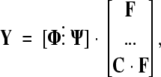(2)

where F = [f_i,j], the matrix of mole fractions, and C = [c_i,j], a diagonal matrix of denaturant concentrations.

For any choice of mole fractions and component spectra, the model function approximates the data matrix with a matrix of errors, E:

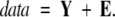(3)

Considerable simplification of the data fitting problem is achieved using the singular value decomposition (SVD) of the data matrix. The SVD is an eigenvector/eigenvalue expansion of the data matrix in terms of the product of three matrices: Matrix U consists of an orthonormal set of column vectors that span the space containing the measured spectra (the column space). Matrix S is the diagonal matrix of singular values arranged in order of descending magnitude, and V^T is the matrix whose rows span the row space of the data matrix (the titration curves at every wavelength). The singular values in S act as coefficients that weight the terms of the expansion. Substituting for data in equation 3 results in

(4)

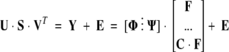
Equation 4 can be simplified by multiplying through by U^T. Define [P⋮Q] ≡

We now have

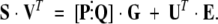(5)

Matrix [P⋮Q] contains the projections of the species and perturbation spectra on the row space of U^T. As such, it contains the coordinates of those spectra with respect to the column vectors in U^T. The error matrix is also dotted by U^T, so the product is the projection of the error matrix onto the row space of U^T (i.e., the column space of U). Because the columns of U are an orthonormal basis for the columns of E, U^T • E = Γ, where Γ is the matrix of coordinates of the errors in the space spanned by U. The left side of equation 5 is the projection of the data matrix onto the column space of U^T. Thus, equation 5 expresses the approximate relationship in “V-space” between the reduced data (S • V^T), the model function ([P⋮Q] • G), and the errors of the approximation. Note that no spectra appear in this expression, a desirable feature in that it minimizes computational work and the attendant numerical errors in the fit. In this form, the model is a separable linear/nonlinear function in which a linear term, [P⋮Q], multiplies the matrix of mole fractions, which are nonlinear functions of the thermodynamic parameters.

The nonlinear regression problem is to find the values of the thermodynamic parameters and the elements in [P⋮Q] that minimize the P-norm of the error term:

(6)

A separable linear/nonlinear least squares problem such as this can be solved by Variable Projection methods (Björck 1996) that take advantage of the interdependence of the linear and nonlinear parameters. Kaufman and others (Kaufman 1975) developed quadratically convergent variable projection methods for solving separable problems. Such methods rely on Gauss-Newton methods, which require calculations of Jacobian matrices. Because the 1-norm of the errors is a more robust estimator in the presence of data outliers than the 2-norm, the former was used to estimate the fitting errors. Because the 1-norm is not compatible with analytical derivative evaluations, a simpler, linearly convergent alternative to variable projection methods (Björck 1996) was used. According to this algorithm, once F and G have been calculated from trial values of the thermodynamic parameters, the matrix [P⋮Q] that minimizes the error norm for that fixed G can be found with linear least squares. The controlling optimization method calculates a step in the thermodynamic parameter vector, and the procedure is iterated until a convergence criterion is met.

Spectra of the pure species and the perturbations can be calculated by pre-multiplying the solution for matrix [P⋮Q] by U. However, this procedure retains all the noise present in the experimental spectra. The noise present in the reduced data matrix for two-state and three-state equilibria can be removed by deleting all rows beyond the first four or six rows, respectively. Fitting with filtered data may introduce bias into the adjustable parameters; but filtering noise from signals with SVD is an acceptable procedure (Branham Jr. 1990). In order to uncover underlying information masked by noise, the spectra reported here were filtered as follows: A filtered version of [P⋮Q] was estimated from the truncated version of S • V^T and the parameters estimated from the full data. Pre-multiplying the filtered [P⋮Q] by a matrix consisting of the first four or six columns of U yields the filtered species and perturbation spectra.

Materials and methods

Urea (Micro-select grade) was purchased from Fluka, and guanidine HCl (Ultrol grade) was purchased from Calbiochem. Trizma base, sodium EDTA, and potassium chloride were supplied by Sigma Chemicals. TCEP was purchased from Pierce, and CHAPS was purchased from Anatrace.

Fluorescence emission spectra were collected with an SLM-Aminco 8000 spectrofluorometer with a temperature-controlled sample turret. The excitation wavelength was 278 or 280 nm, and emission intensities were collected from 300 nm to either 460 nm or 500 nm at 1-nm intervals with an integration time of 1 sec per interval. All fluorescence intensities were collected as ratios of emitted counts to counts from a fraction of the excitation beam scattered from distilled water. Excitation and emission slit widths were both 8 nm. Spectra of urea or guanidine hydrochloride in buffer at intervals of 1 M denaturant were collected (10 replicate spectra per sample), and interpolated to all concentrations in the titration and smoothed in Mathematica. Following background subtraction, an additive baseline shift for each spectrum was measured and averaged at the largest five wavelengths, and subtracted to zero all spectra at those wavelengths.

CD spectra were acquired on a Jasco J-720 spectropolarimeter equipped with a Peltier device for controlling the temperature of the sample. Step scans were collected at 1 nm/step with an integration time of 1 or 2 sec. Generally, six replicate spectra were collected for each sample and averaged by the instrument. All scans began at 320 nm. Minimal wavelengths for the scans were determined by the point at which sample absorbance reached 1.5 OD, or at the wavelength at which the photomultiplier voltage exceeded 600 V. Spectra of urea in buffer at intervals of 1 M urea were collected (10 replicate spectra per sample), and interpolated to all concentrations in the titration and smoothed in Mathematica. Spectra were corrected for baseline shift as above, using wavelengths from 315 through 320 nm for calibration.

Rhm-CSF-β was a gift from Dr. Cynthia Cowgill (Chiron Corp., Emeryville, CA). Lyophilized protein was dissolved in Tris buffer (50 mM Tris HCl, 5 mM NaEDTA [pH 8.5]), and the buffer salts were diluted by ~3000× by repeated concentration and dilution in Tris buffer and concentrated to 30–40 mg/mL. In this form, the protein was stable for several days. Denaturation of the disulfide form of rhm-CSF-β was initiated by dilution to 0.3 mg/mL with Tris buffer with desired concentrations of urea. In all cases, protein was added slowly to a conical vial containing buffer/urea while stirring slowly with a spinvane. Mixing was stopped after 15 sec. Equilibrium was achieved after 2 h at room temperature. All spectra were acquired at 20°C. Denaturation under these conditions was fully reversible, as judged by recovery of native fluorescence and CD spectra upon refolding fully denatured protein.

The insert containing the RXRα E-domain was a gift from Pierre Chambon (Institut de Génétique et de Biologie Moleculaire et Cellulaire, Collège de France, Strasbourg, France). E. coli strain BL21(DE3 plys S) was transformed with a pet15B vector (Nova-gen) containing the insert. Cells were grown at 37°C to an OD of 0.6–0.7, chilled to 25°C, and induced for 4 h in the presence of 0.8 mM IPTG at 25°C. Cell pellets were sonicated on ice and centrifuged. Supernatant was equilibrated in bulk with Talon Co⁺⁺ resin in E/W buffer (50 mM KH₂PO₄ [pH 7.0], 0.3 M KCl), washed with E/W buffer containing 10 mM imidazole, poured into a column, and eluted with 150 mM imidazole in E/W buffer. To obtain a pure dimer species, the RXRα fractions were further purified by gel filtration on a Sephacryl S-200 or Superdex 200 column. Pooled fractions were concentrated and diluted into storage buffer (50 mM potassium phosphate, 0.5 M KCl, 1 mM TCEP, 0.5 mM CHAPS [pH 7.4]).

Protein in storage buffer was diluted to 1.4 μM in monomer concentration with various concentrations of guanidine HCl in storage buffer. Mixing was done as for rhm CSF-β. Samples were incubated at 30°C for 2 h, and spectra were acquired at the same temperature. Spectra of native protein were compared with spectra of protein that had been denatured and refolded, indicating that the unfolding was at least 95% reversible.

The mass action expressions describing the two three-state equilibria discussed in Results are the following:

(7)

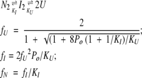(8)

The Mathematica global optimization package was from Loehle Enterprises (Naperville, IL).

Abbreviations

• CHAPS, 3-[(3-cholamidopropyl)-dimethylammonio]-1-propane sulfonate

• CD, circular dichroism

• RXRα, human retinoid-X-receptor-α ligand-binding domain

• NAWA, N-acetyl L-tryptophanamide

• NAYA, N-acetyl L-tyrosinamide

• P_F, one-sided P-value

• rhm CSF-β, recombinant human macrophage colony-stimulating factor β;

• SVD, singular value decomposition

• SSR, sum-of-squares residuals

• TCEP, Tris-2[carboxyethyl] phosphine

References

- Beecham, J.M. 1992. Global analysis of biochemical and biophysical data. Methods Enzymol. 21037–53. [DOI] [PubMed] [Google Scholar]
- Bevington, P. 1969. Data reduction and error analysis for the physical sciences. McGraw-Hill, New York.
- Björck, Å. 1996. Numerical methods for least squares problems, pp. 351–353. SIAM Press, Philadelphia.
- Bourguet, W., Ruff, M., Chambon, P., Gronemeyer, H., and Moras, D. 1995. Crystal structure of the ligand-binding domain of the human nuclear receptor RXR-α. Nature 375 377–382. [DOI] [PubMed] [Google Scholar]
- Branham Jr., R.L. 1990. Scientific data analysis. Springer-Verlag, New York.
- Callis, P. 1997. 1La and 1Lb transitions of tryptophan. Methods Enzymol. 278 113–122. [DOI] [PubMed] [Google Scholar]
- Egea, P.F., Rochel, N., Birck, C., Vachette, P., Timmins, P.A., and Moras, D. 2001. Effects of ligand binding on the association properties and conformation in solution of retinoic acid receptors RXR and RAR. J. Mol. Biol. 307 557–576. [DOI] [PubMed] [Google Scholar]
- Greenfield, N.J. 1996. Methods to estimate the conformation of proteins and polypeptides from circular dichroism data. Anal. Biochem. 235 1–10. [DOI] [PubMed] [Google Scholar]
- Harder, M.E., Leid, M.E., Deinzer, M.L., and Schimerlik, M.I. 2001. An improved method for analyzing multi-state unfolding titrations. Protein Sci. 10 (Suppl. 2): 180. [Google Scholar]
- Hoffman, K. and Kunze, R. 1971. Linear algebra. Prentice-Hall, Englewood Cliffs, NJ.
- Kaufman, L. 1975. Variable projection methods for solving separable nonlinear least squares problems. BIT 15 49–57. [Google Scholar]
- Johnson Jr., W.C. 1999. Analyzing protein circular dichroism spectra for accurate secondary structures. Proteins 35 307–312. [PubMed] [Google Scholar]
- Kuwajima, K. 1995. Circular dichroism. In rotein stability and folding, theory and practice, (ed. B. Shirley), pp. 115–135. Humana Press, Totowa, NJ.
- Lakowicz, J.R. 1999. rinciples of fluorescence spectroscopy, 2nd ed. Kluwer Academic/Plenum Publishers, New York.
- Neet, K.E. and Timm, D.E. 1994. Conformational stability of dimeric proteins: Quantitative studies by equilibrium denaturation. Protein Sci. 3 2167–2174. [DOI] [PMC free article] [PubMed] [Google Scholar]
- Noble, B. and Daniel, J.W. 1988. Applied linear algebra, 3rd ed. Prentice-Hall, Upper Saddle River, NJ.
- Pandit, J., Bohm, A., Jancarik, J., Halenbeck, R., Koths, K., and Kim, S. 1992. Three dimensional structure of dimeric human recombinant macrophage colony-stimulating factor. Science 258 1558– 1562. [DOI] [PubMed] [Google Scholar]
- Press, W.E., Teukolsky, S.A., Vetterling, W.T., and Flannery, B.P. 1992. Numerical recipes in Fortran 77, 2nd ed. Cambridge University Press, Cambridge, UK.
- Royer, C. 1995. Fluorescence spectroscopy. In rotein stability and folding, theory and practice (ed. B. Shirley), pp. 65–68. Humana Press, Totowa, NJ.
- Schellman, J.A. 1978. Solvent denaturation. Biopolymers 17 1305–1322. [DOI] [PubMed] [Google Scholar]
- Schmid, F.X. 1997. Optical spectroscopy to characterize protein conformation and conformational changes. In rotein structure: A practical approach (ed. T.E. Creighton ), pp. 261–296. IRL Press, Oxford, UK.
- van Holde, K.E., Johnson Jr., W.C., and Ho, P.S. 1998. rinciples of physical biochemistry. Prentice-Hall, Upper Saddle River, NJ.
- Wackerly, D.D., Mendenhall, W., and Scheaffer, R.L. 2002. Mathematical statistics with applications, 6th ed. Duxbury, Pacific Grove, CA.